Could short selling make financial markets tumble?

It is suggested to consider long term trends of financial markets as a growth phenomenon. The question that is asked is what conditions are needed for a long term sustainable growth or contraction in a financial market? The paper discuss the role of traditional market players of long only mutual funds versus hedge funds which take both short and long positions. It will be argued that financial markets since their very origin and only till very recently, have been in a state of “broken symmetry” which favored long term growth instead of contraction. The reason for this “broken symmetry” into a long term “bull phase” is the historical almost complete dominance by long only players in financial markets. Dangers connected to short trading are illustrated by the appearence of long term bearish trends seen in analytical results and by simulation results of an agent based market model. Recent short trade data of the Nasdaq Composite index show an increase in the short activity prior to or at the same time as dips in the market, and reveal an steadily increase in the short trading activity, reaching levels never seen before.

Stock markets are known to be notoriously difficult to predict. The impossibility of predicting has been formalized in the Efficient Market Hypothesis (EMH) which states that all available information is included in prices[1, 2]. Still without attempting specific prediction, it makes very well sense to ask which conditions are needed for a substainable trend, e.g. what is the “fuel” needed for a manifestation of a longer term bull or bear market? In this paper it is suggested to consider long term trends of financial markets as a growth phenomenon. The paper will discuss the role of traditional market players of long only mutual funds versus the recent arrival of hedge funds which take both short and long positions. Short selling[3, 4, 5] happens when speculators sell, say at time $t_{0}$ to price $P(t_{0})$, securities that they do not own but borrow. At a later time, say $t_{1}$, the speculator has to buy the security and give it back to it’s owner. In case of a price decline between $t_{0}$ and $t_{1}$ the speculator thereby makes the profit $P(t_{0})-P(t_{1})$. This is in contrast to long only funds who are only allowed to own securities and therefore can only profit when prices rise. To make an analogy with a physical system, it will be argued that financial markets since their very origin and only till very recently, have been in a state of “broken symmetry” which favored long term growth instead of contraction. The reason for this “broken symmetry” into a long term “bull phase” is the historical almost complete dominance by long only players in financial markets. Only with the recent arrival of investors that take up short positions is the symmetry slowly being restored, with the implications, as will be argued in this paper, of an increased probability for lasting decline of the markets, i.e. appearance of a long term “bear phase”.

Let us for a moment imagine a financial market could be completely determined by the action of just one powerful investor. This is in contrast to traditional economic theory which view the stock market as reflecting the state of economy, i.e. the prices of stocks should reflect present earnings as well as the expectation value of all future earnings of a given company. An alternative view would be to consider the stock market as the “motor” of the economy illustrated e.g. by the so called “wealth effect”, where increasing stock market prices leads to higher consumer confidence and spending, which in turns leads to larger earnings of companies making stocks rise, etc. ad infinitum. With this in mind, one could ask how big a fortune would such an investor need and which expectations about future developments in interest rate and dividends would ensure the investor to maintain a given growth of the market to his own profit? In order to answer these questions, consider first the case of a large mutual long-only fund that tries to control the market. The wealth of the fund, $W$, at any given time $t$ is:

$$W(t)=n(t)P(t)+C(t)~{},$$ (1)

where $P(t)$ is the price of the market, $n(t)$ is the number of market shares held and $C(t)$ the cash possessed by the fund at time $t$[6]. At each time step the dominating fund buys new market shares in order to push up the price of the market, creating an excess demand of market shares, $A(t)$. $A(t)$, give rise to the following equation for the return $r(t)$ of the market [7, 8]:

$$r(t)\equiv\ln(P(t+1))-\ln(P(t))=A(t)/\lambda,$$ (2)

where $P(t)$ is the price of the market and $\lambda$ is the liquidity of the market. The fact that the price goes in the direction of the sign of the order imbalance $A(t)$ is well-documented [9, 10, 11, 12, 13, 14]. $A(t)$ will first be taken a constant, $A(t)\equiv A$ i.e. we have

$$r(t)\approx{d\ln{P(t)}\over dt}=A/\lambda;\ \ P(t)=e^{At/\lambda},$$ (3)

and

$${dn(t)\over dt}=A;\ \ n(t)=At,$$ (4)

Besides expenses to keep on buying shares, the mutual fund get an income from dividends, $d(t)$, of the shares it’s already holding, and from interest rates, $r(t)$, of its cash supply $C(t)$. As will be seen the expectation of future dividends $d(t)$ and future interest rates $r(t)$ is crucial in designing a profitable strategy for the mutual fund. Since the aim of this paper is to study long term trends where changes in dividends can be much more important compared to changes in interest rates, $r(t)$ will be taken constant, $r(t)\equiv r$, and the focus will be the time dependence of $d(t)$. Consider first the simplest case where also $d$ is constant: $d(t)\equiv d$. The balance equation for the cash supply as a function of time therefore reads[15]:

$${dC(t)\over dt} = -{dn\over dt}P(t)+C(t)r+n(t)d+C_{\rm flow}(t,r(t),d(t),P(t),...)$$ (5)

$$= -Ae^{At/\lambda}+C(t)r+Atd+C_{\rm flow}(t,r(t),d(t),P(t),...)$$ (6)

The term $C_{\rm flow}(t,r(t),d(t),P(t),...)$ describes the possibility of additional inflow/outflow of money into the fund and as indicated can be thought of to depend on time, dividends, interest rates, the price of the market as well as many other factors like e.g. tax cuts etc[16]. In practice the inflow/outflow of liquidity often contributes a significant part to the total wealth of a mutual fund, but for clarity $C_{\rm flow}(t,r(t),d(t),P(t)...)$ will be taken equal to 0 first, before discussing the relevance of various functional forms below. It is preferable to express (6) in terms of the growth rate of the financial market, $\alpha\equiv A/\lambda$ and the cash in terms of the market liquidity, $\bar{C}\equiv C/\lambda$ in which case (6) become:

$${d\bar{C}(t)\over dt}=-\alpha e^{\alpha t}+\bar{C}(t)r+\alpha td$$ (7)

The solution of (7) reads:

$$\bar{C}(t)={\alpha e^{\alpha t}\over r-\alpha}-{\alpha dt\over r}-{\alpha d\over r^{2}}+{e^{rt}\over r-\alpha}\{-\alpha-{\alpha^{2}d\over r^{2}}+{\alpha d\over r}+C_{0}(r-\alpha)\}$$ (8)

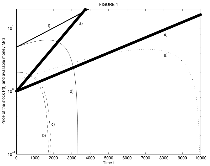
Figure 1: a) Price $P(t)$ of (3) as a function of time $t$ for $\alpha=0.2$. b) Cash $C(t)$ solution of (6) for the case $\alpha=0.2,r=0.1,C_{0}=2$ and $d=0.02$. c) Similar to curve b) but with $d=0.08$. d) similar to c) but with $C_{0}=5$. e) Price $P(t)$ of (3) for $\alpha=0.07$. f) Cash $C(t)$ solution of (6) for the case $\alpha=0.07,r=0.1,C_{0}=5$ and $d=0.02$. c) Similar f) but with $C_{0}=2$.

The condition to determine whether the mutual fund can impose a given growth of the stock market is that $C(t)>P(t)\ \ \forall t$ , i.e. the cash supply should always be large enough that yet another market share can be bought. The time dependence of (8) is dominated by the factors $e^{\alpha t}$ and $e^{rt}$ expressing the growth due to the stock market and interest rates respectively. For a stock market with a growth rate larger than the interest rate, $\alpha>r$ the first term on the r.h.s. of (8) dominates and becomes negative. In this case the growth of the stock market is not sustainable, and depending on the values of $r,d,C_{0}$ the investor will inevitably face a critical time, $t_{c}$, without enough money to secure further growth of the stock market. This situation is illustrated by the liquidity curve b) in Fig. 1 for the case $\alpha=0.2,r=0.1$ and $d=0.02$ [18]: after approximately 750 days the liquidity of the investor falls below the price of the stock market given by curve a) and he can no longer secure the 20% growth of the stock market. Had the investor received four times more in dividend, illustrated by curve c), $t_{c}$ would only be delayed by some few tens of days. Increasing the initial amount of liquidity, curve d), push $t_{c}$ further to the future, but eventually, for a “super” interest rate growth of the stock market, the investor will fall short of money and the growth have to stop. On the other hand for “sub” interest rate growth $\alpha<r$ the term $e^{rt}$ dominates and a sustainable growth depends on the values of $(\alpha,r,d)$. A $\alpha=7\%$ growth, curve e), with interest rates at $r=10\%$ and dividends $d=2\%$ can be sustained if the initial amount of money is large enough curve f) whereas lowering the initial liquidity the growth no longer becomes sustainable, curve g).

The Eq. (8) illustrates the case that the expectation of a constant dividend $d$ is not sufficient for a super interest rate market growth as e.g. was seen in the booming stock market growth of the ninetees. Clearly in that case the rise of the stock market was closely related to the sky rocketing expectations (justified or not) of future dividends. Using the Efficient Market Hypothesis an investor would expect the dividend to follow the growth of the stock market, and as will be seen super interest rate growth become possible in that case. If one take the dividend to increase proportional to the price $d(t)\equiv d_{0}P(t)$ (7) takes the form:

$${d\bar{C}(t)\over dt}=-\alpha e^{\alpha t}+\bar{C}(t)r+\alpha te^{\alpha t}d_{0}$$ (9)

with the solution:

$$\bar{C}(t)=\alpha e^{\alpha t}\{{td_{0}-1\over\alpha-r}-{d_{0}\over(\alpha-r)^{2}}\}+e^{rt}\{{-r\alpha+\alpha^{2}+\alpha d_{0}\over(\alpha-r)^{2}}+C_{0}\}$$ (10)

Curve b) in Fig. 2 illustrates a solution of (10) where a given amount of initial liquidity and a interest rate $r$ of 10%, a dividend $d_{0}$ of 2% is not enough to sustain a stock market growth of 20% (curve a)). On the other hand, for a higher initial dividend $d_{0}$ of 8% and same initial amount of liquidity, super interest growth of 20% does become sustainable (i.e. $C(t)\geq P(t)\ \ \forall t$) as illustrated by curve c). Sufficient initial funds are however required as illustrated by curve d) where a high initial dividend of 8% is not sufficient to avoid that the investor runs out of money ($C(t)<P(t)$ for $t\approx 2800$). For each set of values $(d_{0},C_{0})$ there exists a range of growth potentials, $\alpha$, for the investor $r<\alpha_{\rm low}<\alpha<\alpha_{\rm high}$. If the investor chooses to push up the market at a too slow growth rate $\alpha<\alpha_{\rm low}$ he eventually will run out of money at large time scales, whereas for a too fast growth $\alpha>\alpha_{\rm high}$ the investor will miss money to continue buying shares at short time scales. For the case illustrated by curve c) in Fig. 2, $\alpha_{\rm low}=0.18,\alpha_{\rm high}=0.32$.

The discussion so far has been on a large mutual long-only fund that tries to benefit from a constant growth in a stock market. Eqs.(6) and (9) also describe the more morbid situation where a hedge fund tries to benefit from a constant decline in a stock market by short selling. This situation is described in (9) taking $\alpha$ and $d_{0}$ negative. $d_{0}$ should be taken negative since a short seller has to pay dividend to the owner from which the stock was borrowed. Instead of the condition $C(t)>P(t)$ that was needed at all times for a mutual fund to keep on buying shares, a hedge fund would need to ensure that $W(t)>|n|P(t)$, i.e. the wealth of the hedge fund has to be sufficient that it can at any time buy back all the shares $n$ that it has borrowed (and sold) at an earlier time[19]. Figure 3 illustrates the case c) of Figure 2 with an interest rate of $r=10\%$ and dividend $d_{0}=8\%$ and the same initial liquidity $C_{0}=10$ but now $\alpha=-20\%$ (curve a). Since the wealth $W(t)$, curve c), is above $|n|P(t)$, curve b), it is indeed sustainable (and very profitable (!) as seen from the wealth curve) for a dominating hedge fund to force a continuous decline of the stock market. Notice that the case of a dominating long-only mutual fund that pushes the prices up versus the case of a dominating short-only hedge fund that makes the market tumble is only symmetric on short time scales. This is illustrated in curve d) in Fig. 3 which shows the wealth of a long-only fund with same parameters as the short-only fund curve c), except for the signs of $\alpha$ and $d$. Since the difference is however small on time scales relevant for trading (e.g. the difference in wealth is less than 2% after 5 years for the example given in Fig. 3) the difference will be ignored in the following.

One can think of many different and relevant expressions of the flow term $C_{\rm flow}(t,r(t),d(t),P(t),...)$. The simplest case where customers add/subtract a constant flow of money per time unit, $C_{\rm flow}(t,r(t),d(t),P(t),...)=\mu$, would not change anything of the analysis presented of (6) and (9) since $e^{\alpha t}$ and $e^{rt}$ would still be the dominant factors. Taking into account the interest rate in the inflow/outflow, $C_{\rm flow}(t,r(t),d(t),P(t),...)=\mu e^{rt}$, would create a dominant $\mu te^{rt}$ term in the case of a constant dividend (6). However in the more relevant case where the dividend follows the price, $d=d_{0}P(t)$ (9) super interest market growth would still be dominated by the ${td_{0}\over\alpha-r}\alpha e^{\alpha t}$ term and the conclusions presented above would remain unchanged.  

The eqs. (6) and (9) express the case of one single powerful investor that has enough liquidity to drive the market. This is clearly not a very realistic situation, but as will be seen it helps understanding the much more realistic and complex case of a group of investors that all try to drive the market for their own profit. One very much studied market model with competing agents is the so called “Minority Game” (MG) introduced by Challet and Zhang [20]. In the “Minority Game” the first approximation is to include only the direction of a market move by representing a financial time series as a binary time series $B(t)$ with 0 corresponding to a down move and 1 to an up move. Having in total $N$ agents, each agent $i$ possesses a memory of the last $m$ digits of $B(t)$. A strategy gives a prediction for the next outcome of $B(t)$ based on the history of the last $m$ digits of $B$. Since there are $2^{m}$ possible histories, the total number of strategies is given by $S=2^{2^{m}}$. Each agent holds the same number $s$ (in general different) of strategies among the $S$ possible strategies. At each time $t$, every agent uses her most successful strategy (in terms of payoff, see below) to decide whether to buy or sell an asset. The agent takes an action $a_{i}(t)=\pm 1$ where $1$ is interpreted as buying an asset and $-1$ as selling an asset. The excess demand, $A(t)$, at time $t$ is therefore given as $A(t)=\sum_{i=1}^{N}a_{i}(t)$. The return and the price of the market is as before given by (2) In the MG the payoff function of a strategy, $g^{\rm MG}_{i}(t)$, was rewarding strategies that a each time step belong to the minority decision: $g^{\rm MG}_{i}(t)=-a_{i}(t)A(t)$. However as stressed in another paper, ([21]), in real markets, the driving force underlying the competition between investors is not a struggle to be in the minority at each time step, but rather a fierce competition to gain money. Introducing profit as the selection mechanism for the strategies the payoff function was shown to take the form[21]: $g^{\$}_{i}(t+1)=a_{i}(t)A(t+1)$ The same payoff function was also used in another market model by Giardina and Bouchaud[22, 17]. Consequently the market model with this payoff function was called the $\$$-game as a reminder that profit drives the selection of strategies.

Figure 4 illustrates one price history (fat solid line) of the $\$$-game with $N=20$ agents, $r=10\%$, $d_{0}=8\%$ assuming like before that the dividend follows the market price $d(t)=d_{0}P(t)$. The parameter values used were $s=4,m=8,C_{0}=50$. Stochasticity was introduced via the initial strategies hold by the agents as well as by $N$ additional “noise” agents who at each time step made a random decision to either sell or buy one market share. The liquidity parameter, $\lambda$, in (2) was determined using the assumption that an univocal decision of all the agents to sell an asset should lead to a “crash” of 10%, i.e. from the condition $r(t)=-2N/\lambda=-10\%$. The 10% was chosen to mimic some of the very largest crashes seen in financial markets. Thin dotted lines represent the 5%, 50% and 95% quantiles (from bottom to top) respectively, i.e. at every time $t$ out of the 1000 different initial configurations only 50 got below the 5% quantile line, 500 got below the 50% quantile and 950 below the 95 % quantile. The average behavior of an agent can now be understood using the analysis of eq.’s (1)-(10)

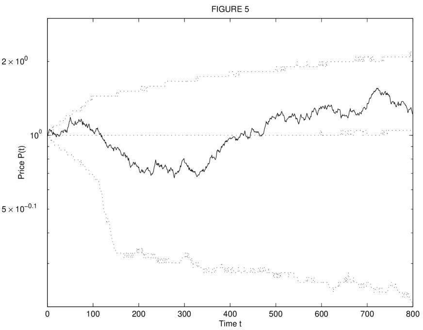
Figure 5: Same as figur 4 but with $\rho=0.2$

All the $N$ agents in figure 4 were long-only, i.e. they correspond to the case represented in figure 2 curve c). As predicted from the analysis of (9) the price $P(t)$ is in average tilted towards positive returns. Figure 5 represents simulations with the same parameter values as in figure 4 except that a fraction, $\rho=0.20$ of the agents can be both short and long. As can be seen from the 5% quantile, the introduction of agents that can take short positions clearly increases the probability significantly for a lasting bearish trend. Increasing $\rho$ to 0.4 amplifies this tendency, again in accordance with (9) as illustrated by the short-only hedge fund figure 3 curve c.  

Figure 7 shows the Nasdaq Composite index (fat solid line) as well as statistics of short selling over the time period 1/1 2000 - 1/8 2003. Dotted line represents the fraction of change in shares shorted, $n_{s}(t)$, defined as the monthly total number of change in shares shorted divided by the total monthly share volume[23]. The dashed line represents the cumulative fraction of change in shares shorted, $Q_{s}(t)=\sum_{t^{\prime}=0}^{t}n_{s}(t^{\prime})$. Both $n_{s}(t)$ and $Q_{s}(t)$ have been multiplied with a factor $10^{5}$ in order to make possible a comparison with the temporal evolution of the Nasdaq index. An interesting quantity in the present context would be the short activity, $A_{s}(t)$, simply defined as the total volume of short transactions divided by the total volume of transactions. Notice that $n_{s}(t)$ gives the lower bound on $A_{s}(t)$ since short positions opened and closed (or vice versa) within a month are not counted in $n_{s}(t)$ whereas they would be in $A_{s}(t)$. Since $n_{s}(t)$ typically varies between 0.1-0.6 % it is not unreasonable to assume $A_{s}(t)$ to be one order of magnitude larger, i.e. some few %. This means that the short activity on the Nasdaq index could be in the neighborhood that lead to a high probability of a lasting bearish trend seen in e.g. Fig. 4-6.

Simple visual inspection of the short trade data in Fig. 7 reveals an increase in the short activity $n_{s}(t)$ prior to or at the same time as dips in the market (see e.g. spring and fall 2000, summer 2001, fall 2002). Looking at the overall activity clearly confirms this pattern with a steadily increase in the cumulative short trading activity $Q_{s}(t)$ over the time period 2000 till summer 2001 and a steadily decrease of the market in the same time period. It is puzzling however, that one see an continuous increase of short activity so far in 2003 where the market also has made an increase. Either the market is right and short sellers will have to cover their positions in further progress of the market (i.e. $Q_{s}(t)$ should decrease in the future), or the short sellers got it right and the market is in for a future dip[24].  

It is clearly not easy to estimate precisely what impact short trading has on the evolution of financial markets. Still this paper has tried to point out some of the dangers connected to short trading as illustrated by the appearing of long term bearish trends seen in the analysis of (9) and by the simulation results in Fig. 4-6. It should be noted from Fig. 4-6 that even as the fraction of agents that use short trading increase, the probability for a long term “bullish” phase remain unchanged as illustrated by the 95% quantile lines which are unchanged in all three cases. This highlights that the danger with short selling is not when the markets are already in a long term bullish phase, since short sellers then are forced to cover their positions. The real danger is instead when a downwards spiral of the markets has begun, in which case an increase in short trading activity will only increase the downward trend. Looking at the bad performance of the markets over the past years together with the increase in short selling activity, which was virtually absent just few years ago, the present study suggest the possibility that financial markets could have entered a new era not seen so far.  

The author thanks D. Sornette for useful discussions.

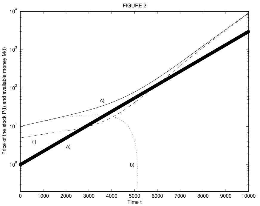
Figure 2: a) Price $P(t)$ of (3) as a function of time $t$ for $\alpha=0.2$. b) Cash $C(t)$ solution of (9) for the case $\alpha=0.2,r=0.1,C_{0}=10$ and $d=0.02$. c) Similar to curve b) but with $d=0.08$. d) similar to c) but with $C_{0}=5$.

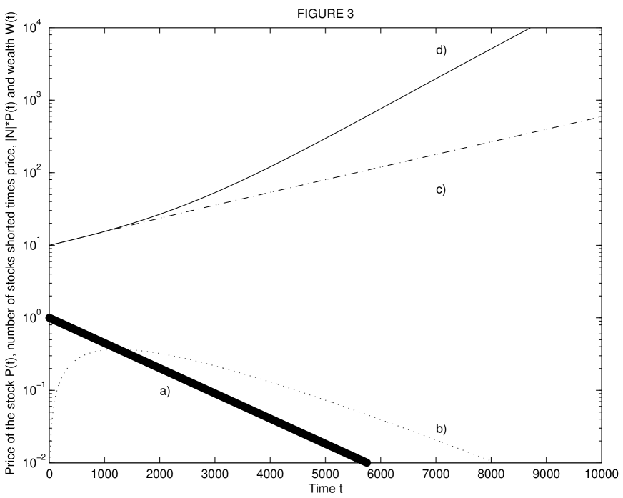
Figure 3: a) Price $P(t)$ of (3) as a function of time $t$ for $\alpha=-0.2$. b) $|n|P(t)$ for the case $\alpha=-0.2,r=0.1,C_{0}=10$ and $d=-0.08$. c) Wealth, $W(t)$ as a solution of (9) and (1) for the parameters of curve b). Same as curve b) except for signs of $\alpha,d$, $\alpha=0.2$ and $d=0.08$.

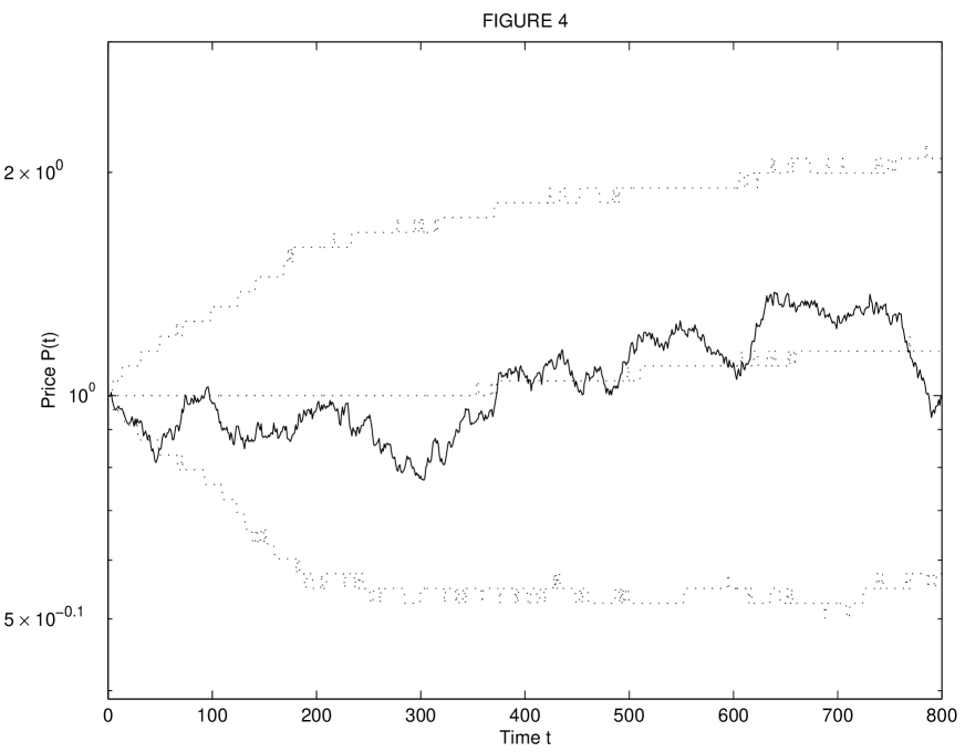
Figure 4: Fat solid line: price $P(t)$ from one configuration of the $\$$-game with $N=20$ agents, $r=10\%$, $d_{0}=8\%$ (assuming dividend $d(t)=d_{0}P(t)$). The parameter values used were $s=4,m=8,C_{0}=50$. Stochasticity was introduced via $N$ additional “noise” agents. The fraction of agents allowed to take short positions, $\rho=0$. Liquidity parameter $\lambda=0.0025$. Thin dotted lines represent the 5%, 50% and 95% quantiles (from bottom to top) respectively, i.e. at every time $t$ out of the 1000 different initial configurations only 50 got below the 5% quantile line and similarly for the other quantile lines.

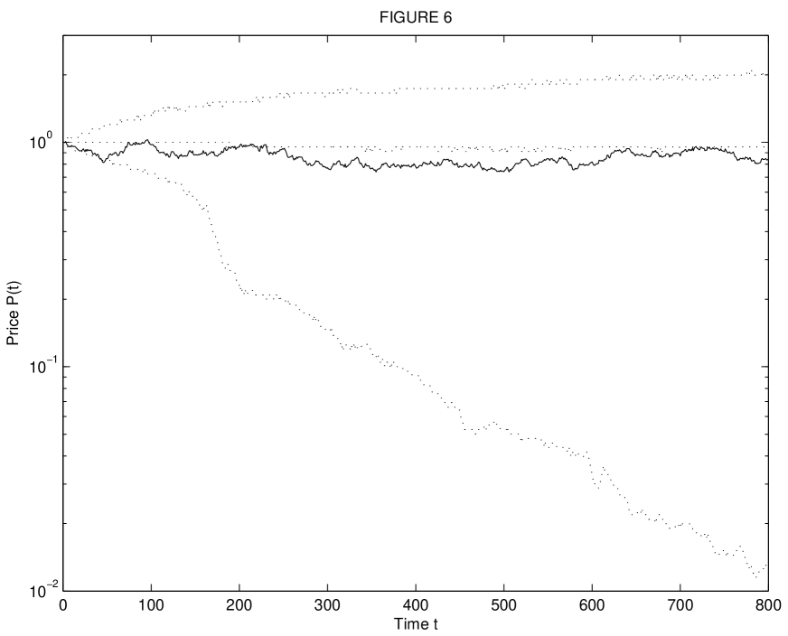
Figure 6: Same as figur 4 but with $\rho=0.4$

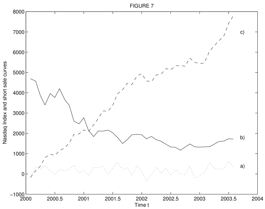
Figure 7: Fat solid line represents the Nasdaq Composite index. Dotted line represents the fraction of change in shares shorted, $n_{s}(t)$, defined as the monthly total number of change in shares shorted divided by the total monthly share volume. The dashed line represents the cumulative fraction of change in shares shorted, $Q_{s}(t)=\sum_{0}^{t}n_{s}(t)$. Both $n_{s}(t)$ and $Q_{s}(t)$ have been multiplied with a factor $10^{5}$.

References

- [1] E.F. Fama, Journal of Finance, 25, 383 (1970).
- [2] P. A. Samuelson, Industrial Management Review, 6, 41 (1965).
- [3] “Role of Speculative Short Sales in Price Formation: Case of the Weekend Effect”, H. Chen, V. Singal, preprint (2001);
- [4] “A Fuller Theory of Short Selling” H. D. Platt, preprint (2002).
- [5] “Bubbles in Experimental Asset Markets: Irrational Exuberance No More”,L. F. Ackert, N. Charupat, B. K. Church and R. Deaves, Federal Reserve Bank of Atlanta Working Paper (2002).
- [6] By a market share is understood a portfolio of stocks from which the financial market index is composed.
- [7] Bouchaud, J.-P. and R. Cont, Eur. Phys. J. B 6, 543 (1998).
- [8] Farmer, J.D., Int. J. Theo. Appl. Fin. 3, 425 (2000).
- [9] Holthausen, R.W., R.W. Leftwich and D. Mayers, J. Fin. Econ 19, 237 (1987).
- [10] Lakonishok, J. A. Shleifer, R. Thaler and R.W. Vishny, J. Fin. Econ. 32, 23 (1991).
- [11] Chan, L.K.C. and J. Lakonishok, J. Fin. Econ. 33, 173 (1995).
- [12] Maslov, S. and M. Mills, Physica A 299, 234 (2001).
- [13] Challet, D. and R. Stinchcombe, Physica A 300, 285 (2001).
- [14] V. Plerou, P. Gopikrishnan, X. Gabaix and H. E. Stanley, Phys. Rev. E 66, 027104 (2002).
- [15] A similar set of eq.’s [1-5] were used in [17] to explain bubble formation in an agent based model.
- [16] “Evidence of Fueling of the 2000 New Economy Bubble by Foreign Capital Inflow: Implications for the Future of the US Economy and its Stock Market”, D. Sornette and W.-X. Zhou, preprint, Cond.-Mat/0306496 (2003).
- [17] I. Giardina and J.-P. Bouchaud, Eur. Phys. J. B 31 421 (2003).
- [18] Typical values of will be used rather than trying to model a specific market and time period.
- [19] For simplicity the possibility of leverage is ignored.
- [20] For an introduction to the Minority Game see e.g. the papers: D. Challet and Y.-C. Zhang, Physica A 246, 407 (1997); ibid 256 514 (1998); R. Savit, R. Manuca and R. Riolo, Phys. Rev. Lett. 82, 2203 (1999); A. Cavagna, Phys. Rev. E 59 R3783, (1999). See also the special webpage on the Minority Game by D. Challet at For more specific applications of the Minority Game to financial markets see e.g. D. Challet et al., Quant. Fin 1, 168-176 (2001); M. Marsili, Physica A 299, 93, (2001); N. F. Johnson et al., Int. J. Theor. Appl. Fin. 3, 443 (2001); Johnson N. F. et al., Physica A 299, 222 (2001); Lamper, D., S. D. Howison and N. F. Johnson, Phys. Rev. Letts. 88, 017902, U190-U192.
- [21] J. Vitting Andersen and D. Sornette, Eur. Phys. J. B. 31 141 (2003);
- [22] I. Giardina, J.-P. Bouchaud, Physica A bf 299 28 (2001);
- [23] The short date can be retrieved directly without charge at the Nasdaq Composite home page:
- [24] Such a dip has actually been predicted to happen: D. Sornette and W.-X. Zhou, Quantitative Finance 2, 468 (2002); See also D. Sornette and W.-X. Zhou, “Predictability of Large Future Changes in Complex System”, preprint at cond-mat/034601, D. Sornette “Why Stock Markets Crash” (Critical Events in Complex Financial Systems) (Princeton University Press, Princeton, NJ 2003).