Theory of polyelectrolytes in solvents

Abstract

Using a continuum description, we account for fluctuations in the ionic solvent surrounding a Gaussian, charged chain and derive an effective short-ranged potential between the charges on the chain. This potential is repulsive at short separations and attractive at longer distances. The chemical potential can be derived from this potential. When the chemical potential is positive, it leads to a melt-like state. For a vanishingly low concentration of segments, this state exhibits scaling behavior for long chains. The Flory exponent characterizing the radius of gyration for long chains is calculated to be approximately $0.63$, close to the classical value obtained for second order phase transitions. For short chains, the radius of gyration varies linearly with $N$, the chain length, and is sensitive to the parameters in the interaction potential. The linear dependence on the chain length $N$ indicates a stiff behavior. The chemical potential associated with this interaction changes sign, when the screening length in the ionic solvent exceeds a critical value. This leads to condensation when the chemical potential is negative. In this state, it is shown using the mean-field approximation that spherical and toroidal condensed shapes can be obtained. The thickness of the toroidal polyelectrolyte is studied as a function of the parameters of the model, such as the ionic screening length. The predictions of this theory should be amenable to experimental verification.

I Introduction

A distinguishing feature of biopolymers is the presence of charges along the chain and their subsequent interaction with each other and ionic aqueous solvents. Yet another aspect is the semi-rigidity of some biopolymers. In this sense, biopolymers differentiate themselves from polymer melts, which are neutral, and most theoretical treatments involve the treatment of flexible polymers. Furthermore, these theoretical treatments of melts almost exclusively use models of a self-excluded volume nature. A general treatment of electrostatic interactions between charges on a polymer is crucial in order to extend the validity of theoretical models to bio-polymers, polymers exhibiting counter-ion condensation in ionic solvents, etc. frey_1 ; frey_2 ; frey_3 ; hinner .

This paper lays a field-theoretic foundation for a theoretical treatment of charged polymers in ionic solutions. Technically, the theory applies to flexible polyelectrolytes. However, we have argue that by choosing the Kuhn length to be the correlation length of a semi-rigid polymer, it should be possible to address the physics of semi-flexible polymers. The intent is not only to understand the behavior of the radius of gyration with chain length, but also to gain a basic knowledge of condensation phenomena. Our calculations of the radius of gyration generalize standard treatments for melts. A  mean-field approach was employed to develop a phase diagram for condensation/non-condensation of charged polymers. In this endeavor, we found the recent experimental paper by Butler et albutler very useful.

For the case of excluded volume interactions in polymer melts, it was shown by deGennesdeG1 and otherscloizeaux ; oono ; shirish0 that in the limit of low number concentration of monomers, the physics of polymers is analogous to the onset of a second order phase transition. It will be shown that a similar situation ensues when considering polyelectrolytes. The Flory exponent in this case, for long chains, is argued to be identical to the classical case. This is in distinction to the argumentsbarrat given by Katchalskykat and Floryflory-el for polyelectrolytes, where a long-range, unscreened Coulomb interaction was employed and the effects of any solvent were ignored.

This paper develops a model which begins with a screened Coulomb interaction between native electron charges and adsorbed counter-ions along the segments of a Gaussian chain. This screening length is independent of the solvent properties. These charges also interact with the surrounding ionic solvent, treated as a continuum. The theory in this paper continues the development of a functional integral techniqueshirish0 which begins with the formulation of a system of many homopolymeric flexible chains, and whose segments interact through a finite-range potential.

The functional integral technique utilized in this paper is different from the coarse-graining method employed by Fredrickson et al.fred Fredrickson et al use the number density of the polymer segments as the order parameter. The advantage afforded by this technique is that the interaction term becomes quadratic and hence trivial to calculate. However the entropy, or free-chain part of the energy functional becomes non-linear, complex and hence presents a computational challenge. The order parameter introduced in our paper is a probability amplitude whose absolute square corresponds to the number density of segments. The free-chain portion of the energy functional is linear in this approach, while the interaction term remains understandably non-linear and difficult computationally. The positive semi-definite form of our energy functional may also offer some computational advantages. Our formalism can be viewed as a generalization of the self-consistent field theory used by Curro’s group.deG1 ; curro The model of interaction used in this paper differs somewhat from that utilized by Curro et al. Our approach is most similar to that of Kleinertkleinert ; ferrari , but the scope of our study is broader.

Functional integration is used to integrate over the fluctuations in the ionic solvent, and derive an effective interaction between the charges on the chain. This interaction is repulsive at short distances, and attractive for larger separations. The chemical potential $\mu$ corresponding to this interaction can be computed. The chemical potential changes sign, depending on the parameter regime. Using the interpretation of $\mu$ as the energy required to add a segment (monomer) to the system, one associates $\mu>0$ with melt-like behavior, and $\mu<0$ with a condensed state. Indeed it will be shown that when $\mu<0$, it is possible for a single strand of polyelectrolyte to condense into a toroidal shape. Spherical shapes are also possible.

II The basic formalism

We reproduce here briefly for completeness, the functional integral formulation of a homopolymer chain. For the record, it must be stated that this formalism differs from the standard mapping of the self-avoiding walk of a single chain onto a $\phi^{4}$ field theory.deG1 ; cloizeaux It can be generalized in a straightforward way to deal with many chains. Technically speaking, the model is restricted to flexible chains. However, if one treats the segment length as a Kuhn length, i.e. as an effective distance which represents the correlation length of a semi-flexible polymer, then one expects this model to reproduce the overall features of a semi-rigid chain as well.

The probability distribution $G_{0}(1,2;n)$ for a single Gaussian chain may be represented bydoi-ed :

$$G_{0}(1,2;n) =\left({3\over 2\pi b^{2}|n|}\right)^{3/2}\exp\left(-{3\ |\vec{R}_{1}-\vec{R}_{2}|^{2}\over 2|n|b^{2}}\right)$$ (1)

$$\sim\int_{\vec{R}_{2}}^{\vec{R}_{1}}{\cal D}\vec{R}(n^{\prime})\exp-\left[\left({3\over 2b^{2}}\right)\int_{0}^{n}dn^{\prime}\left({\partial\vec{R}(n^{\prime})\over\partial n^{\prime}}^{2}\right)\right]$$

$$\equiv\langle 1,n|\left[\partial_{n^{\prime}}-\left({b^{2}\over 6}\right)\nabla^{2}\right]^{-1}|2,0\rangle$$

where $b$ is the Kuhn length of the polymer as discussed above, and where $\partial_{n^{\prime}}\equiv{\partial\over\partial n}$. This expression is obtained by considering only the entropy of a flexible chain.

$G_{0}(1,2;n)$ can also be thought of as the Green’s function for the diffusion operator in three dimensions, as indicated by the last of Eqns. 1.

Alternatively, one knows from methods in functional integration thatkaku :

$$\langle 1,n|\left[\partial_{n}-\left({b^{2}\over 6}\right)\nabla^{2}\right]^{-1}|2,0\rangle~{}\sim~{}\int{\cal D}^{2}\psi~{}\psi^{*}(\vec{R}_{1},n)\psi(\vec{R}_{2},0)\exp-[\beta{\cal F}_{0}]$$

$$\beta{\cal F}_{0}=\int dn^{\prime}d^{3}x~{}\psi^{*}(\vec{x},n^{\prime})\left[{\partial_{n^{\prime}}}-\left({b^{2}\over 6}\right)\nabla^{2}\right]\psi(\vec{x},n^{\prime})$$ (2)

where ${\cal D}^{2}\psi\equiv{\cal D}\psi^{*}{\cal D}\psi$, $\beta={1\over k_{B}T}$, $k_{B}$ is Boltzmann’s constant and $T$ is the temperature. Thus we have another way of thinking about a system of flexible polymers, in terms of a probability amplitude $\psi(\vec{x},n)$ and an energy functional $\beta{\cal F}_{0}$ which is isomorphic to one that describes diffusion. Here $(\vec{x},n)$ labels the location $\vec{x}$ in physical space, of the $n$-th segment of a chain. A similar approach has been advocated by Kleinert.kleinert ; ferrari Following the convention in quantum field theory, $|\psi(\vec{x},n)|^{2}$ is interpreted as the probability of finding a polymer segment at a given location in space.

The main advantage of the functional path integral formalism is that one can model more easily interactions in systems with large numbers of polymers by adding an interaction term as shown below:

$$\beta{\cal F}_{0} \to\beta{\cal F}=\beta{\cal F}_{0}+\beta\Delta{\cal F}$$

$$\beta\Delta{\cal F} =\int d^{3}xd^{3}x^{\prime}~{}dndn^{\prime}\left(V(\psi(\vec{x},n),\psi^{*}(\vec{x},n^{\prime})\right)$$ (3)

where $V(\psi(\vec{x},n),\psi^{*}(\vec{x}^{\prime},n^{\prime}))$ represents the interaction between segments. Note that in general, on physical grounds, $n\neq n^{\prime}$, as different configurations of the strand permit segments from different parts of the chain to be in the proximity of each other.

The form chosen for ${\cal V}$ in this paper is:

$${\cal V}(\psi(\vec{x},n),\psi^{*}(\vec{x},n^{\prime}))=\left({1\over 2}\right)~{}|\psi(\vec{x},n)|^{2}~{}U_{n,n^{\prime}}(|\vec{x}-\vec{x}^{\prime}|)~{}|\psi(\vec{x}^{\prime},n^{\prime})|^{2}$$ (4)

Here $U_{n,n^{\prime}}(\vec{x}-\vec{x}^{\prime})$ represents a repulsive-attractive short-ranged interaction between monomers. The precise form of the potential useful for describing polyelectrolytes will be discussed in detail the next section.

Upon extremizing the function $\beta{\cal F}$ with respect to $\psi^{*}$, one obtains a non-linear diffusion equation:

$${\partial\psi(\vec{x},n)\over\partial n}-\left({b^{2}\over 6}\right)\nabla^{2}\psi(\vec{x},n)+\int_{0}^{N}dn^{\prime}~{}\int d^{3}x^{\prime}|\psi(\vec{x}^{\prime},n^{\prime})|^{2}U_{n,n^{\prime}}(|\vec{x}-\vec{x}^{\prime}|)~{}\psi(\vec{x},n)=0$$ (5)

This equation is also analogous to the single-electron Hartree-Fock equation in quantum mechanics, and applies to a single polymer strand.

If a generalization to many strands (several electron orbitals in quantum mechanics) is required, then the requisite form would be:

$${\partial\Psi_{i}(\vec{x},n)\over\partial n}-\left({b^{2}\over 6}\right)\nabla^{2}\Psi_{i}(\vec{x},n)+\sum_{j=1}^{N_{c}}~{}\int_{0}^{N}dn^{\prime}~{}\int d^{3}x^{\prime}|\Psi_{j}(\vec{x}^{\prime},n^{\prime})|^{2}U_{n,n^{\prime}}(|\vec{x}-\vec{x}^{\prime}|)~{}\Psi_{i}(\vec{x},n)=0$$ (6)

where the subscript on the amplitude indicates a chain label, $N_{c}$ being the total number of chains in the system. The rest of the paper will focus primarily on the physics of a single chain.

We shall now show how a connection can be made to standard results in polymer theory. The correlation function ${\cal G}_{0}(k,p)$, $p$ being the separation between any two segments on the Gaussian chain can be obtained by using the Fourier transform of the Gaussian distribution function discussed earlier in the section. This Fourier transform shall be denoted by $\hat{G}_{0}(k,\omega)$:

$$\hat{G}_{0}(k,\omega) ={1\over-i\omega+(bk)^{2}/6}$$

$${\cal G}_{0}(k,p) =\int_{-\infty}^{\infty}{d\omega\over 2\pi}\ \exp(-i\omega p)~{}\hat{G}_{0}(k,\omega)$$ (7)

A simple contour integration, performed by closing the contour in the complex $\omega$ plane in the clockwise direction leads to:

$${\cal G}_{0}(k,p)=\exp(-|p|~{}(bk)^{2}/6)$$ (8)

The radius of gyration $R_{g}^{0}(p)$ can be defined as:

$$R_{g}^{0}(p) =\left({\partial|\ln({\cal G}_{0}(k,p))|^{\nu_{0}}\over\partial\ k}\right)_{k=0}$$

$$=(b/\sqrt{6})\sqrt{p}$$

$${1\over\nu_{0}} ={\rm power~{}of~{}k~{}}\equiv 2$$ (9)

The experimentally accessible structure factor associated with the Gaussian chain of $N$ segments can defined in the following fashion:

$$\hat{S}_{0}(k)=N^{-1}~{}\int_{0}^{N}~{}\int_{0}^{N}dm~{}dn~{}{\cal G}_{0}(k,|m-n|)$$

$$\approx N~{}(1-(1/3)~{}k^{2}R^{0}_{g}(N)^{2})+{\cal O}(k^{4})$$ (10)

$R_{g}^{0}(p)$ can also be defined in terms of the structure factor:

$$R_{g}^{0}(N) =\left({\partial\left[3~{}|\ln(\hat{S}_{0}(k))|\right]^{\nu_{0}}\over\partial k}\right)_{k=0}$$

$$=\left({b\over\sqrt{6}}\right)~{}\sqrt{N}$$

$${1\over\nu_{0}} ={\rm power~{}of~{}k~{}}\equiv 2$$ (11)

In the presence of interactions, $\hat{G}_{0}(k,\omega)$ gets renormalized in the usual way, and an associated dressed correlation function ${\cal G}(k,N)$ and dressed structure factor $\hat{S}(k)$ can be defined analogously:

$$\hat{G}_{0}(k,\omega) \to(\hat{G}_{0}^{-1}(k,\omega)-\Sigma(k,\omega))^{-1}$$

$${\cal G}(k,N) =\int{d\omega\over 2\pi}\exp(-i\omega N)~{}\hat{G}(k,\omega)$$

$$\hat{S}(k) =N^{-1}~{}{\cal G}(0,N)^{-1}~{}\int_{0}^{N}~{}\int_{0}^{N}dm~{}dn~{}{\cal G}(k,|m-n|)$$ (12)

where a normalization factor has been included in the definition of the structure factor.

The radius of gyration $R_{g}(N)$ in the presence of interactions can be defined following the ideas for the free chain in terms of the dressed correlation function:

$$R_{g}(N) =\left({\partial|\ln({\cal G}(k,N){\cal G}(0,N)^{-1})|^{\nu}\over\partial k}\right)_{k=0}$$

$${1\over\nu} ={\rm power~{}of~{}k~{}}$$ (13)

where a normalizing factor has been inserted on the right hand side of Eqn.13 for completeness. Equivalently:

$$R_{g}(N) =\left({\partial\left[3~{}|\ln(\hat{S}(k)\hat{S}(0)^{-1})|\right]^{\nu}\over\partial k}\right)_{k=0}$$

$${1\over\nu} ={\rm power~{}of~{}k~{}in~{}the~{}argument~{}of~{}}{\hat{S}}(k,N)$$ (14)

III Polyelectrolyte in a solvent

Let us suppose that the net charge density on any segment along the chain is given by sum of negative and positive charge densities on the chain: $\rho_{t}(\vec{x},n)=\rho_{-}(\vec{x},n)+\rho_{+}(\vec{x},n)$, with $\rho_{-}<0$, $\rho_{+}>0$. Then the total free energy which describes the interaction between these charges and the electrolytic solution is given by three terms, describing the interaction of charges along the chain, the solvent, and the interaction between the polymer and the solvent, respectively:

$$\beta{\cal F}_{0}\to\beta{\cal F}$$

$$=\beta\left[{\cal F}_{0}+\ {\Delta\cal F}_{polymer}+{\Delta\cal F}_{solvent}+{\Delta\cal F}_{polymer-solvent}\right]$$

$$\beta{\Delta\cal F}_{polymer}=\left({\beta\over 2}\right)\int d^{3}x~{}d^{3}x^{\prime}~{}dn~{}dn^{\prime}\ \rho_{t}(\vec{x},n)~{}{\exp\left(-\kappa_{e}|\vec{x}-\vec{x}^{\prime}|\right)\over|\vec{x}-\vec{x}^{\prime}|}~{}\rho_{t}(\vec{x}^{\prime},n^{\prime})$$

$$\beta{\Delta\cal F}_{solvent}=\left(\beta\epsilon\over 8\pi\right)\int d^{3}x\left[|\vec{\nabla}\phi(\vec{x})|^{2}+\kappa^{2}\phi(\vec{x})^{2}\right]$$

$$\beta{\Delta\cal F}_{polymer-solvent}=-\beta\int d^{3}x~{}dn\rho_{t}(\vec{x},n)~{}\phi(\vec{x})$$ (15)

where $\phi(x)$ is the electrostatic potential of the ionic solvent, $\kappa_{e}=1/\lambda_{e}$ is the inverse screening length of the polymer, $\kappa=1/\lambda$ is the inverse screening length in the solvent, where $\epsilon$ is the dielectric constant of the solvent ($\epsilon\approx 80$ for water). The reason for assuming the screening lengths to be distinct for the chain ($\lambda_{e}$) and the solvent ($\lambda$) is that even in the absence of an ionic solvent, when the adsorbed charge is null, the conformations of the negatively charged Gaussian chain can screen the Coulomb interaction between the native charges on the chain.

The charge distribution on the chain is given by:

$$\rho_{-}(\vec{x},n) =q_{-}(n)~{}|\psi(\vec{x},n)|^{2},~{}q_{-}(n)<0$$

$$\rho_{+}(\vec{x},n) =q_{+}(n)~{}|\psi(\vec{x},n)|^{2},~{}q_{+}(n)>0$$ (16)

Here $q_{-}(n)$ refers to the native negative charge on the backbone of the polymer, and $q_{+}(n)$ refers to the positive counter-ions that may be adsorbed onto the chain. One can conclude from this that if the negative native charges are singly charged, then the adsorbed counter-ions would have to be multiply charged, as otherwise the net charge would be zero, and we would be reduced to studying a neutral melt. It also allows for the possibility that the counter-ions are docked in a physically different location along the chain than the native charges, which would allow for local regions of attraction to be created.

Beyond these inferences, one notes that if the above function Eqn.15 were to be extremized with respect to the the scalar potential $\phi$, one obtains the standard Debye-Huckel equation, valid in the limit of low ionic strengths. Thus our paper goes beyond the standard, mean-field Debye-Huckel model by considering fluctuations around that approximation in the full energy functional given by Eqn. 15. These fluctuations will be shown shortly to lead to an attractive component of the correlations between like charges along the chain.

Note that the electrostatic potential appears quadratically in the functional. One can now integrate over solvent degrees of freedom, in particular, accounting for deviations from the Debye-Huckel mean-field limit to obtain an effective functional:

$$Z=\int{\cal D}^{2}\psi~{}{\cal D}\phi\exp\left[-\beta{\cal F}\right]$$

$$\sim\int d^{2}\psi\exp\left[-\beta{\cal F}_{effective}\right]$$

$$\beta{\cal F}_{effective}=\beta\left[{\cal F}_{0}+{\cal F}^{\prime}\right]$$

$$\beta{\cal F}^{\prime}=\left({\beta\over 2}\right)\int d^{3}x~{}d^{3}x^{\prime}~{}dn~{}dn^{\prime}~{}\rho_{t}(\vec{x},n){V}(|\vec{x}-\vec{x}^{\prime}|)\rho_{t}(\vec{x}^{\prime},n^{\prime})$$

(17)

One sees that the effective potential $V$, exemplified in Fig.1 is given as follows:

$${V}(|\vec{x}-\vec{x}^{\prime}|)=\ {\exp\left(-\kappa_{e}|\vec{x}-\vec{x}^{\prime}|\right)\over|\vec{x}-\vec{x}^{\prime}|}-{\exp\left(-\kappa|\vec{x}-\vec{x}^{\prime}|\right)\over\epsilon~{}|\vec{x}-\vec{x}^{\prime}|}$$ (18)

Observe that integrating over the solvent degrees of freedom has led to an attractive (negative) supplement to the original short-ranged screened Coulomb interaction. The electrical polarization of the water, signified by $\epsilon$ serves to weaken this attractive part of the potential. Given that the solvent we consider is water, which has a natural $pH$ of 7, one always has an associated non-zero screening length viz., $\lambda$.

Figure 1: This is a plot of the effective potential derived in the paper. Representative parameters were used: $\epsilon=80$, $\lambda_{e}=3.4\AA$, $\lambda=10\AA$.

The various parameters used in model, e.g. $q_{+}(n)$, $\lambda$, $\lambda_{e}$ are inter-related. This is because changing the ionic concentration in the solvent affects not only $\lambda$, the solvent screening length, but also the amount of adsorbed charge $q_{+}(n)$ and hence the screening length $\lambda_{e}$ along the chain as well. And it may be prudent initially to appeal to experiment in order to assess their magnitudes.

The physical notion behind the effective potential is analogous to what happens in electron-phonon physics in metals, when the attraction between electrons and phonons (motion of positive ions) leads to an effective attraction between the electrons themselves. This effect can be depicted pictorially in Fig.2.

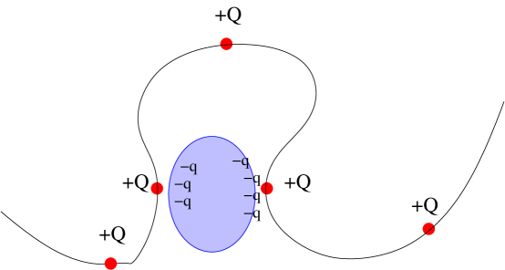
Figure 2: A schematic view of the correlation effect which leads to an effective attraction between like charges on the chain. Opposite charges in the solvent create a region which attracts like charges.

The approach taken in this paper, viz., integrating over the solvent degrees of freedom, is complementary to the approach of Manningmanning , in which the focus rests on the electrostatic potential of the solvent. The polyelectrolyte, represented by an infinite line charge, was shown by Manning to polarize the surrounding ionic solvent. There exists a thin annular cylinder around the rod which attracts counter-ions, allowing for condensation under certain conditions. Manning’s theory is a mean-field approach. The approach developed in this paper is more general. The present theory accounts for fluctuations around the mean-field approximation. It allows for a general description of the physics of polyelectrolytes, and is not restricted to a description of condensation alone.

Furthermore, as suggested earlier, if one takes the segment length $b$ to represent the correlation length of a semi-rigid polymer, we expect the model to reproduce the overall phenomena associated with semi-rigid polyelectrolytes.

IV Regimes of polyelectrolyte behavior

The effective potential derived in the previous section permits an insight into the variety of behavior that polyelectrolytes in solution can display. In order to do that, it is useful to add a constraint to the energy functional described in the previous section, viz., ${\cal F}_{eff}$ to conserve the number of monomers on the polymer:

$$\beta{\cal F}_{eff} \to\beta{\cal F}_{eff}+\beta\Delta{\cal F}_{\mu}$$

$$\beta\Delta{\cal F}_{\mu} =-\mu\int dn\int d^{3}x|\psi(\vec{x},n)|^{2}$$

$$\mu =2\pi N{\ell}_{b}c_{0}(\lambda_{e}^{2}-\lambda^{2}\epsilon^{-1})$$

$${\ell}_{b} =\beta{(q_{+}-|q_{-}|)^{2}}$$ (19)

where $\ell_{B}$ is the Bjerrum length, $c_{0}$ is the number density of monomers, $N$ is the chain length, and the chemical potential is obtained by minimizing the energy functional in Eqn.19 in the limit that the wave amplitude $\psi$ is independent of $\vec{x},~{}n$. It has also been assumed for simplicity that there is a uniform charge distribution along the chain.

By convention, the chemical potential $\mu$ represents the energy required to add a segment to the system. Hence, upon examining Eqn.19, one sees three possible regimes.

Melt: When, $\mu>0$, the polymer behaves as a melt, when repulsion dominates, and it costs energy to add a segment to the system. This occurs when the screening length along the chain $\lambda_{e}>\lambda/\sqrt{\epsilon}$. This is similar to Manning’s discussion of polyelectrolytes.

$\Theta$ point: The monomers are perfectly miscible with each other when the chemical potential $\mu=0$. This occurs when $\lambda_{e}=\lambda/\sqrt{\epsilon}$.

Condensation: When the screening length along the chain $\lambda_{e}<\lambda/\sqrt{\epsilon}$, the chemical potential becomes negative, indicating that the system encourages the addition of monomers. It is natural to identify this regime as that of condensation. Our criterion is similar to that of Manningmanning , but it requires a consideration of fluctuations around the Debye-Huckel approximation. In this sense our approach bears a greater resemblance to the analytic arguments in the paper of Jensen et aljensen .

As discussed earlier in the paper, if we assume that the native charge on the chain is negative, viz., $q_{-}<0$ and corresponds to the charge of a single electron, then clearly, we require $q_{+}$ the charge on the condensed counter-ion to be multi-valent, as otherwise the net charge is null, leading to a neutral polymer, and a discussion of condensation becomes moot. It is beyond the capability of the current theory to address the difference in the condensation behavior of different types of multi-valent molecules carrying the same chargebutler .

Using SAX techniques, Butler et albutler show that virus solutions need a minimum diamine concentration for the onset of condensation, as signaled by the emergence of a peak at a non-zero wave-vector. Moreover, they show that there also exists a maximum ion concentration above which condensation ceases. Equation 19 can be interpreted in light of these experimental results. For low ion concentrations, $q_{+}$ the adsorbed counter-ion charge is correspondingly small, and the screening length along the chain $\lambda_{e}$ is very large. Since the dielectric constant of the aqueous solvent is high ($\sim 80$), the chemical potential $\mu=2\pi N{\ell}_{b}c_{0}(\lambda_{e}^{2}-\epsilon^{-1}~{}\lambda^{2})$ can be greater than zero, preventing condensation. As the ion concentration increases, the screening lengths along the chain and in the solvent decrease. When this change occurs in such a way that $\lambda_{e}$ shrinks faster than $\lambda$, such that $\lambda>\epsilon\lambda$, then the chemical potential $\mu<0$, leading to condensation. Indeed this criterion is similar to the one derived on experimental grounds by Butler et al. For even higher ionic concentrations, $\lambda_{e}$ cannot shrink much below the monomer length, and it is possible for the chemical potential to become positive once again. Condensation then ceases. It may prove possible to adjust the parameters in this theory to reproduce quantitatively the condensation data of Butler et albutler . Our aim here is to display that the theory is simply capable of addressing experiments. The cessation of condensation at relatively high ionic concentration appears to be a new experimental result, and it is important to point out that the theory in this paper can address this issue.

The theory presented in this paper is similar to that of Golestanian and Liverpoolgolestanian . These authors use a phenomenological theory of semi-rigid chains decorated with charges. The only interaction in their theory is that between these charges. The presence of a solvent is implicitly acknowledged through an effective screening length. In our theory, it would correspond to neglecting the terms ${\cal F}_{solvent}$ and ${\cal F}_{polymer-solvent}$. They show that fluctuations in the shape of a semi-rigid rod lead to a buckling instability. These authors too find cessation of condensation upon increasing the salt concentration sufficiently, by considering the behavior of the correlation length.

The current theory can accommodate the zipper-like motif invoked by Kornyshev and Leikenkornyshev . Our approach can be construed as providing an analytic background to the numerical simulations of Stevensstevens of bead and spring polyelectrolytes in a solvent.

The onset of condensation in biopolymers, based on the assumption of entirely rigid polyelectrolytes, has been shown by Kholodenkokholodenko to be analogous to the melting of vortices in Thouless’ two-dimensional model of a glass. In the future, one could attempt to investigate aspect further, using the current formalism, which does not assume rigid rods, as follows. Rather than integrating over the the electrostatic potential of the solvent, one could attempt a functional integration over the polymer degrees of freedom. In this case, extremizing the new effective functional with respect to the electrostatic potential will lead to a generalization of the Kholodenko model to non-rigid polyelectrolytes in solution.

$c_{0}\to 0^{+}$: In addition to the three regimes discussed above, there is one more important regime within the melt phase which merits attention, and permits a connection with the scaling arguments first derived by de GennesdeG1 . Consider the energy density $\beta{f}_{eff}$ for a homogeneous $\psi$:

$$\beta{f}_{eff}=(1/2)N\alpha\hat{V}(k=0)(|\Psi|^{4}-c_{0}|\Psi|^{2})$$ (20)

where $\alpha=\ell_{b}/b$, where the dimensionless number concentration $c_{0}$ can be expressed in terms of the actual monomer number concentration $\tilde{c}_{0}$ and the Kuhn length $b$ as $c_{0}=\tilde{c}_{0}(b/\sqrt{6})^{3}~{}$ Thus when $\tilde{c}_{0}(b/\sqrt{6})^{3}<<~{}1$, one sees that the double-well structure displayed in the next figure is just beginning to form. This is the traditional signal for a second-order phase transition (see Fig.3). Physically this occurs because the mean free path between collisions is very large in the low number concentration limit, permitting large fluctuations, the hall-mark of second order phase transitions. Note that the criterion above encompasses the arguments given by Freed freed , where it is shown that phase transition-like behavior occurs in the $b\to 0$ limit.

Figure 3: A schematic of the double well potential given by the energy density $\beta f_{eff}$, in arbitrary units. Notice that the height of the potential barrier decreases as the concentration of monomers decreases, allowing for more fluctuations between the minima.

V Renormalization Group calculations in the melt regime

We shall now show that the polymer model considered in this paper exhibits a fixed point of the Renormalization Group transformation, reflecting the large fluctuations expected in the $c_{0}b^{3}\to 0^{+}$ (melt) regime. Since a Renormalization Group fixed point in the long wavelength limit (for long chain lengths) is always independent of the details of the interaction, it is expected that our model of realistic interactions should yield results identical to the excluded volume model usually considered in polymer theory. Nevertheless, it is useful to derive this result explicitly so that it displays the validity of the field theoretic approach employed in this paper. Further, we shall compute a reasonably accurate value for the Flory exponent, obtained when the chain length $N$ is very large. In what follows, we shall use a natural system of units, in which the unit of length will be taken to be $b/\sqrt{6}$, where $b$ is the segment length. As discussed earlier in the paper, $b$ is the monomer length for a flexible chain. $b$ could be taken to be the correlation length for a semi-rigid chain.

Finally, note that the model is analogous to the theory of dynamical second order phase transitionshohenberg , with the segment label $n$ playing the role of time. The model has four independent variables, viz., three spatial dimensions and an additional label for the location of a segment along the chain.

Towards that end, let us consider the first order correction to the bare vertex (the basic interaction displayed in Eqn 3). It corresponds to the first order polarization diagram in many-body physics. It represents the generalization of the correction that occurs in an excluded volume interaction modelshirish0 .

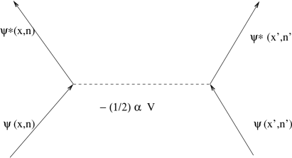
Figure 4: The Feynman diagram indicating schematically the bare vertex, whcih represents the interction term in the energy functional. It displays two segments interacting with each other at a distance.

The result depicted in this figure can be encapsulated as the renormalization of the coupling constant $\alpha$ (using a length scale of $b/\sqrt{6}$):

$$\alpha\to\alpha_{R}(q,\omega) =\alpha~{}(1+\alpha\Pi_{0}(q,\omega)\hat{V}(q))$$

$$\Pi_{0}(q,\omega) =-\int~{}{d^{3}q^{\prime}\over(2\pi)^{3}}~{}\int~{}{d\omega^{\prime}\over 2\pi}~{}\ \hat{G}_{0}(q^{\prime},\omega)~{}\hat{G}_{0}(|\vec{q}~{}^{\prime}-\vec{q}|,\omega^{\prime}-\omega)$$ (21)

where the Fourier transform $\hat{G}_{0}(p,\omega)$ of the unperturbed propagator (Green’s function) defined in Eqn. 1, is given by:

$$\hat{G}_{0}(p,\omega)={1\over-i\omega+p^{2}}$$ (22)

Now $\Pi_{0}(q,\omega)$ represents screening of the interaction between monomers due to intervening segments. Thus it is tacitly assumed that we are in the long-wavelength regime, and the chain length is large, as it is in this regime that one expects screening effects to dominate. Screening is clearly unimportant for extremely short chains, as the probability of finding intervening segments in this case is vanishingly small.

Upon performing the frequency integration in Eqn. 21 by the method of residues, by closing the requisite contour in the lower half-plane:

$$\Pi_{0}(q,\omega)=-~{}\left({2\over(2\pi)^{2}}\right){\cal R}e~{}\left[\int dpp^{2}\int_{-1}^{+1}dx~{}{1\over i\omega-2pqx}\right]$$ (23)

where ${\cal R}e$ implies the real part of the quantity on its right hand side is to be considered. The polarization $\Pi_{0}(q,\omega)$ can be recast as:

$$\Pi_{0}(q,\omega)=-~{}\left({1\over 2\pi^{2}q}\right)\ \int_{0}^{\infty}d\lambda\lambda^{-1}\cos(\omega\lambda)\ \int dpp(\exp(-\zeta p)-\exp(-2pq\lambda))$$ (24)

where $\zeta\to 0^{+}$, and the factor of $\exp(-\zeta p)$ has been inserted into Eqn. 24 to achieve convergence. We now invoke the integral representation of a gamma function, viz., $\int_{0}^{\infty}dxx^{p}\exp(-ax^{m})=m^{-1}a^{-(p+1)/m}\Gamma((p+1)/m)$ to obtain closed form expressions for the integrals in Eqn. 24. However this gives rise to divergent factors such as $\Gamma(-2)$. These divergences can be cured via different methods, such as Wilson’s renormalization scheme. The renormalization scheme to handle ultra-violet divergences utilized in this paper follows more closely the method of dimensional regularizationramond of t’Hooft and Veltman. This technique allows one to separate out the infinities, by setting $p\to p-\epsilon$, $\epsilon\to 0^{+}$, for $p+1/m$ equal to a negative integer, in the expression above for the integral representation of the gamma function.. This allows us to express the polarization function as:

$$\Pi_{0}(q,\omega)={-1\over(2\pi)^{2}q}\zeta^{-2}+{\omega^{2-\epsilon}\over(4\pi)^{2}q^{3}}\Gamma(-2+\epsilon)$$ (25)

Using the Macclaurin series for $\Gamma(-2+\epsilon)$:

$$\Gamma(-2+\epsilon)\approx(1/2)\left(\epsilon^{-1}+\psi(3)+{\cal O}(\epsilon)\right),$$ (26)

one can isolate the divergent portions of the polarization function as being proportional to $\zeta^{-2}$ and $\epsilon^{-1}$. These infinities can be canceled by the invocation of appropriate counter-terms in ${\cal F}$, as is normally done in field theory. This allows us to retain only the finite portion of the polarization function:

$$\Pi_{0}(q,\omega) =-~{}{f(\omega)\over q^{3}}$$

$$f(\omega) =-\left(\omega\over\sqrt{2}\pi\right)^{2}~{}\ \left(\ln(|\omega|)-3/2+\gamma\right)$$ (27)

where $\gamma$ is Euler’s constant, numerically close to $0.5772$.

A test of the renormalization scheme used to handle ultra-violet divergences here is to calculate an observable or a known quantity such as the Flory exponent. This will be done shortly, after a thermodynamic fixed point has been identified. This fixed point is associated with the second order phase transition discussed in the previous.

One must go to the long wavelength limit in order to invoke the Renormalization Group. This Renormalization Group applies to the infra-red limit ($q\to 0$), and must be distinguished from the preceding discussion regarding the behavior in the $q\to\infty$ limit.

It is convenient to redefine a scaled coupling constant in the $q\to 0$ limit, with an associated $\beta$-function which yields the Renormalization Group flow:

$$\hat{\alpha}_{R}(q,\omega) =\alpha_{R}~{}\left({f(\omega)\hat{V}(q=0)\over q^{3}}\right)$$

$$\beta(\hat{\alpha}_{R})\equiv{\partial\alpha_{R}\over\partial\ln L} =3(\hat{\alpha}_{R}-\hat{\alpha}_{R}^{2})$$ (28)

where $q\equiv L^{-1}$. In analogy with the theory of second order phase transitions, scale invariance of the coupling constant must be invoked for a proper description of the physics. It follows from Eqn. 28 that $\beta(\hat{\alpha}_{R})$ has a non-trivial fixed point at $\hat{\alpha}_{R}\equiv\hat{\alpha}_{R}^{*}$, or at $\alpha_{R}\equiv\alpha_{R}^{*}$:

$$\hat{\alpha}_{R}^{*} =1$$

$$\alpha_{R}^{*} ={q^{3}\over f(\omega)\hat{V}(q=0)}$$ (29)

It follows from Eqn.29 that in the long wavelength limit, in the $c_{0}\to 0^{+}$ regime, the interaction has the following universal form, independent of the particular interaction potential we started off with:

$$\alpha\hat{V}(q\to 0)\to-~{}\frac{2\pi^{2}q^{3}}{\omega^{2}\left(\ln(|\omega|)-3/2+\gamma\right)}$$ (30)

The same result could have been obtained in a more mundane fashion by using the so-called Random Phase Approximation (RPA) in which one traditionally sums up bubble diagrams of all orders. Nonetheless, the Renormalization Group approach is essential in that it explicitly manifests the scale invariant properties of the system.

Scaling arguments will be utilized to obtain a value of the Flory exponent. These are provided in lieu of the conventional Renormalization Group argument based on scaling transformations. That treatment is based on the scaling properties of the simpler $\phi^{4}$ Ginzburg-Landau functional. In the present paper, we have a more realistic interaction potential viz., $V$ to deal with. Consequently, the straighforward scaling properties of the $\phi^{4}$ excluded volume theory are no longer valid. A more complex set of scalings, involving the screening lengths are required to maintain the scale invariance of the current theory. But this implies a restriction on the class of polyelectrolytic solutions that can be considered, conforming to the scaling transformations. The alternate derivation offered below suffices to yield the Flory exponent fairly accurately.

Consider scaling behavior of the energy functional for a Gaussian chain:

$$\beta{\cal F}_{0}=\int{d\omega\over 2\pi}~{}\int{d^{3}k\over(2\pi)^{3}}\ \hat{\psi}^{*}(k,\omega)(-i\omega+k^{2})\hat{\psi}(k,\omega)$$ (31)

The diffusion-like, self-similar form permits Functional to be scale invariant under the following transformations:

$$\omega \to\omega/{\cal N}$$

$$k \to k/\xi({\cal N})$$

$$\xi({\cal N}) ={\cal N}^{\nu_{0}}$$

$$\hat{\psi} \to\hat{\psi}\xi^{5/2}({\cal N})$$ (32)

where $\nu_{0}=1/2$. The relation between $\xi$ and ${\cal N}$ is identical to the relation between the radius of gyration $R_{g}$ and $N$. Hence we shall identify the length scale $\xi({\cal N})$ with the radius of gyration.

Let us now consider the case when the interaction viz., $V$ is turned on between the segments. The behavior of the energy functional in the long wavelength limit ($q\to 0,\omega\to 0$) is dominated by the behavior of the effective interaction at the Fixed point of the Renormalization Group transformations (see Eqn.30):

$${\cal F}^{*}\sim\int{d\omega\over 2\pi}~{}\int{d^{3}k\over(2\pi)^{3}}~{}\hat{c}^{*}(k,\omega)~{}\left({k^{3}\over\omega^{2-\pi^{-2}}}\right)~{}\hat{c}(k,\omega)$$ (33)

where we have used $x^{\epsilon}\approx 1+\epsilon\ln x$, $\epsilon<<1$ to convert a logarithm to a power law.

This functional exhibits invariance under:

$$\omega \to\omega/{\cal N}$$

$$k \to k/\xi({\cal N})$$

$$\xi({\cal N}) ={\cal N}^{\nu}$$

$$\hat{\psi} \to\hat{\psi}\xi^{3/2}({\cal N})$$ (34)

where $\nu=2/3-1/(3\pi^{2})\approx 0.63$.

This estimate of the radius of gyration holds for asymptotically large chain lengths $N$, when the concentration of monomers $\tilde{c}_{0}<<(\sqrt{6}/b)^{3}$.

If one accepts the value of $\nu\approx 0.5889$ as obtained within the framework of the Edwards’ model, then the result in this paper is accurate to about $92\%$. On the other hand, H. Kleinertkleinert has shown that when the asymptotic series in the $\epsilon$ expansion is handled appropriately, the value of $0.5889$ is replaced by $3/5$. Kleinert then uses field theoretic methods and the replica trick to rederive a value of $\nu\approx 0.62$. The value we obtained, $\nu\approx 0.63$ is fairly close to the universal value for $\nu\approx 0.634$ accepted in phase transition theory.

This value is quite different from the one derived by Floryflory-el and Katchalskykat for the case of an unscreened Coulomb interaction, which yielded a linear dependence on the chain length.

VI Radius of gyration for short chains

For the case of short chains, when the coupling constant $\alpha=\sqrt{6}{\ell_{b}}/b<1$, one can compute the lowest order Feynman diagram to estimate the self-energy, which renormalizes the Green’s function $\hat{G}_{0}(k,\omega)$. This estimate is correct when $\alpha<1$ and when the chains length is relatively short. This is because screening is expected on physical grounds to be unimportant for short chains. It turns out that there are two terms of ${\cal O}(\alpha)$ in a perturbative expansion of the self-energy. The first one, the tadpole diagram can be renormalized away in the usual fashion by the addition of a counter-term. The remaining term is reminiscent of the exchange diagram in many-electron physics (as shown in Figure5).

Figure 5: A diagrammatic depiction of the approximation used in the calculation. The thick line indicates $\hat{G}$. The first term on the right hand side of the equation refers to $\hat{G}_{0}$. The second term refers to the exchange-like diagram referred to in the text. The final term is the second order correction.

Using the Feynman-Dyson technique, repetitions of this diagram can be summed as a geometric series to infinite order. This exchange diagram contribution to the self-energy can be expressed in closed form as follows:

$$\Sigma_{exch}(k,\omega)=-\alpha\int\frac{d^{3}q}{(2\pi)^{3}}\hat{G}_{0}(k,\omega)\hat{V}(|\vec{k}-\vec{q}|)$$ (35)

where it is tacitly assumed that we are in the low concentration limit. Since our focus is on estimating the radius of gyration for relatively short chains, we need only to evaluate the self-energy in the long-wavelength limit, viz., $k\to 0$. To facilitate this, the angular integrals in Eqn.35 can be done and the contributions to ${\cal O}(k^{2})$ of the integrand can be written explicitly:

$$\int_{0}^{2\pi}~{}d\phi~{}\int_{0}^{\pi}~{}d\theta~{}V(\sqrt{k^{2}+q^{2}-2kq\cos\theta})\approx$$

$$8\,{\pi}^{2}\,\left[\frac{1}{q^{2}+{{{\kappa}_{e}}}^{2}}-\left(\frac{1}{\epsilon\,\left(q^{2}+{\kappa}^{2}\right)}\right)\right]+$$

$$\left(\frac{8\,{\pi}^{2}\,k^{2}}{3}\right)~{}\left[\frac{3}{\epsilon\,{\left(q^{2}+{\kappa}^{2}\right)}^{2}}-\frac{3}{{\left(q^{2}+{{{\kappa}_{e}}}^{2}\right)}^{2}}+q^{2}\,\left(\frac{4}{{\left(q^{2}+{{{\kappa}_{e}}}^{2}\right)}^{3}}-\frac{4}{\epsilon\,{\left(q^{2}+{\kappa}^{2}\right)}^{3}}\right)\right]$$ (36)

The subsequent $k-$integration can be performed with the aid of Mathematica. The results are long and cumbersome and not much is gained by stating the expressions explicitly, other than to say that the integrals contain logarithmic terms of the form $\ln\omega$. Formally, the next step is to evaluate the correlation function:

$${\cal G}(k,N)\approx\int\frac{d\omega}{2\pi}~{}\frac{\exp(-i\omega N)}{-i\omega+k^{2}-\Sigma_{exch}(k,\omega)}$$ (37)

This integral could be evaluated using the method of residues, by closing the contour in the lower half plane if the root(s) of the denominator could be located. Since our interest is in the $k\to 0$ limit, it is possible to estimate the root of the denominator perturbatively:

$$\omega_{root}\approx=-ik^{2}+i\Sigma_{exch}(k,\omega=-ik^{2})+{\cal O}(\alpha^{2})$$ (38)

Before the residue can be calculated, the presence of the logarithmic terms referred to above imply the existence of a branch cut in the complex $\omega$ plane from $-\infty$ to $0$ along the real axis. Hence the contour has to distorted slightly into the lower half-plane along the negative real axis to avoid this branch cut, so that the only singularity enclosed by the contour in the lower half-plane is at the root given by Eqn.38. It then follows, using Mathematica, that in the long wavelength limit:

$${\cal G}(k,N)/{\cal G}(k=0,N) \approx\exp(-ikg(N))$$

$$g(N) =\alpha~{}(\lambda_{e}^{4}-\epsilon^{-1}~{}\lambda^{4})b^{-4}$$ (39)

where $\lambda_{e}$ and $\lambda$ are the screening lengths along the chain and in the solvent, respectively.

The experimentally measurable structure factor can then be evaluated:

$$\hat{S}(k) \approx N(1-(1/3)k^{2}R_{g}^{2}(N)+{\cal O}(k^{4}))$$

$$R_{g} =(b_{effective}/\sqrt{6})~{}N$$

$$b_{effective} =(18\alpha)~{}\left[\left(\frac{\lambda_{e}}{b}\right)^{4}-\epsilon^{-1}\left(\frac{\lambda}{b}\right)^{4}\right]~{}b$$ (40)

Figure 6: Schematic depiction of the linear behavior of the radius of gyration for short chains. Note that the Kuhn length can be shorter than the segment lenght due to a fluctuation effect.

Note that $R_{g}(N)\sim N$ in this regime, as displayed in Fig.6. Moreover, it turns out that $R_{g}(N)$ is extremely sensitive to the parameters in the potential. This is in contrast to the asymptotic regime encountered in the previous section, where universal behavior was found. X-ray or neutron scattering experiments could be performed to test the predictions presented in this section.

One could interpret $b_{effective}$ in Eqn.40 as an effective correlation length and suggest $b_{effective}\to 0$ as a signal for buckling, and hence for condensation. This interpretation is equivalent to the chemical potential considerations presented earlier in the paper, and is similar to the approach of Golestanian and Liverpoolgolestanian .

VII Finite concentration of segments

The discussion in the preceding two sections has been primarily focused on behavior in the melt regime, when the number concentration of segments is vanishingly small. In this case, fluctuations were accounted for, and the radius of gyration for both long and short chains was computed. As the concentration of segments increases, the segments become packed increasingly closer, thereby decreasing fluctuations in the system. Mean field approximations, obtained by extremizing the energy functional can then be invoked to obtain insight into the physics.

In a previous paper,shirish0 which utilized an excluded volume interaction model, we showed how tube-like structures can be obtained. If one restricts attention to obtaining an envelope of structures obtained in the various regimes delineated in section III, then a similar technique provides useful insight in the current approach as well. The basic idea, designed to ease computation, is to replace the short-ranged potential by an effective delta-function pseudo-potential. The effective coupling constant which characterizes the pseudo-potential can be positive or negative, depending on the value of the chemical potential $\mu$. As discussed earlier, the value of the chemical potential is an average way of determining whether the attractive part or the repulsive part dominates the behavior of the system.

The advantage of this method is that it yields the correct average behavior of the system for a reasonably small effort. The disadvantage is that if one is interested in details of the structures which change on the spatial scale less than the one over which the interaction potential varies, then one must resort to vastly more detailed calculations. The approximation consists of the following replacement:

$$(1/2)\alpha\int\int dnd^{3}x~{}dn^{\prime}d^{3}x^{\prime}~{}|\psi(\vec{x},n)|^{2}V(\vec{x}-\vec{x}^{\prime})|\psi(\vec{x}^{\prime},n^{\prime})|^{2}\to$$

$$(1/2)\alpha\hat{V}(k=0)~{}\int dnd^{3}x~{}\int dn^{\prime}~{}|\psi(\vec{x},n)|^{2}~{}|\psi(\vec{x},n^{\prime})|^{2}$$ (41)

Extremization of the functional leads to:

$$({\partial\over\partial n}-\nabla^{2}+\alpha\hat{V}(k=0)|\psi(x,n^{\prime})|^{2}-\mu)\psi(x,n)=0$$ (42)

For cases when the segment label $n$ is not physically relevant, this equation reduces to:

$$(-\nabla^{2}\pm~{}(|\psi(x)|^{2}-1))\psi(x)=0$$ (43)

where the distances are scaled in units of $(b/\sqrt{6})(\alpha|\hat{U}_{Morse}(k=0)|)^{1/2}$, and the amplitude $\psi$ has been scaled by $c_{0}^{-1/3}$ so as to be dimensionless. The positive sign in the non-linear partial differential equation holds when $\mu>0$ in the melt phase, and the negative sign when in the condensed state ($\mu<0$).

Associating $\mu<0$ with a condensed state implies the existence of coherent structures. The first structure we investigate is one in spherical geometry, with a larger amplitude at the center than towards the edges. The ordinary differential equation that requires a solution is:

$$-{1\over r^{2}}~{}{\partial\over\partial r}\left(r^{2}{\partial\psi(r)\over\partial r}\right)-(|\psi(r)|^{2}-1)\psi(r)=0$$ (44)

It turns convenient for numerical purposes to use $y=1/r$, so that Eqn.44 becomes:

$$-y^{4}\Psi^{\prime\prime}(y)-(\Psi(y)^{2}-1)\Psi(y)=0$$ (45)

For $y\to 0$, which is the same as $r\to\infty$, the wave amplitude is expected to decay, so that the non-linear term vanishes, and yields $\Psi(y)=ay\exp(1/y)$. One can now integrate numerically from some $y=y_{minimum}$ to $y=y_{maximum}\equiv r_{minimum}$, adjusting $a$ such that the slope of the amplitude vanishes at $y_{maximum}$. The result is shown in Figure 7.

Figure 7: Displayed is the radial profile of a spherical coherent structure obtained for $\mu<0$. The co-ordinates are dimensionless.

Another interesting structure that we have investigated is a toroidal structure. The interest in this structure arises from the fact that strands of DNA in an ionic solution condense into such shapes under appropriate solvent conditionsgolan ; veena . One may construe the model above (Eqn.43) as an effective model for DNA in solution. The co-ordinate surfaces in toroidal geometry aremargenau : (i) planes through the z-axis, represented by an azimuthal angle, (ii) spheres of varying radii centered up and down the z-axis, and finally, (iii) tores, or anchor rings around the z-axis, labeled by the location of their centers at a distance $a$, and cross-sectional and axial radii $a~{}{\rm csch}\eta$ and $a~{}\coth\eta$ respectively, for $\eta=$ constant, $\eta$ being the toroidal co-ordinate. Since we seek solutions with toroidal symmetry, the only independent variable we need to consider is $\eta$, which leads to a non-linear ordinary differential equation:

$$2\sinh(\eta/2)^{2}(\tanh(\eta/2)\psi^{\prime}(\eta)-2\sinh(\eta/2)^{2}\psi^{\prime\prime}(\eta))-a^{2}(\psi(\eta)^{2}-1)\psi(\eta)=0$$ (46)

The radius $a$ of the torus is determined self-consistently as the value which yields a zero slope but non-zero amplitude at $\eta\to\infty$. This is the center of the doughnut. Again, since we are looking for a doughnut shaped object, it follows that the slope of the function should be zero at a value of $\eta$ at which the cross-sectional radius of the tore is $a~{}{\rm csch}\eta=a$, i.e., when $\eta={\rm arcsinh}1\approx 0.8813$. At this point the the z-axis is a tangent to the tore at the origin, and physical consideration implies a zero slope for continuity. The value of the wave amplitude is taken to be zero at $\eta={\rm arcsinh}1$, i.e., the origin. A shooting method was employed where $a$ was varied iteratively until a solution with a zero slope at $\eta\to\infty$ was obtained numerically. Operationally, the equation was integrated to some large value of $\eta$. The result is displayed as contours in Figure VIII in the $x-z$ plane.. In effect a doughnut shaped structure is obtained, whose hole is partially filled. The energy of this structure is identical to that of the spherical blob displayed in Fig. 7.

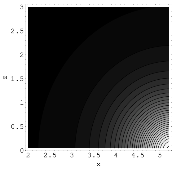
Figure 8: Displayed are the contours of a toroidal structure for $\mu<0$. Note that the doughnut has a profile which indicates a changing density with distance from the center. Note that the width of the structure is approximately unity in dimensionless units.

These are two examples of coherent structures that are possible for $\mu<0$. They are both equally energetically favorable. As such, the approximations employed during these calculations are applicable for large chain lengths, when it is known exoperimentally that either spheroidal or toroidal configurtions are equally likely to occurgolan ; veena . These examples do not constitute an exhaustive list.

Finally, we note from the previous figure, displayed in dimensionless variables, that the width of the toroidal configuration is ${\cal O}(1)$, in the length scale used. Based on this observation, one can calculate the thickness of the toroid for various parameters, and an example is given in Fig. IX. Experiments of the sort performed by Golan et algolan and by Butler et albutler should be able to provide experimental verification of our predictions.

Figure 9: The width of the toroid is plotted in nano-meters for two different cases, as the chain length is varied, for two different screening lengths in the solvent. The upper curve coresponds to a screening lenght of $50b/sqrt6$. The lower curve coresponds to a screening lenght of $10b/sqrt6$.

VIII Conclusion

The theory described in this paper develops a functional integral technique to treat realistic interactions between segments of a polymer in a realistic way, through the use of a finite-ranged repulsive-attractive interaction potential. Examination of the chemical potential led to a classification of homopolymeric systems. It was pointed out that such a classification would be impossible with an a priori excluded volume interaction model. Renormalization Group techniques were used to show that standard concepts in polymer physics are recovered in the limit of low monomer number concentration, for asymptotically long chains, in the melt state. The radius of gyration for extremely short chains is also calculated, and is linear in the chain length, reminiscent of a semi-flexible chain. When the chemical potential is negative, condensed structures are shown to exist, both in spherical as well as toroidal geometry. The predictions that follow from the theory presented in this paper, viz., the short chain radius of gyration, the widths of the toroidal configurations as functions of various experimentally accessible parameters could be verified experimentally.

IX Acknowledgments

I would like to acknowledge useful discussions with Hank Ashbaugh, Tommy Sewell and Kim Rasmussen, and thank Jack Douglas and Enrique Batista for providing useful references.

This work was supported by the Department of Energy Contract no. W-7405-ENG-36.

References

- (1) K. Kroy and E. Frey, Phys. Rev. Lett. 77, 306 (1996).
- (2) E. Frey, K. Kroy, J. Wilhelm and E. Sachmann, e-print cond-mat/9707021, (1998).
- (3) J. Wilhelm and E. Frey, Phys. Rev. Lett. 77, 2581 (1996).
- (4) B. Hinner, M. Tempel, E. Sackmann, K. Kroy, E. Frey, e-print, cond-mat/9712037 (1997).
- (5) J.C. Butler, T. Angelini, J.X. Tang and G.C.L. Wang, Phys. Rev. Lett. 91, 028301-1 (2003).
- (6) J.L. Barrat and J.F. Joanny, arXiv:cond-mat/9601022 (1996).
- (7) W. Kuhn, O. Kunzle and A. Katchalsky, Helv. Chim. Acta 31, 1994 (1948).
- (8) P.G. de Gennes, P. Pincus, R.M. Velasco and F. Brochard, J. Phys. 37, 1461 (1976).
- (9) P.G. de Gennes, Scaling Concepts in Polymer Physics, Cornell University Press, Ithaca, NY (1979).
- (10) J. des Cloizeaux, Phys. Rev. A 10, 1665.
- (11) Y. Oono, Adv. Chem. Phys. LXI, 301 (1985).
- (12) S.M. Chitanvis, Phys. Rev. E 63, 021509 (2001).
- (13) G.H. Fredrickson, V. Ganesan and F. Drolet, Macromol. 35, 16 (2002).
- (14) S.K. Nath, J.D. McCoy, J. P. Donley and J.G. Curro, J. Chem. Phys. 103, 1635 (1995).
- (15) H. Kleinert, Path Integrals in Quantum Mechanics, Statistics and Polymer Physics, World Scientific Publishing Co., Singapore (1990).
- (16) F. Ferrari, Ann der Phys. 11, 255 (2002).
- (17) M. Doi, S.F. Edwards, The Theory of Polymer Dynamics, Oxford University Press, Oxford (1986).
- (18) M. Kaku, Introduction to Superstrings, Springer-Verlag, Berlin (1988).
- (19) G.S. Manning, J. Chem. Phys. 51, 954 (1969).
- (20) N. Gronbech-Jensen, R.J. Mashl, R.F. Bruinsma amd W.M. Gelbart, Phys. Rev. Lett. 78, 2477 (1997).
- (21) R. Golestanian and T.B. Liverpool, Phys. Rev. E 66, 051802 (2002).
- (22) A.A. Kornyshev and S. Leiken, Phys. Rev. E 62 2576 (2000).
- (23) M.J. Stevens and K. Kremer, Phys. Rev. Lett. 71, 2228 (1993).
- (24) A.L. Kholodenko and A.L. Beyerlein, Phys. Rev. Lett., 74, 4679 (1995).
- (25) P.C. Hohenberg and B.I. Halperin, Rev. Mod. Phys. 49, 435 (1977).
- (26) P. Ramond Field Theory: A Modern Primer, Benjamin Cummings Pub. Co., Inc., Reading, MA (1981).
- (27) K.F. Freed, Renormalization Group Theory of Macromolecules, John Wiley and Sons, N.Y. (1987).
- (28) R. Golan, L.I. Pietrasanta, W. Hsieh and H.G. Hansma, Biochem. 38, 14069 (1999).
- (29) V. Vijayanathan, T. Thomas, A. Shirahata and T.J. Thomas, Biochem. 40, 13644 (2001).
- (30) H. Margenau and G.M. Murphy, The Mathematics of Physics and Chemistry, Van Nostrand Reinhold Co. (1956).