Distribution of equilibrium edge currents

Abstract

We have studied the distribution of equilibrium edge current density in 2D system in a strong (quantizing) magnetic field. The case of half plane in normal magnetic field has been considered. The transition from classical strong magnetic field to ultraquantum limit has been investigated. We have shown that the edge current density oscillates and decays with distance from the edge. The oscillations have been attributed to the Fermi wavelength of electrons. The additional component of the current smoothly depending on the distance but sensitive to the occupation of Landau levels has been found. The temperature suppression of oscillations has been studied.

The magnetic field acting on the low dimensional system is traditionally considered as homogeneous and coinciding with the external field. Nevertheless, the magnetization of such quantum system as atom substantially changes the magnetic field in the vicinity of nucleus. This is essential for some phenomena, e.g., NMR. The distribution of magnetic field in the systems with spatial quantization have been studied by authors in papers [1] using the linear approximation in an external field. This problem is close to the problem of orbital magnetism intensively investigated in different systems with separable and non-separable variables [2, 3, 4]. It was shown, that the susceptibility of a large system at low temperature strongly fluctuates and changes the sign when the Fermi level moves between the energy levels of the system.

The goal of the present paper is to study the spatial distribution of equilibrium currents in 2D semi-infinite plane sample subjected to a strong magnetic field. Such mathematical setting is applicable for a sample of arbitrary shape if its characteristic dimensions exceed the inverse cyclotron diameter.

Edge current in 2D system in a finite magnetic field.

Let us consider a semi-infinite plane $x>0,~{}~{}-\infty<y<\infty$, with hard border in a magnetic field $B_{z}=B$. Assume the vector potential has gauge $A_{y}=Bx$. The states in the presence of magnetic field can be described by the longitudinal momentum $p$ and the transversal number $n$: $\psi_{n,~{}p}(x)e^{ipy}$. Here and below $\hbar=1$. The wave functions can be expressed via the parabolic cylinder function $D_{\nu}(x)$:

$$\psi_{n,p}(x)=CD_{\nu_{n}}\left(\sqrt{2}\left(x-x_{p}\right)/a\right),~{}~{}~{}~{}~{}C^{2}\int\limits_{-x_{p}}^{\infty}D_{\nu_{n}}\left(\sqrt{2}x/a\right)dx=1.$$ (1)

Here $a=\sqrt{c/eB}$ is the magnetic length, $x_{0}=-pa^{2}$. The boundary condition $D_{\nu_{n}}(-\sqrt{2}pa)=0$ determines the energy levels $E_{n,p}=\omega(\nu_{n}(p)+1/2)$, $n=0,1...$; $\omega=eB/m_{e}c$ is the cyclotron frequency, $m_{e}$ is the electron effective mass.

The density of current has the form

$$j_{y}(x)=\frac{j_{0}}{2\pi}\sum_{n=1}^{\infty}\int\limits_{-\infty}^{\infty}dpa[\left(x_{p}-x\right)\psi_{n,p}^{2}(x)\bigl{(}f_{+}+f_{-}\bigr{)}$$

$$+\frac{gm_{e}}{2m_{0}}\bigl{(}f_{-}-f_{+}\bigr{)}\frac{a^{2}\partial\psi_{n,p}^{2}(x)}{\partial x}],$$ (2)

where $j_{0}=e\omega/a=e/(m_{e}a^{3})$ is the characteristic current density, $f_{\pm}=f(E_{n}(p)\pm g\mu_{B}B/2)$,   $f(E)=(\exp{((E-\mu)/T)}+1)^{-1}$ is the Fermi distribution function ($\mu,\ T$ are the chemical potential and temperature, correspondingly), $g$ is the $g$-factor. The expression (2) contains two contributions caused by the orbital and spin parts of the current (the first and the second lines, correspondingly). Below we shall neglect the spin term, assuming the smallness of the $g$-factor.

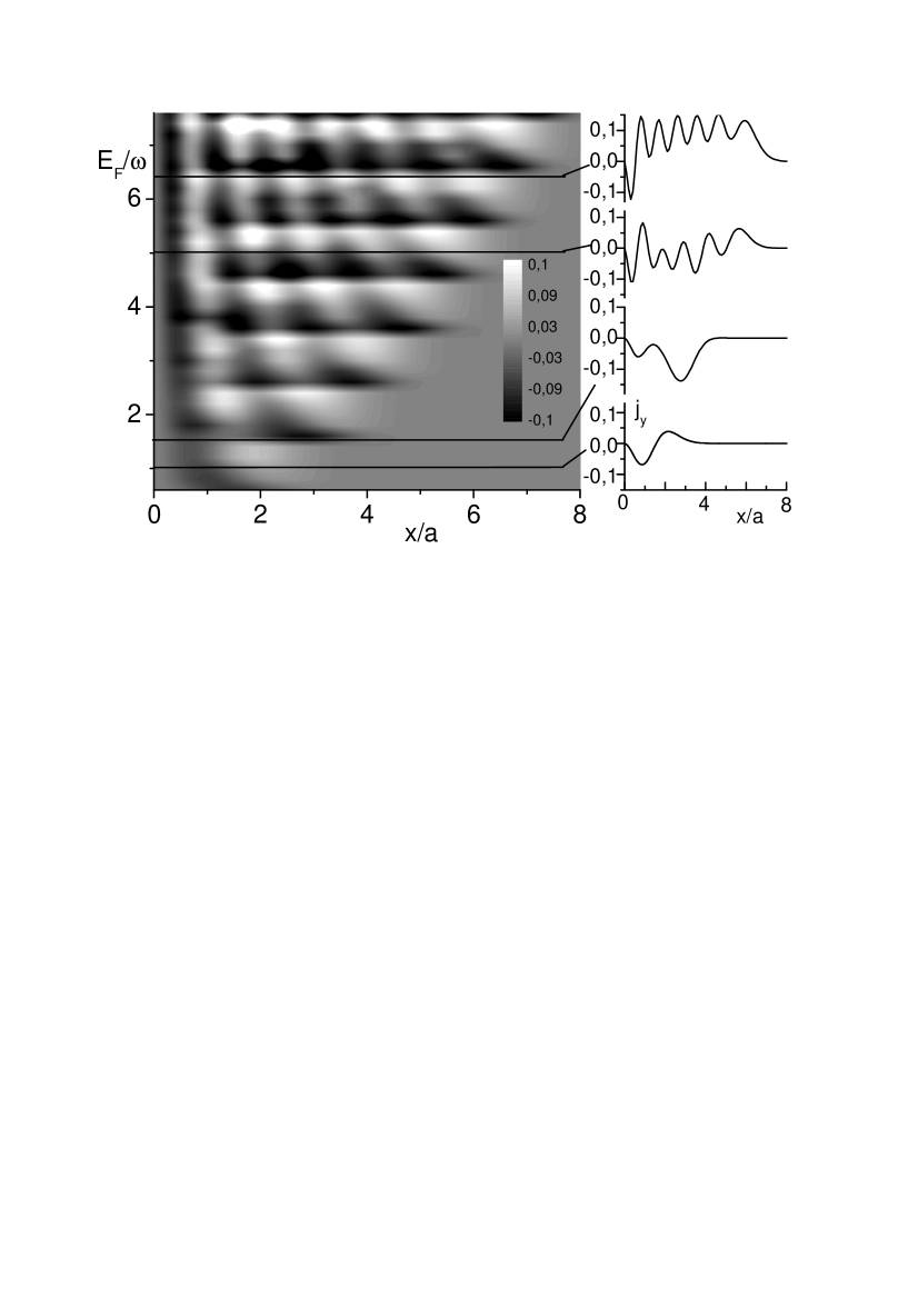
Figure 1: On the left: relief of the edge current density in units $j_{0}$ at finite magnetic field as function of the distance from the border and Fermi energy. The grey color corresponds to zero density of a current, white - positive, black - negative. On the right: dependence of the current density on distance at the selected Fermi energy (marked by straight lines in the left figure).

Plots of the edge current calculated according to Eqs.(1) and (Edge current in 2D system in a finite magnetic field.) are presented in Figs.1-3. Let us discuss behavior of the edge current at low temperature. The direction of the current is determined by the vector product of the normal and the magnetic field. However, it does not mean the constancy of the sign of the surface current density. Really, let only one Landau level be occupied. Consider the states localized far from the boundary. These states are not perturbed by the wall. The contribution to the current density from one state with given $p$ is antisymmetric relative to the point $x_{p}$. As the state approaches to the boundary the level goes up. Occupied levels (they lie under Fermi level) have close wave functions. Averaging over momentum compensates the current density far from the point of intersection the Fermi level with Landau level, while near this point noncompensated contribution of constant sign (positive in this instance) remains. When the Fermi level approaches the lowest Landau level, the distance of the edge state from the border grows as $\ln^{1/2}(\mu/\omega-1/2)$ and the edge state becomes more and more ideal. Under increase of Fermi level the wave function begins to distort due to boundary, positive part of the contribution to the average current density is suppressed but the negative contribution appears and the graph of current density acquires negative minimum.

Crossing next Landau levels results in new contributions to the current density. First these contributions are situated on large distance from the boundary, then they move to it and merge with contributions from lower lying states. The upper is the state the wider is the region it occupies and the more oscillations it contributes to the current density. When we have many occupied Landau levels, the contributions from different levels merge to produce the Friedel oscillations of surface current density studied by authors earlier [1]. However, the number of oscillations is restricted (unlike earlier considered limit of weak magnetic field), because the surface current is distributed on the thickness of the order of cyclotron diameter $2r_{c}$. Within this region the current density oscillates, on the outside it decays exponentially. The number of oscillations is defined by the number of occupied Landau levels. In the region $x\ll 2r_{c}$ the effect of magnetic field is weak and the linear-response expression from [1] is valid.

As it is seen from Fig.2 the smooth dependence on coordinate $x$ is superimposed on the space oscillations. The total edge current $J$ experiences the alternating-sign oscillations with magnetic field. These oscillations accord with the de-Haas-van Alphen oscillations of magnetic moment.

Note that in the limit of weak magnetic field the smooth contribution transforms to studied in [1] contribution depending linearly on the distance, and oscillations decaying on power law spread to infinite range from the boundary.

Temperature suppresses the oscillations of current density (see Fig.2). It happens more effectively on large distance from boundary. The suppression takes place due to temperature dephasing of electrons near the Fermi surface on characteristic length $l_{T}=k_{F}/(2\pi m_{e}T)$, where $k_{F}$ is the Fermi momentum [1]. At finite magnetic field the competition of two lengths which cut down oscillations (cyclotron diameter and $l_{T}$) occurs. The scattering suppress both spatial oscillations and smooth contribution as well.

The alternating-sign oscillations of total edge current seem at first sight strange if to take into account, that at large Fermi energy the total edge current should be diamagnetic and be described by the formula

$$J=-\frac{j_{0}a}{12\pi}.$$

However, in the limit of the large system the total quantity of edge current $J$ is directly connected to the magnetic moment of the system by the relation $M=JS/c$, where $S$ is the system area. At the same time, the total moment at $T=0$ can be found using $\Omega$-potential of the system

$$M=-\frac{\partial\Omega}{\partial B}=\frac{j_{0}aS}{\pi c}\sum\limits_{n=0}\left[\frac{\mu}{\omega}-\left(2n+1\right)\right]\theta\left(\mu-\left(n+\frac{1}{2}\right)\omega\right).$$ (3)

This expression oscillates with $\mu$, jumping when the Fermi energy crosses the Landau levels. In accord with this formula the moment vanishes when the Fermi energy lies in the middle between the Landau levels.

On the other hand, the edge currents in nonequilibrium conditions are connected with the quantization of microcontact resistance in adiabatic transport regime of quantum Hall effect. The total current in the state $(n,p)$ is given by expression

$$j_{n,p}=-e\frac{\partial E_{n,p}}{\partial p}.$$ (4)

As the states are localized on $x$, the edge current is determined by the states with $x_{p}$, lying near to the border. The partial current density $j_{n,p}$ exponentially decreases with increase of $x_{p}$. Therefore, summing currents over all states near the border we obtain finite quantity. Such reasons determine the quantization of microcontact resistance.

The total edge current in semi-infinite problem at $T=0$ looks like

$$J=-e\sum\limits_{n,p}\frac{\partial E_{n,p}}{\partial p}~{}\theta\left(\mu-E_{n}(p)\right)=-\frac{j_{0}a}{\pi}\sum\limits_{n=0}\left[\left(n+\frac{1}{2}\right)-\frac{\mu}{\omega}\right]\theta\left(\mu-\left(n+\frac{1}{2}\right)\omega\right).$$ (5)

The current through the structure is expressed via the difference of the edge currents (5), corresponding to chemical potentials of edges $\mu_{1}$ and $\mu_{2}$. The difference $\mu_{1}-\mu_{2}$ in a nonequilibrium problem coincides with the potential difference $V$, applied to the microstructure. From here we conclude, that the nonequilibrium current is

$$J=e^{2}VN/h.$$

The chemical potentials of edges are equal in equilibrium, but the edge current from one edge should be determined by the same expression, as in non-equilibrium. However, such understanding of the Eq.(5) contradicts Eq.(3) for the magnetic moment and numerical calculations.

To find out the nature of the discrepancy, we shall find the contribution to current density for the boundless problem from Landau levels with a momentum lying between $p_{1}$ and $p_{2}$, where $|x_{p_{1}}-x_{p_{2}}|\gg a$

$$j_{y}(p_{1},p_{2};x)=-\frac{j_{0}}{\pi}\sum\limits_{n}\int\limits_{p_{1}}^{p_{2}}\left(x-x_{p}\right)\varphi_{n}^{2}\left(\frac{x-x_{p}}{a}\right)dp=-\frac{j_{0}}{\pi}\sum\limits_{n}(\int\limits_{-\infty}^{p_{2}}dp...-\int\limits_{-\infty}^{p_{1}}dp...).$$ (6)

Here $\varphi_{n}(\xi)$ are dimensionless normalized functions of the harmonic oscillator. Contributions from regions close to the points $x_{p_{1}}$ and $x_{p_{2}}$ are independent and separated in the space. Two edge currents are presented in Eq.(6)(and can be isolated), but cancel each other in the total current. The resulting contribution to a total edge current from current density near the point $x_{p_{1}}$ is located far from border and should be subtracted from a total edge current.

This part of a current is determined by integration of $j_{y}(p_{1},p_{2};x)$ with respect to $x$ near the point $x_{p}$

$$\int\limits_{x_{p}-\Delta}^{x_{p}+\Delta}j_{y}(p_{1},p_{2};x)dx=\frac{j_{0}a}{\pi}\sum\limits_{n=0}^{\infty}\left(n+\frac{1}{2}\right)\theta\left(\mu-\left(n+\frac{1}{2}\right)\omega\right).$$ (7)

Here $\Delta\gg a\sqrt{N}$. Subtracting (7) from (5) we obtain the correct expression for a total edge current $J=Mc/S$, with $M$ from the (3). Numerical calculations (see Fig. 3) accord with this formula.

Conclusions.

The presence of edge current results in weak change of a magnetic field applying to the 2D system. The non-uniformly distributed current creates the non-uniformly distributed magnetic field.

Note that the spatial inhomogeneity of a magnetic field can effect on any responses sharply dependent on a magnetic field, in particular, on the Shubnikov oscillations, geometrical resonances or magnetic focusing. One can expect that the inhomogeneity will result in washout of sharp singularities in these quantities. This gives the way to measure the magnetization.

Other variants can be based on sensitivity of nuclear spins to a local magnetic field. NMR-markers, placed on the certain atomic planes, can act as indicators of local magnetic fields. One can propose to use the constant in time magnetic field for shift of NMR line or alternating magnetic field for excitation of transitions. The temporal change of inhomogeneous magnetic field can be produced by control of the electron wave functions due to alternating gate voltage. As another way one can suggest the periodic change of temperature of electron gas by source-drain voltage with subsequent change of $\delta B$) caused by the temperature suppression of the Friedel oscillations.

Figure 2: Dependence of density of edge current on temperature. The Fermi level is close to the 5th Landau level: solid curves  -  $E_{F}=4.4\omega$, dotted curves  -  $E_{F}=4.6\omega$; in these cases the integrated currents are oppositely directed. At temperatures $T\gg|E_{F}-4.5\omega|$ the curves merge. At $T\gg\omega$ the current density ceases to depend on a magnetic field.

Figure 3: The total edge current as function of a magnetic field at $T=0$ calculated from Eq.(2) (dotted) and from Eq.(3) (solid).

References

- [1] L.I. Magarill, M.M. Mahmoodian, and M.V. Entin, JETP Lett. 75, 470 (2002); M.V. Entin, L.I. Magarill, and M.M. Mahmoodian, Proceedings of 10th International Symposium ”Nanostructures: Physics and Technology”, 237 (2002); M.V. Entin and M.M. Mahmoodian, ibid. 290; M.V. Entin, L.I. Magarill, M.M. Mahmoodian, cond-mat/0204159.
- [2] M.Ya. Azbel. Phys.Rev. B 48, 4592-4598(1993).
- [3] K. Richter, D. Ullmo, and R.A. Jalabert. Phys. Rep. 276, 1-83(1996).
- [4] E. Gurevich and B. Shapiro. J.Phys. I France 7, 807-820(1997).