Wave Packet Propagation and Electric Conductivity of Nanowires

1 Introduction

In general, transport phenomena are intimately related to the dynamics of particles involved. In the case where the direct interaction between the particles that participate in the transport process are negligible, the solution of of the one-particle time-dependent Schrödinger equation contains all information, at least in principle. Of course, the same information is obtained by solving the corresponding stationary problem. Appealing features of the time dependent approach are its conceptual simplicity, its flexibility in terms of system geometry and choice of (spin-dependent) scattering potentials, and its absolute numerical stability. On the other hand, in contrast to the time independent approach, it is not well established how to extract the transport coefficients from the time dependent data.

Recently, the electric conductance in nanoscale wires has attracted much interest.${}^{\hbox{\immediate{\bf{?}})}}$ In particular, the effect of the magnetic domain wall in ferromagnetic substances on the conductance has been studied extensively. The effect of a magnetic domain wall on the conductivity was clearly observed in experiments on nanowires.${}^{\hbox{\immediate{\bf{?}},\penalty 1000\hskip 0.91003pt plus 0.70004pt minus 0.70004pt{\bf{?}},\penalty 1000\hskip 0.91003pt plus 0.70004pt minus 0.70004pt{\bf{?}},\penalty 1000\hskip 0.91003pt plus 0.70004pt minus 0.70004pt{\bf{?}},\penalty 1000\hskip 0.91003pt plus 0.70004pt minus 0.70004pt{\bf{?}},\penalty 1000\hskip 0.91003pt plus 0.70004pt minus 0.70004pt{\bf{?}})}}$ In these experiments, the field is initially applied along the wire direction and the magnetization uniformly aligns ferromagnetically in this direction, where the conductance is that of the wire with uniform magnetization. If the magnetic field is reversed, then the anti-domain of the magnetization appears at the edge of the wire. The appearance of the anti-domain creates a domain wall. The applied field is not very strong and hence only one domain wall exists. The anti-domain grows in time and finally the total magnetization is reversed. The resistance decreases shortly after the field is reversed and after some period returns to its initial value. This period corresponds to the life time of the domain wall.${}^{\hbox{\immediate{?},\penalty 1000\hskip 0.91003pt plus 0.70004pt minus 0.70004pt{?})}}$

This phenomenon has been analyzed theoretically by various methods.${}^{\hbox{\immediate{\bf{?}},\penalty 1000\hskip 0.91003pt plus 0.70004pt minus 0.70004pt{\bf{?}},\penalty 1000\hskip 0.91003pt plus 0.70004pt minus 0.70004pt{\bf{?}},\penalty 1000\hskip 0.91003pt plus 0.70004pt minus 0.70004pt{\bf{?}},\penalty 1000\hskip 0.91003pt plus 0.70004pt minus 0.70004pt{\bf{?}},\penalty 1000\hskip 0.91003pt plus 0.70004pt minus 0.70004pt{\bf{?}},\penalty 1000\hskip 0.91003pt plus 0.70004pt minus 0.70004pt{\bf{?}},\penalty 1000\hskip 0.91003pt plus 0.70004pt minus 0.70004pt{\bf{?}},\penalty 1000\hskip 0.91003pt plus 0.70004pt minus 0.70004pt{\bf{?}})}}$ One approach is to use the Kubo formula. Tatara and Fukuyama${}^{\hbox{\immediate{?})}}$ pointed out that the existence of the domain wall causes the decrease of the resistance due to the quantum effect, which is in contradiction with the intuitive, classical picture that the current would be scattered with the domain wall. The key point is that the system has impurities which provide the resistivity of the medium and the domain wall suppresses the scattering by the impurities when the spins of electrons change adiabatically with the change of the magnetization.

It is interesting to observe how the electron propagate through the magnetic domain and how it is scattered microscopically. This physical picture was investigated by a direct method, i.e. by a direct simulation of electron wave packet propagation in a system with impurities and the magnetic domain wall.${}^{\hbox{\immediate{?})}}$ We will call this approach ‘wave packet method’. This direct method provides intuitively understandable information about the electron propagation.

We could also extract information for the transport coefficient from the simulation. The conductance is naively related to the amount of the probability to go through the domain, which can be regarded as the transmission coeffient. This quantity was studied to investigate the above problem of the conductance of nanowires with the domain wall, and the result supports the enhancement of the conductance (decrease of the resistance).${}^{\hbox{\immediate{?})}}$ In this work, the conductivity is estimated by studying the propagation of a simple wave packet. However, the transmission coefficient is usually defined for the incoming plane wave instead of a wave packet. Actually, in the wave packet method, we have to specify the initial configuration of the wave packet.

As shown below, we find that the transmission coefficient depends on the initial configuration of the packet. Therefore it is difficult to extract the conductivity from data obtained in a single initial configuration. Not only the quantitative amount but also qualitative features change with the initial configuration of the packet. Thus, we study how much information for the transport coefficient we can obtain by the wave packet method.

In order to obtain the reference data for given systems we calculate the conductivity by direct numerical evaluation of the Kubo formula. In this paper, we mainly study the dependence of the conductivity on the width of the domain wall. We find that, in the case without the magnetic domain walls, the transmission coefficients obtained by the wave packet method with various initial configurations show common qualitative features. In this case we do not need an additional procedure to extract the qualitative features of the conductivity from the simulation data.

However, as mentioned above, when the domain wall is present, the transmission coefficient strongly depends on the initial configuration, e.g., various shapes of wave packets and spin polarizations. Under this circumstance, we need an additional procedure to obtain the conductance from the simulation data. Inspired by the Landauer formula, we propose a procedure to estimate the conductance from the transmission coefficient data for various initial configurations.

We study in detail the dependence of the conductance on the width of the domain wall in some small systems for which the direct numerical calculation of the Kubo formula is feasible. In such small systems, different configurations of the random potential lead to large fluctuation of the dependence. Our procedure successfully reproduces the individual results.

We also study the effect of the width of the wave packets in the direction of the propagation, discuss its relation to the damping factor in the Kubo formula and find that quantum interference plays an important role.

Applying this method we also study the conductivity in the domain wall system. Qualitatively similar results are obtained by the wave packet method and the direct numerical evaluations of the Kubo formula. In this perturbative regime, our results agree with those of Tatara and Fukuyama.${}^{\hbox{\immediate{?})}}$

2 Time-Dependent Schrödinger Equation for Propagation of Wave Packet

The electron propagation in the nanowire is described by the time-dependent Schrödinger equation${}^{\hbox{\immediate{\bf{?}},\penalty 1000\hskip 0.91003pt plus 0.70004pt minus 0.70004pt{\bf{?}})}}$

$$i\hbar{\partial\over\partial t}\Psi_{\sigma}(t)=\left[-{\hbar^{2}\over m^{2}}\nabla^{2}+V(\mbox{\boldmath$r$})-\mu_{B}\vec{\sigma}\cdot\mbox{\boldmath$M$}(\mbox{\boldmath$r$})\right]\Psi_{\sigma}(t),$$ (2.1)

where $\sigma(=\uparrow$ or $\downarrow$) is the spin of the electron, $m$ is the mass, and $V(\mbox{\boldmath$r$})$ denotes spin-independent impurity potential. Here $\mbox{\boldmath$M$}(\mbox{\boldmath$r$})$ is the magnetization of the medium, $\vec{\sigma}$ is the Pauli matrix denoting the spin of the electron and $\vec{\sigma}\cdot\mbox{\boldmath$M$}(\mbox{\boldmath$r$})$ represents the magnetic coupling between them.

For numerical work, it is convenient to use dimensionless quantities. First we express the energy in unit of the Fermi energy $E_{\rm{F}}$, a typical energy scale of the system. Using

$$\vec{r}^{\prime}=\frac{\vec{r}}{\hbar/\sqrt{2mE_{F}}},\quad t^{\prime}=\frac{t}{\hbar/E_{\rm{F}}},$$ (2.2)

we have

$$i\frac{\partial\Psi^{\prime}}{\partial t^{\prime}}=\left\{-\nabla^{\prime}\;{}^{2}+V^{\prime}-\vec{\sigma}\cdot\vec{M}^{\prime}\right\}\Psi^{\prime}\equiv{\cal{H}^{\prime}}\Psi^{\prime},$$ (2.3)

where $\Psi^{\prime}(\vec{r}^{\prime},t^{\prime})\equiv\Psi(\vec{r},t)$, $M^{\prime}\equiv M(\vec{r}^{\prime})$, $V^{\prime}\equiv V(\vec{r^{\prime}})$. Hereafter, in our numerical work, we use renormalized quantities, i.e. we express the energy in units of $E_{\rm{F}}$ ($\epsilon\equiv E/E_{\rm{F}}$), distances in units of $x_{0}=\hbar/\sqrt{2mE_{\rm{F}}}\equiv 1/k_{\rm{F}}\equiv\lambda_{\rm{F}}/{2\pi}$ ($x^{\prime}=x/x_{0}$), and momentum in units of $p_{0}=\hbar k_{\rm{F}}=\sqrt{2mE_{\rm{F}}}$ ($p^{\prime}=p/p_{0}$) and drop the primes in the notation. Writing the wave function in the form of the spinor

$$\Psi\left(\vec{r},t\right)=\left(\begin{array}[]{@{}c@{}}\psi_{\uparrow}\left(\vec{r},t\right)\\ \psi_{\downarrow}\left(\vec{r},t\right)\end{array}\right),$$ (2.5)

Eq.(2.1) reads

$$i\frac{\partial}{\partial t}\left(\begin{array}[]{@{}c@{}}\psi_{\uparrow}\\ \psi_{\downarrow}\end{array}\right)=\left[-\nabla^{2}+\left(\begin{array}[]{@{}cc@{}}V&0\\ 0&V\end{array}\right)-\left(\begin{array}[]{@{}c@{}c@{}}M_{z}&M_{x}-iM_{y}\\ M_{x}+iM_{y}&-M_{z}\end{array}\right)\right]\left(\begin{array}[]{@{}c@{}}\psi_{\uparrow}\\ \psi_{\downarrow}\end{array}\right).$$ (2.6)

For time evolution

$$\psi\left(\vec{r},t_{0}+\tau\right)=e^{-i\cal{H}\tau}\psi\left(\vec{r},t_{0}\right),$$ (2.7)

we use the method of exponential decomposition up to the second order

$$e^{x(A+B)}=e^{xA/2}e^{xB}e^{xA/2}.$$ (2.8)

Here we take

$$\begin{array}[]{lll}A&=&-{\hbar^{2}\over 2m}\nabla^{2}\\ B&=&-\mu_{B}\vec{\sigma}\cdot\vec{M}(\vec{r})+V(\vec{r}),\end{array}$$ (2.9)

where at each position $\vec{r}$, $A$ and $B$ are $2\times 2$ matrices. For most calculations we used the second order decomposition and, as a check, we occasionaly used the fourth order algorithm.${}^{\hbox{\immediate{\bf{?}})}}$

In our numerical simulation, we use a real-space representation of the wave function. The wave function is given by its value at points of the lattice and the value of the spin. For example, in two dimensions, we divide the space into $N_{x}\times N_{y}$ cells and each cell is identified by the coordinate $(i,j)$. Thus the wave function can be represented as

$${\Psi\left(x,y,t\right)=\left(\begin{array}[]{c}\psi_{\uparrow}\left(1,1,t\right)\\ \psi_{\uparrow}\left(1,2,t\right)\\ \vdots\\ \psi_{\uparrow}\left(N_{x},N_{y},t\right)\\ ,\\ \psi_{\downarrow}\left(1,1,t\right)\\ \psi_{\downarrow}\left(1,2,t\right)\\ \vdots\\ \psi_{\downarrow}\left(N_{x},N_{y},t\right)\\ \end{array}\right)}.$$ (2.10)

The wave function at cell $(i,j)$ is given by $\Psi_{\sigma}(i,j,t)$. We use several formulae to approximate $\nabla^{2}$. For example, the standard 3-point formula in one direction reads

$${\partial^{2}f\over\partial x^{2}}\approx{f_{i-1,j}-2f_{i,j}+f_{i+1,j}\over\Delta^{2}}+O(\Delta^{3}),$$ (2.11)

where $\Delta$ is a mesh size. We also use the 5-point formula

$$\frac{\partial^{2}f}{\partial x^{2}}\approx\frac{-f_{i+2,j}+16f_{i+1,j}-30f_{i,j}+16f_{i-1,j}-f_{i-2,j}}{12\Delta^{2}}+O{\left(\Delta^{5}\right)},$$ (2.12)

and the 9-point formula

$$\frac{\partial^{2}f}{\partial x^{2}}+\frac{\partial^{2}f}{\partial y^{2}}\approx\frac{\left\{\begin{array}[]{@{\,}c@{\;}r@{\;}l@{\;}c@{\;}r@{\;}l@{\;}c@{\;}r@{\;}l@{\;}}&&f_{i-1,j+1}&+&4&f_{i,j+1}&+&&f_{i+1,j+1}\\ +&4&f_{i-1,j}&-&20&f_{i,j}&+&4&f_{i+1,j}\\ +&&f_{i-1,j-1}&+&4&f_{i,j-1}&+&&f_{i+1,j-1}\end{array}\right\}}{6\Delta^{2}}+O{\left(\Delta^{4}\right)}.$$ (2.13)

We used Eq.(2.13) in this paper. In order to avoid the reflection from the edges of the system, we used absorbing boundary conditions at both edges. As for the impurity potential, we randomly distribute the impurity sites where $V(\vec{r})\neq 0$ with some concentration at each cell.

The quantity of interest in this work is the conductance through the wire. In the wave packet method we compute the transmission coefficient, and convert it to the conductance from it. We determine the transmission coefficient by measuring the electron current through a virtual screen, as indicated in Fig.1. The total current in the $x$-direction is given by

$$\int j\left(x,y,t\right)dy=-\frac{i\hbar}{2m}\left\{\psi^{*}\frac{\partial}{\partial x}\psi-\left(\frac{\partial}{\partial x}\psi^{*}\right)\psi\right\}.$$ (2.14)

The transmission coefficient $T$ is calculated from the amount of current through the right-most detection screen. Likewise the reflection coefficient $R$ is calculated from the amount of current that goes through the left-most detection screen.

In Fig.$2$, we show an example of electron propagation. Initially, we prepare a wave packet moving from left to right with the group velocity. Then it is scattered by the impurities. Part of the wave is reflected and some part crosses the impurities region and is transmitted through the wire. Intensity arriving at the ends of the wire is being absorbed. Note that even after a fairly long time (see Fig.2 (f)), we find some intensity in the impurity region.

3 Relation between the transmission coefficient and the conductance

3.1 Sensitive dependence on the initial configuration

The conductance $\sigma$ is related to the transmission coefficient $T$ through the Landauer formula $\sigma=T/(1-T)$. The transmission coefficient $T$ is obtained by solving the scattering problem for an incoming plane wave. However, in the wave-packet method we cannot use the plane wave. Therefore, to obtain $T$, we solve the Schrödinger equation for a specific initial configuration, and study the dependence on the initial configurations,

As initial configurations, we use the rippled-Gaussian wave-packet

$$\psi_{\rm rG}(\vec{r},n)\equiv\sqrt{\frac{2}{\sigma_{x}L_{y}}}\frac{1}{\pi^{1/4}}e^{ik_{x}x}e^{-(x-x_{0})^{2}/2{d_{x}}^{2}}\sin\left(\frac{n\pi y}{L_{y}}\right)$$ (3.1)

with $k_{y}=1,2,3$ and 4, for both $\sigma=\uparrow$ and $\downarrow$. Thus we have 8 different initial configurations. The shapes of $k_{y}=1,2,3$ and 4 are depicted in Fig.3. For each $n$, we determine the value of $k_{x}$ such that $\langle\psi^{*}_{\rm{rG}}|{\cal H}|\psi_{\rm{rG}}\rangle=E_{\rm F}$.

For the eight initial configurations, we compare the transmission coefficients in a system with one magnetic domain wall $M(x,y)$ with some random positions of impurity $V(x,y)$,

$$M_{x}(x,y) = M_{0}\mathop{\rm sech}\nolimits\left(\frac{x-x_{0}}{\lambda_{w}}\right)$$ (3.2)

$$M_{z}(x,y) = M_{0}\mathop{\rm tanh}\nolimits\left(\frac{x-x_{0}}{\lambda_{w}}\right),$$ (3.3)

where $M_{0}$, $x_{0}$, and $\lambda_{w}$ denote the height, the position of the center, and the width of the magnetic domain wall, respectively. If the transmission coefficient is insensitive to the initial configuration we may obtain information for the conductance from one simulation. In the presence of a magnetic potential, however, we find that the transmission coefficient is very sensitive to the initial configuration. In Fig.4 we show the dependence of the transmission coefficients on the width of a single domain wall. We find that each initial configuration results in very different transmission coefficients not only quantitatively but also qualitatively. That is, some increase with the width and others decrease. Thus we have to be careful to deduce properties of the conductance from the data of the transmission coefficients, and we need some statistical treatment.

3.2 Comparison with the Kubo formula

In order to check the results, we calculate the conductivity by the Kubo formula for the system with a given configuration of impurity potential and magnetization. The method is described in the Appendix. In this approach we need to obtain all eigenvalues and eigenvectors of the system, and therefore we can only treat small system up to $256\times 16$. Although we can calculate much larger systems by the wave-packet method, in order to compare with results of the numerical study of the Kubo formula, we study the same $256\times 16$ system by the wave-packet method. Here in the wave packet method, the region of $256\times 16$ is assigned to the scattering region as shown in Fig. $1$, and we attached the extra region of $208\times 16$ as leads at both ends of scattering region.

First we compare the results for the case without magnetic domain wall. In Fig.5, we show the dependence of the Drude formula (solid line), and the formula (dashed line) that includes the weak localization correction obtained by a perturbative treatment of the Kubo formula ${}^{\hbox{\immediate{?})}}$

$$\sigma_{0}=\frac{e^{2}n\tau}{m}-\frac{2e^{2}}{\pi\hbar\Omega}\sum_{q}\frac{1}{q^{2}}=\frac{e^{2}}{h}n\lambda_{\rm{F}}l\left(1-\frac{\lambda_{\rm{F}}}{l}\frac{2}{\pi^{3}}\frac{L_{x}}{L_{y}}\right),$$ (3.4)

where $n$ denotes the electron density, $\tau$ is the scattering time ($\tau^{-1}={2\pi}n_{i}|v|^{2}n/\hbar$, where $n_{i}$ is the density of the impurities and $|v|$ is the strength of the impurity potential), $l\equiv(\hbar k_{\rm{F}}\tau/m)$ is the mean free path, and $(L_{x},L_{y})$ is size of the system. The first term in the right hand side of Eq.(3.4) corresponds to the Drude formula. In Fig.5 we plot the data obtained numerical study of the Kubo formula (closed circle) and those obtained by the wave packet method with $n=1$, 2, 3 and 4 (cross, asterisk, open square, and closed square, respectively). These data do not depend on the spin. We find that all of them qualitatively agree with each other.

3.3 Effects of magnetic potential

When the magnetic potential is introduced, as we saw in Fig.4, the data vary strongly with the initial configurations. Thus we need some method to extract information of the conductance from the data. In order to obtain the conductivity by the Kubo formula, periodic boundary conditions are required. A single domain wall is not compatible with periodic boundary conditions. Therefore, for simplicity, we adopt a screw shaped magnetic potential to study the effect of magnetic scattering:

$$M_{x}(x,y) = M_{0}\frac{\tanh(\frac{x-x_{0}}{\lambda_{w}})}{\cosh(\frac{x-x_{0}}{\lambda_{w}})}$$ (3.5)

$$M_{z}(x,y) = \pm M_{0}\sqrt{1-\left\{\frac{\tanh(\frac{x-x_{0}}{\lambda_{w}})}{\cosh(\frac{x-x_{0}}{\lambda_{w}})}\right\}^{2}},$$ (3.6)

where ${M_{x}}^{2}+{M_{z}}^{2}={M_{0}}^{2}$, $M_{0}$, $x_{0}$, and $\lambda_{w}$ denote the height, the position of the center, and the width of the screw structure, respectively. The magnetization of the constant strength $M_{0}$ rotates in the $x-z$ plane. Here $M_{0}$ is taken to be $0.2E_{\rm F}$.

3.4 Transmission coefficient and conductivity

Now we describe the statistical procedure that we use to process the numerical data obtained for different initial wave packets. In the spirit of the Landauer formula, different initial configurations may correspond to different channels. The transmission coefficients vary from channel to channel, and therefore the dependence of the transmission on the initial states appears in a natural way. Let $T_{ij}$ be the transmission coefficient from the mode $i$ to $j$, and let $R_{ij}$ be the reflection coefficient from the mode $i$ to $j$. Because we cannot distinguish between outgoing channels we sum up all the outgoing channels. We define the transmission and reflection coefficients for the incoming channel $i$ by

$$T_{i}=\sum_{j}T_{ij},\qquad R_{i}=\sum_{j}R_{ij}.$$ (3.7)

Following Azbel et al.,${}^{\hbox{\immediate{\bf{?}})}}$ the conductance is given by

$$G=\frac{2e^{2}}{h}\sum_{i}T_{i}\frac{2\sum_{i}{v_{i}}^{-1}}{\sum_{i}(1+R_{i}-T_{i}){v_{i}}^{-1}},$$ (3.8)

where $v_{i}={\hbar k_{i}/m}$. As to the incident modes, we take the eight modes used above ($k_{y}=1,2,3,$ and 4 and $\sigma=\uparrow$ and $\downarrow$).

We study eight samples of the system with different impurity configurations. As we mentioned, for each sample, the results depend sensitively on the initial state. Thus, we use the formula (3.8) for each sample with the eight initial configurations (3.1). We obtain the conductance as a function of the width of the magnetic potential $\lambda_{w}$. In Fig.6, we compare the results of the present method with those obtained by the numerical treatment of the Kubo formula. The data are normalized by the conductance of the system without magnetic domain wall in order to see the effect of the domain wall. After the processing of (3.8), the data show roughly similar behavior. For example, if we look at the data for the sample of impurity-1, the conductance decreases a little and then increases with the width. The sample of impurity-3 shows monotonic decrease with the width, etc..

The data in Fig. 6 depend strongly on the impurity configuration. We believe that this strong dependence is due to the smallness of the system. We find that the Kubo formula systematically gives larger normalized values, the reason why is under investigation now.

4 Quantum interference and conductance

In this section, we study the effect of the width $d_{x}$ of the initial packet along the $x$ direction. If the width is small, then the wave function is localized in the $x$ direction and is spread out in momentum space. If the width is large then the wave packet is nearly a plane wave and the the quantum mechanical interference among spatially distant places is important. The width $d_{x}$ corresponds to the damping factor in the Kubo formula $\epsilon$ (see Appendix A) in the sense that it causes decoherence in the system.${}^{\hbox{\immediate{\bf{?}})}}$ The small damping factor corresponds to small $d_{x}$.

In Fig. 7 and Fig. 8, we show the domain wall width dependence of the conductance for three values of $\epsilon$ and $d_{x}$, respectively. We find that the renormalized conductance is close to one in the strongly decoherent cases (Fig.7(c) and Fig.8(c)). This means that the effect of the domain wall becomes small as the decoherent effect increases. Thus we confirm that the intrinsic scattering by the magnetic potential requires a kind of quantum interference effect. Indeed, the increase of the conductivity in the presence of a magnetic domain wall has been interpreted as an effect of adiabatic motion (quantum mechanical coherent motion) of the electron in the magnetic potential.${}^{\hbox{\immediate{?})}}$

5 Effects of the magnetic domains on the conductance

Making use of the present method, let us study the effect of magnetic domain wall on the conductance in a wire. The structure of the magnetization profile is given by

$$M_{x}(x)=M_{0}{\rm sech}\left(\frac{x-x_{0}}{\lambda_{w}}\right),$$ (5.1)

$$M_{z}(x)=M_{0}\tanh\left(\frac{x-x_{0}}{\lambda_{w}}\right).$$ (5.2)

Tatara and Fukuyama have calculated analytically the Kubo formula for the conductance by a perturbation theory.${}^{\hbox{\immediate{?})}}$ They found

$$\sigma=\frac{e^{2}}{h}nl\lambda_{\rm{F}}\left[1-\frac{1}{2\pi^{2}}\frac{{\lambda_{\rm{F}}}^{2}}{\lambda_{w}L_{x}}-\frac{2}{\pi^{2}}\frac{\lambda_{\rm{F}}}{l}\left(\frac{L_{w}}{L_{y}}\tan^{-1}\frac{L_{x}}{\pi L_{w}}\right)\right],$$ (5.3)

where $L_{w}\equiv\sqrt{D\tau_{w}}$, $D\equiv\hbar^{2}\ k_{\rm{F}}^{2}\tau/2m^{2}$, $\tau=lm/\hbar k_{\rm{F}}$, and $\tau_{w}\equiv 24\pi^{2}\lambda_{w}L_{x}(\mu_{B}M_{0})^{2}\tau/(\lambda_{\rm{F}}E_{\rm{F}})^{2}$.

We study this problem by the wave packet method and a numerical evaluation of the Kubo formula. For this purpose we again use a periodic boundary condition and we set a pair of domain walls in the system.

For the numerical calculation we use a $256\times 16$ lattice, corresponding to a physical size of $45\lambda_{\rm{F}}\times 2.8\lambda_{\rm{F}}$. Periodic boundary conditions are used. The impurity concentration is $n_{i}=4.88\%$, $V_{0}=8.3E_{\rm{F}}$, $M_{0}=0.2\sim 0.4E_{\rm{F}}$, the temperature is set to $E_{\rm{F}}/60$, and $\epsilon=4.17\times 10^{-4}E_{\rm{F}}$. We study eight different impurity configurations and we plot the average of the results. The standard deviation of the data is about $0.1$. The data strongly depend on the samples. This may be due to the smallness of the system. We find that the numerical data show the enhancement of the conductance, in agreement with the analytical results for the single domain wall, as shown in Fig.9.

6 Summary and Discussion

We have studied the conductivity of systems with magnetic domain walls and impurity potential by direct numerical calculations of the time-dependent Schrödinger equation for the propagation of the electron wave packet (wave-packet method). We found that, when the system has magnetic domain walls, the transmission of the wave-packet depends sensitively on the initial configuration. We have proposed a method of a statistical treatment of data in the spirit of the multi-channel Landauer formula to obtain the electric conductivity from various initial configurations of the wave packets. In order to validate the method, we compare the results with the results obtained by direct numerical calculations of the conductivity by the Kubo formula. We conclude that the wave-packet method in combination with the statistical treatment is a useful approach to obtain information on the conductivity.

We applied the method to a system with a ferromagnetic domain wall, and found that the analytical estimation of Kubo formula, numerical calculated Kubo formula and the wave-packet model consistently show the enhancement of conductivity in the magnetic domain wall.

In the present work, we mainly concentrate on the comparison between the results of Kubo formula and the wave-packet method. A numerical evaluation of the Kubo formula requires a lot of computer memory because we use the simple $L^{3}$ method, where $L$ is a size of the system. Memory and CPU time of the wave-packet method increase linearly with $L$ and therefore it can be used for much large systems and for various boundary conditions. For instance, preliminary calculations for the three-dimensional case have been carried out. The results of the present study show sensitive dependence on the positions of the impurities. This may be attributed to the small size of the system whereas in large lattices we expect self-averaging of the conductivity.

The authors would like to thank Dr. Gen Tatara for valuable discussions. The present work is partially supported by the Grant-in-Aid from the Ministry of Education. The calculation is done at the supercomputer center of ISSP.

Appendix: Direct calculation of the Kubo formula

The dc conductivity can be obtained from the Kubo formula,

$$\sigma_{0} = \frac{\pi\hbar}{\Omega}\left(\frac{e}{m}\right)\int\,dE\,\left(-\frac{df(E)}{dE}\right)\sum_{\alpha,\alpha^{\prime}}\langle\alpha|p_{x}|\alpha^{\prime}\rangle\langle\alpha^{\prime}|p_{x}|\alpha\rangle\delta\left(E-E_{\alpha}\right)\delta\left(E-E_{\alpha^{\prime}}\right),$$ (6.1)

where $|\alpha\rangle$ and $E_{\alpha}$ are the $\alpha$-th eigenstate and eigenvalue for the Hamiltonian, and $f(E)$ is the Fermi distribution.

In the Kubo formula approach, a non-zero current can be realized by adopting periodic boundary conditions. Eigenstates and eigenvalues are obtained by a direct numerical diagonalization of the system Hamiltonian.

In a numerical approach, we must use a finite system, taking finite grids in real space, which leads to discretized energy levels. In this case, it is convenient to introduce the Lorenzian smoothing for the delta function in (6.1):

$$\delta(x)\sim\frac{\epsilon}{x^{2}+\epsilon^{2}},$$ (6.2)

with small $\epsilon$. In case of $\epsilon\rightarrow 0$, the conductivity vanishes due to the discreteness of the eigenvalues. In the present study, we take $\hbar\epsilon$ to be the same order of energy spacing $\Delta E$:

$$\hbar\epsilon\sim\Delta E.$$ (6.3)

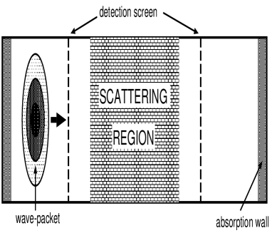
Fig.  1: Simulation model

M. Maeda, K. Saito, S. Miyashita, H. De Raedt

$$\begin{array}[]{ccc}\epsfbox{F10.eps}&\epsfbox{F55.eps}&\epsfbox{F100.eps}\\ {\rm(a)}&{\rm(b)}&{\rm(c)}\\ \epsfbox{F150.eps}&\epsfbox{F200.eps}&\epsfbox{F400.eps}\\ {\rm(d)}&{\rm(e)}&{\rm(f)}\end{array}$$

Fig.  2: 2d-picture of the probability distribution: (a)$t=10$, (b)$t=55$ ,(c)$t=100$,(d)$t=150$, (e)$t=200$ and (f) $t=400$.

M. Maeda, K. Saito, S. Miyashita, H. De Raedt

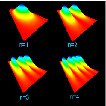
Fig.  3: Probability distributions of the initial configurations for $k_{y}=1,2,3$ and 4 in Eq.(3.1)

M. Maeda, K. Saito, S. Miyashita, H. De Raedt

Fig.  4: Dependence on the different initial configuration of the transmission coefficient as a function of the domain-wall width. Each symbol represents the data for different initial condition.

M. Maeda, K. Saito, S. Miyashita, H. De Raedt

Fig.  5: Comparison of the transmission coefficients and conductivity. Kubo formula (solid line), Kubo formula with the effect of localization (dashed line), Kubo formula numerical method (closed circle), and the wave packet method with $n=1,2,3$, and $4$ (cross, asterisk, open square, and closed square, respectively).

M. Maeda, K. Saito, S. Miyashita, H. De Raedt

Fig.  6: Normalized conductance as obtained by the Kubo formula (a), and the wave-packet method (b). Different symbols represent data for different random potentials, using the same symbols in (a) and (b) for the same random potential.

M. Maeda, K. Saito, S. Miyashita, H. De Raedt

Fig.  7: Dependence on $\epsilon$ of the normalized conductance $\sigma/\sigma_{0}$. (a):$\epsilon=4.17\times 10^{-4}$E_F,(b): $\epsilon=8.33\times 10^{-4}$E_F,(c):$\epsilon=4.71\times 10^{-3}$E_F. Different symbols represent data for different random potentials, using the same symbols in (a), (b) and (c) for the same random potential.

M. Maeda, K. Saito, S. Miyashita, H. De Raedt

Fig.  8: Dependence on $d_{x}$ of the normalized conductance $\sigma/\sigma_{0}$. (a): $d_{x}=3.54\lambda_{\rm F}$,(b): $d_{x}=2.12\lambda_{\rm F}$,(c):$d_{x}=0.71\lambda_{\rm F}$. Different symbols represent data for different random potentials, using the same symbols in (a), (b) and (c) for the same random potential.

M. Maeda, K. Saito, S. Miyashita, H. De Raedt

Fig.  9: Comparison between the analytical (solid line) and the numerical results of the Kubo formula () and wave packet method().

References

- [1] M. N. Baibich, J. M. Broto, A. Fert, F. Nguyen Van Dau, F. Petroff, P. Eitenne, G. Creuzet, A. Friedrich and J. Chazelas: Phys. Rev. Lett. 61 (1988) 2472.
- [2] M. Viret, D. Vignoles, D. Cole, J. M. D. Coey, W. Allen, D. S. Daniel and J. F. Gregg: Phys. Rev. B 53 (1996) 8464.
- [3] J. F. Gregg, W. Allen, K. Ounadjela, M. Viret, M. Hehn, S. M. Thompson and J. M. D. Coey: Phys. Rev. Lett. 77 (1996) 1580.
- [4] U. Ruediger and J. Yu and S. Zhang and A. D. Kent and S. S. P. Parkin: Phys. Rev. Lett. 80 (1998) 5639.
- [5] K. Hong and N. Giordano: J. Phys. Condens. Matter 10 (1998) L401.
- [6] Y. Otani, K. Fukamichi, O. Kitakami, Y. Shimada, B. Pannetier, J. P. Nozieres, T. Matuda and A. Tonomura: Proc. MRS Spring Meeting (San Francisco, 1997) 475 215 (1997).
- [7] Y. Otani, S. G. Kim, K. Fukamochi, O. Kitamich and Y. Shimada: IEEE Trans. Magn. 34 (1998) 1096.
- [8] G. Tatara and H. Fukuyama, Phys. Rev. Lett. 78 (1997) 3773, G. Tatara: J. Mod. Phys. B 15 (2001) 321.
- [9] P. A. E Jonkers, S. J. Pickering, H. De Raedt and G. Tatara: Phys. Rev. B 60 (1999) 15970.
- [10] P. M. Levy and S. Zhang, Phys. Rev. Lett. 79 (1997) 5110.
- [11] A. Brataas and G. Tatara and G. Bauer, Phys. Rev. B 60 (1999) 3406.
- [12] J.B.A.N. van Hoof, K. M. Schep, A. Brataas, G. Bauer and P. J. Kelly, Phys. Rev. B 59 (1999) 138.
- [13] G.Tatara, Y.-W.Zhao, M. Muñoz and N. García: Phys. Rev. Lett. 83 (1999) 2030.
- [14] P. Grokom and A. Brataas and G. E. W. Bauer: Phys. Rev. Lett. 83 (1999) 4401.
- [15] H. Imamura and N. Kobayashi and S. Takasaki and S. Maekawa: Phys. Rev. Lett. 84 (2000) 1003.
- [16] N. García, M. Muñoz and Y. W. Zhao: Phys. Rev. Lett. 82 (1999) 2923.
- [17] H. De Raedt and K. Michielsen, Computer in Physsics, 8 (1994) 600.
- [18] H. De Raedt, Annual Reviews of Computational Physics IV, ed. D. Stauffer, World Scientific, 107 (1996).
- [19] M. Ya. Azbel, J. Phys. C14 (1985) L225.
- [20] R. Kubo: J. Phys. Soc. Jpn 12(1957) 570.
- [21] R. Landauer: IBM J. Res. & Dev. 1 (1957) 223, R. Landauer: Z. Phys. B, Condens. Matter 68 (1987) 217, M. Büttiker, Y. Imry, R. Landauer and S. Pinhas: Phys. Rev. B 31 (1985) 6207, M. Ya. Azbel: J. Phys. C 14 (1985) L225.
- [22] M. Suzuki, J. Phys. Soc. Jpn. 61 (1992) 3015.
- [23] Y. Imry and N. Shiren: Phys. Rev. B 33 (1996) 7992.