Dynamics of a magnetic moment induced by a spin-polarized current

Abstract

Effects of an incoming spin-polarized current on a magnetic moment are explored. We found that the spin torque occurs only when the incoming spin changes as a function of time inside of the magnetic film. This implies that some modifications are necessary in a phenomenological model where the coefficient of the spin torque term is a constant, and the coefficient is determined by dynamics instead of geometrical details. The precession of the magnetization reversal depends on the incoming energy of electrons in the spin-polarized current. If the incoming energy is smaller than the interaction energy, the magnetization does not precess while reversing its direction. We also found that the relaxation time associated with the reversal depends on the incoming energy. The coupling between an incoming spin and a magnetic moment can be estimated by measuring the relaxation time.

I introduction

Tremendous attention has been paid to the dynamics of magnetization in recent years because this problem is of fundamental importance in understanding magnetism and because the problem is of interest to technological applications in magnetic devices.hillebrands One of intriguing features of magnetization motion is spin transfer from a spin-polarized current to a magnetization of a ferromagnetic film, theoretically proposed by Slonczewskislonczewski and Bergerberger , and later experimentally verified.myers ; katine Since this spin transfer mechanism was first conceptualized, many studiesbazaliy ; sun ; waintal ; stile ; zhang have been performed on this phenomenon. However, the dynamics of a magnetic moment driven by a spin-polarized current has not been fully explored.

In this paper we investigate the current-driven precession and reversal of a magnetic moment. This is done quantum mechanically using a simple Hamiltonian, without introducing an external magnetic field. In this way one can easily distinguish contributions from the current from those induced by an externally applied field. To this end, we describe the motion of a magnetic moment in the lab frame where details of the magnetization reversal are best illustrated. Since dynamics of a magnetic moment can be formally described in the local moment frame and such a description may also give some intuition about the dynamics, we examine an interaction between a spin-polarized current and a magnetic moment in the local frame at the Hamiltonian level in section (II). Then dynamics in the lab frame is illustrated in section (III). In this section one can see details of the dynamics such as under what conditions the motion of the magnetization can be non-precessional or the relaxation time associated with the reversal is a minimum. These phenomena have not been explored in the literature so far. Section (IV) is devoted to discussions about the adiabatic approximation used to describe the motion of a magnetic moment, and we close with a summary.

II Formalism in the local moment frame

To describe effects of an incoming spin current on a magnetic moment ${\bf M}$, as in Ref.bazaliy one can choose a frame $(X^{\prime}Y^{\prime}Z^{\prime})$, where ${\hat{z}}^{\prime}$ is parallel to ${\bf M}$. Such a frame is called the local magnetic moment frame. Extensive work on ferromagnetism in the local moment frame has been done in Ref.koreman An advantage of this frame is that it is trivial to diagonalize an interaction between an incoming spin ${\bf s}$ and a magnetic moment: $-2J_{H}{\bf M}\cdot{\bf s}$, where $J_{H}$ is the coupling.

Let us start with a simple Hamiltonian relevant to the interaction:

$$H=\int{}dx\left[\psi^{+}_{\alpha}(x)\left(-\frac{\nabla^{2}}{2m}\right)\psi_{\alpha}(x)-2J_{H}{\bf M}(x)\cdot{\bf s}+V(x)\psi^{+}_{\alpha}(x)\psi_{\alpha}(x)\right]$$ (1)

where $\psi^{+}_{\alpha}(x)$ creates an electron with a spin $\alpha$ at $x$, $m$ is the electron mass and $V(x)$ is an impurity potential. The magnitude of the magnetic moment is $M_{0}$, which remains unchanged. The electron spin can be represented as $s^{i}=(1/2)\psi^{+}_{\alpha}\sigma^{i}\psi_{\beta}$, where $\sigma^{i}$ is a Pauli matrix with $i=x,y$ and $z$. We assume that the magnetic moment is determined by a localized electron $\Psi$ so that the kinetic part of the localized electron is not included in the Hamiltonian.

Suppose a local magnetic moment ${\bf M}({\bf x})$ points in the direction $(\theta,\;\phi)$ at ${\bf x}$ as seen in Fig. 1. Then, a local rotation ( or coordinate transformation to the local moment frame) is introduced: $\psi_{\alpha}(x)=U_{\alpha\beta}(x)\chi_{\beta}(x)\;,$ where

$$U(x)=\left(\begin{array}[]{cc}\cos(\theta/2)e^{-i\phi/2}&-\sin(\theta/2)e^{-i\phi/2}\\ \sin(\theta/2)e^{i\phi/2}&\cos(\theta/2)e^{i\phi/2}\end{array}\right)\;.$$ (2)

In terms of $\chi(x)$, the Hamiltonian can be written as

$$H=\int{}dx\left[\frac{1}{2m}\nabla\left(\chi^{+}_{\beta}U^{+}_{\beta\alpha}\right)\cdot\nabla\left(U_{\alpha\gamma}\chi_{\gamma}\right)-J_{H}\chi^{+}_{\beta}U^{+}_{\beta\alpha}({\bf M}\cdot\sigma_{\alpha\mu})U_{\mu\nu}\chi_{\nu}+V(x)\chi^{+}_{\alpha}\chi_{\alpha}\right]$$ (3)

Since the interaction term in the Hamiltonian is diagonalized in this $\chi(x)$ basis, we obtain

$$H=H_{0}+\int{}dx\left[{\bf A}_{\alpha\beta}\cdot{\bf j}_{\alpha\beta}+A^{(0)}_{\alpha\beta}\rho_{\alpha\beta}\right]\;,$$ (4)

where

$$H_{0} = \int{}dx\left[\chi^{+}_{\alpha}(x)\left(-\frac{\nabla^{2}}{2m}\right)\chi_{\alpha}-J_{H}M_{0}\chi_{\alpha}\sigma^{z}_{\alpha\beta}\chi_{\beta}+V(x)\chi^{+}_{\alpha}(x)\chi_{\alpha}(x)\right]$$

$${\bf j}_{\alpha\beta} = \frac{1}{2im}\left[\chi^{+}_{\alpha}\nabla\chi_{\beta}-(\nabla\chi^{+}_{\alpha})\chi_{\beta}\right]\;,\hskip 14.22636pt{\bf A}_{\alpha\beta}=-iU^{+}_{\alpha\gamma}(\nabla U_{\gamma\beta})\;,$$

$$A^{(0)}_{\alpha\beta} = \frac{1}{2m}(\nabla U^{+}_{\alpha\gamma})\cdot(\nabla U_{\gamma\beta})\;,\hskip 14.22636pt\mbox{and}\hskip 14.22636pt\rho_{\alpha\beta}=\chi^{+}_{\alpha}\chi_{\beta}\;.$$

After diagonalizing the interaction, we have an extra term $H^{\prime}=\int{}dx\left[{\bf A}_{\alpha\beta}\cdot{\bf j}_{\alpha\beta}+A^{(0)}_{\alpha\beta}\rho_{\alpha\beta}\right]$ in Eq. (4) instead of off-diagonal terms of the interaction in Eq. (1). Using the explicit form of $U(x)$, we can calculate vector potentials $A^{(0)}_{\alpha\beta}$ and ${\bf A}_{\alpha\beta}$. This was the route followed in Ref.bazaliy , which led to a monopole-like term in the energy. Those authors attributed the spin torque term to this new vector potential, which is purely geometrical.

Here we follow a different route, since we are interested in a simpler case, where the magnetization is not a function of position. Thus, in our case of a single-domain ferromagnet, the extra term shown above will disappear because $\nabla U=0$. Instead, our spin torque will be present due to the dynamics of the coupled spin-moment system. In addition, we will not require an assumption regarding the magnitude of $J_{H}$ in order to proceed, and we will utilize an impurity potential for convergence purposes which is otherwise irrelevant to the spin transfer as in Ref.bazaliy

Figure 1: Geometry of a quantum mechanical problem associated with the spin transfer. The incoming electron to the positive $X$ axis are spin-polarized along ${\hat{z}}$ axis. The ferromagnet surface is at $x=0$ and parallel to $YZ$ plane. The direction of the magnetic moment is defined by $\theta$ and $\phi$, which are functions of time $t$. The ferromagnet is assumed to be sufficiently thick.

III Dynamics of a magnetic moment in the lab frame

A disadvantage of the description in the local moment frame is that the precession of the magnetic moment cannot be seen; in other words, a precessional reversal of the magnetic moment cannot be distinguished from a plain reversal. Since our goal in this paper is to investigate the dynamics of the magnetic moment as mentioned in the introduction, we describe the motion of the magnetic moment in the lab frame. The geometry of our problem is shown in Fig. 1. We assume a single-domain ferromagnet in the $YZ$ plane for simplicity and consider the Hamiltonian Eq.(1). The incoming spin is along ${\hat{z}}$ and the direction of the magnetic moment is defined by $\theta(t)$ and $\phi(t)$, which vary as functions of time $t$.

The equation of motion for the magnetic moment ${\bf M}$ can be obtained quantum mechanically: $d{\bf M}/dt=i\left[H,{\bf M}\right]$. Since $M^{i}=(1/2)\gamma_{0}\Psi^{+}_{\alpha}\tau^{i}_{\alpha\beta}\Psi_{\beta}$, where $\Psi$ and $\tau^{i}$ are the operator and a Pauli matrix for localized electrons, respectively, and $\gamma_{0}$ is the gyromagnetic ratio, the equation becomes

$$\frac{d{\bf M}}{dt}=2\gamma_{0}J_{H}\left({\bf M}\times{\bf s}\right)\;.$$ (5)

To analyze this equation we consider ${\bf M}$ as a classical vector and take ${\bf s}$ as its expectation value over the ferromagnet. If we decompose ${\bf s}$ into a parallel ${\bf s}_{\parallel}$ and a perpendicular ${\bf s}_{\perp}$ component to ${\bf M}$, we know that only ${\bf s}_{\perp}$ contributes to the equation. We can express ${\bf s}_{\perp}$ using any unit vector. Let us choose, for the unit vector, the initial direction of the incoming spin ${\hat{s}}_{0}={\hat{z}}$. Then

$${\bf s}_{\perp}=s_{\perp}({\hat{M}}\times{\hat{s}}_{0})+s^{\prime}_{\perp}\left[{\hat{M}}\times({\hat{s}}_{0}\times{\hat{M}})\right]\;,$$ (6)

where $s_{\perp}=\frac{{\hat{s}}_{0}\cdot({\bf s}\times{\hat{M}})}{1-({\hat{s}}_{0}\cdot{\hat{M}})^{2}}$ and $s^{\prime}_{\perp}=\frac{{\hat{s}}_{0}\cdot{\bf s}-({\hat{s}}_{0}\cdot{\hat{M}})({\bf s}\cdot{\hat{M}})}{1-({\hat{s}}_{0}\cdot{\hat{M}})^{2}}$. Using Eq. (6), we can rewrite Eq. (5) as follows:

$$\frac{d{\bf M}}{dt}=-2\gamma_{0}J_{H}s_{\perp}{\bf M}\times({\hat{s}}_{0}\times{\hat{M}})+2\gamma_{0}J_{H}s^{\prime}_{\perp}({\bf M}\times{\hat{s}}_{0})\;.$$ (7)

As we can see in the above equation, the first term on the right hand side gives the spin torque while the second term causes a precession of the magnetic moment. We emphasize that the spin torque occurs only when ${\bf s}(t)$ changes as a function of time $t$. If ${\bf s}$ remains parallel to ${\hat{s}}_{0}$, then $s_{\perp}$ vanishes and no spin torque takes place. In this instance, the effect of a spin is the same as that of an external magnetic field along ${\hat{z}}$ and the magnetic moment precesses. In a phenomenological model,sun the spin torque is represented by ${\bf M}\times({\hat{s}}_{0}\times{\hat{M}})$ with a proportional constant. However, a time dependence of $s_{\perp}$ is crucial as we emphasized. We also should stress that $s_{\perp}$ and $s^{\prime}_{\perp}$ are determined by dynamics, not geometrical details as in Ref.zhang

To evaluate the expectation value of ${\bf s}$, we need to solve the Schrödinger equation for the Hamiltonian Eq. (1). Basically, the equation is one-dimensional because of translational symmetry in the $YZ$ plane. We choose the direction of the polarized spin to be ${\hat{z}}$. Then, an incoming wave function $|\psi_{in}\rangle$ with a momentum ${\bf k}$ or an energy $\epsilon=k^{2}/2m$ is $|+\rangle e^{ikx}$, where $|+\rangle$ is the spin-up state in the lab frame. We need to consider a normalization factor $C$ for $|\psi_{in}\rangle$. Since this wave function describes an electron beam, $|C|^{2}$ is the number of electrons $N_{e}$ per unit length in one dimension. Intuitively, the more electrons are bombarded into the ferromagnet, the stronger is the effect of spin transfer. We thus expect the time scale for the reversal to scale inversely with $N_{e}$ (the more the number of electrons, the faster the moment responds). Similarly, the time scale will be proportional to the magnitude of the local spin, $S_{local}\;(=M_{0}/\gamma_{0})$ (the larger the moment, the longer it will take to reverse it).

The reflected $(|\psi_{re}\rangle)$ and transmitted $(|\psi_{tr}\rangle)$ wave functions are eigenstates $|\chi_{\uparrow}\rangle$ and $|\chi_{\downarrow}\rangle$ of the interaction $2J_{H}{\bf M}\cdot{\bf s}=J_{H}{\bf M}\cdot{\bf\sigma}\;$; namely, $J_{H}{\bf M}\cdot{\bf\sigma}|\chi_{\uparrow}\rangle=J_{H}M_{0}|\chi_{\uparrow}\rangle$ and $J_{H}{\bf M}\cdot{\bf\sigma}|\chi_{\downarrow}\rangle=-J_{H}M_{0}|\chi_{\downarrow}\rangle$. Therefore,

$$|\psi_{re}\rangle=\Bigl{[}R_{\uparrow}|\chi_{\uparrow}\rangle\langle\chi_{\uparrow}|+\rangle+R_{\downarrow}|\chi_{\downarrow}\rangle\langle\chi_{\downarrow}|+\rangle\Bigr{]}e^{-ikx}$$ (8)

while

$$|\psi_{tr}\rangle=T_{\uparrow}|\chi_{\uparrow}\rangle\langle\chi_{\uparrow}|+\rangle e^{ik_{\uparrow}x}+T_{\downarrow}|\chi_{\downarrow}\rangle\langle\chi_{\downarrow}|+\rangle e^{ik_{\downarrow}x}\;,$$ (9)

where $k_{\uparrow}=\sqrt{k+2mJ_{H}M_{0}}$ and $k_{\downarrow}=\sqrt{k-2mJ_{H}M_{0}}$ as depicted in Fig. 2. If the energy of the incoming electron is less than $J_{H}M_{0}$, $k_{\downarrow}=i\kappa_{\downarrow}$ becomes pure imaginary where $\kappa_{\downarrow}=\sqrt{2mJ_{H}M_{0}-k}$, and its corresponding wave function decays exponentially; $e^{-\kappa_{\downarrow}x}$.

Figure 2: An energy band and relations among $k^{2}/2m$, $k^{2}_{\uparrow(\downarrow)}/2m$, and $J_{H}M_{0}$. In this figure, it is assumed that $k^{2}/2m>J_{H}M_{0}$.

For $x<0$, $|\psi(x<0)\rangle=|\psi_{in}\rangle+|\psi_{re}\rangle$ and for $x>0$, $|\psi(x>0)\rangle=|\psi_{tr}\rangle$. The coefficients $R_{\uparrow(\downarrow)}$ and $T_{\uparrow(\downarrow)}$ are determined by matching conditions of wave functions and their derivatives at $x=0$:

$$R_{\uparrow(\downarrow)}=\frac{k-k_{\uparrow(\downarrow)}}{k+k_{\uparrow(\downarrow)}}\hskip 14.22636pt\mbox{and}\hskip 14.22636ptT_{\uparrow(\downarrow)}=\frac{2k}{k+k_{\uparrow(\downarrow)}}\;.$$ (10)

Note that we take $|\psi_{in}\rangle=|+\rangle e^{ikx}$ in the above derivations. This means that the number of electrons in the incoming beam $N_{e}$ is unity for simplicity; however, when we numerically solve the equation of motion for a magnetic moment, we can control this parameter. In the Hamiltonian Eq. (1), we also have an impurity potential $V(x)$. We shall introduce mean free paths $l_{\uparrow}$ and $l_{\downarrow}$ for each channel due to the impurity, and as in Ref.berger they serve as convergence factors such as $e^{-x/l_{\uparrow}}$ and $e^{-x/l_{\downarrow}}$ when we average the expectation of ${\bf s}$ using $|\psi(x>0)\rangle$ over the ferromagnet. We assume that the thickness of the ferromagnet $(L)$ is much larger than the mean free paths: $L\gg l_{\uparrow(\downarrow)}$. One may wonder if the matching coefficients change when the convergence factors are introduced. They do change as, for example, $k_{\uparrow}\rightarrow k_{\uparrow}+i/l_{\uparrow}$; however, the conclusions we make later remain unchanged as we verified.

Now we can calculate the expectation value of ${\bf s}$ within the ferromagnet; $\langle s^{i}\rangle=(1/2)\langle\psi_{tr}|\sigma^{i}|\psi_{tr}\rangle$ with $i=x\;,y$ and $z$. The average values of the expectation values are evaluated as $\bar{\langle s^{i}\rangle}=(1/2)\int^{L}_{0}dx\langle\psi_{tr}|\sigma^{i}|\psi_{tr}\rangle$. After some straightforward algebra, we obtain for incoming energy greater than $J_{H}M_{0}$

$$\bar{\langle s^{x}\rangle} = \frac{l_{\uparrow}}{2}\mbox{Re}\left[\alpha^{*}\gamma\right]+\frac{l_{\downarrow}}{2}\mbox{Re}\left[\beta^{*}\delta\right]+\mbox{Re}\left[\frac{\beta^{*}\gamma+\delta^{*}\alpha}{(1/l_{\uparrow}+1/l_{\downarrow})-i(k_{\uparrow}-k_{\downarrow})}\right]$$ (11)

$$\bar{\langle s^{y}\rangle} = -\frac{l_{\uparrow}}{2}\mbox{Im}\left[\gamma^{*}\alpha\right]-\frac{l_{\downarrow}}{2}\mbox{Im}\left[\delta^{*}\beta\right]-\mbox{Im}\left[\frac{\delta^{*}\alpha-\beta^{*}\gamma}{(1/l_{\uparrow}+1/l_{\downarrow})-i(k_{\uparrow}-k_{\downarrow})}\right]$$ (12)

$$\bar{\langle s^{z}\rangle} = \frac{l_{\uparrow}}{4}\left(|\alpha|^{2}-|\gamma|^{2}\right)+\frac{l_{\downarrow}}{4}\left(|\beta|^{2}-|\delta|^{2}\right)+\mbox{Re}\left[\frac{\beta^{*}\alpha-\delta^{*}\gamma}{(1/l_{\uparrow}+1/l_{\downarrow})-i(k_{\uparrow}-k_{\downarrow})}\right]\;,$$ (13)

where $\alpha=(1/2)T_{\uparrow}(1+m_{z})$, $\beta=(1/2)T_{\downarrow}(1-m_{z})$, $\gamma=(1/2)T_{\uparrow}(m_{x}+im_{y})$, and $\delta=-(1/2)T_{\downarrow}(m_{x}+im_{y})$. Here ${\bf m}\;(={\bf M}/\gamma_{0}S_{local})$ is the unit vector of the magnetic moment; namely, $m_{z}=cos(\theta)$ and $m_{x}+im_{y}=\sin(\theta)e^{i\phi}$.

In our treatment, the incoming energy $\epsilon=k^{2}/2m$ is a control parameter and $J_{H}M_{0}$ is a scaling parameter. Experimentally, $\epsilon$ can be controlled by adjusting the applied voltage while $J_{H}M_{0}$ is uncontrollable because $J_{H}$ is a microscopic parameter. If $\epsilon=\eta J_{H}M_{0}$, then $k^{2}_{\uparrow}/2m=(\eta+1)J_{H}M_{0}$ and $k^{2}_{\downarrow}/2m=(\eta-1)J_{H}M_{0}$. Defining $k^{2}_{0}/2m=J_{H}M_{0}$, $k_{\uparrow}$ and $k_{\downarrow}$ can be written as $k_{\uparrow}=\sqrt{\eta+1}\;k_{0}$ and $k_{\downarrow}=\sqrt{\eta-1}\;k_{0}$. Since the current density is in energy units in 1D ($\hbar\equiv 1$), using $j_{0}=k_{0}/m$ with one electron per unit length we can define a dimensionless time $\tau=j_{0}t$, which will be used in the numerical calculations. When $\eta<1$, $k_{\downarrow}=i\sqrt{1-\eta}\;k_{0}$ as mentioned earlier. In this case $\bar{\langle{\bf s}\rangle}$ changes to reflect $k_{\downarrow}=i\sqrt{1-\eta}\;k_{0}$. We do not present equations for $\eta<1$ here because the derivation is parallel to the above case and expressions are similar with those for $\eta>1$. Since we attribute the impurity potential to the mean free paths, it is natural to assume $l_{\uparrow}=l_{\downarrow}\equiv l$. We also introduce a parameter $a=lk_{0}$. In the numerical calculations, we vary $a$ from $0.5$ to $2$. Qualitative behaviors of ${\bf m}$ are not sensitive to the value of $a$.

A dimensionless equation of motion for the magnetic moment is

$$\frac{d\bf m}{d\tau}=\frac{N_{e}/2}{S_{local}}\left({\bf m}\times{\bf h}\right)\;,$$ (14)

where

$$h_{i}=\frac{a}{4}|T_{\uparrow}|^{2}(1+m_{z})m_{i}-\frac{a}{4}|T_{\downarrow}|^{2}(1-m_{z})m_{i}+\frac{4A_{i}/a-2(\sqrt{\eta+1}-\sqrt{\eta-1})B_{i}}{{4}/{a^{2}}+\left(\sqrt{\eta+1}-\sqrt{\eta-1}\right)^{2}}$$ (15)

with ($i=x,\;y$, and $z$)

$$A_{x} = -\frac{1}{2}\left(\mbox{Re}\left[T_{\uparrow}T^{*}_{\downarrow}\right]m_{x}m_{z}+\mbox{Im}\left[T_{\uparrow}T^{*}_{\downarrow}\right]m_{y}\right)$$

$$B_{x} = \frac{1}{2}\left(\mbox{Re}\left[T_{\uparrow}T^{*}_{\downarrow}\right]m_{y}-\mbox{Im}\left[T_{\uparrow}T^{*}_{\downarrow}\right]m_{x}m_{z}\right)$$

$$A_{y} = -\frac{1}{2}\left(\mbox{Re}\left[T_{\uparrow}T^{*}_{\downarrow}\right]m_{y}m_{z}-\mbox{Im}\left[T_{\uparrow}T^{*}_{\downarrow}\right]m_{x}\right)$$

$$B_{y} = \frac{1}{2}\left(\mbox{Re}\left[T_{\uparrow}T^{*}_{\downarrow}\right]m_{x}+\mbox{Im}\left[T_{\uparrow}T^{*}_{\downarrow}\right]m_{y}m_{z}\right)$$

$$A_{z} = \frac{1}{2}\mbox{Re}\left[T_{\uparrow}T^{*}_{\downarrow}\right]\left(m^{2}_{x}+m^{2}_{y}\right)$$

$$B_{z} = \frac{1}{2}\mbox{Im}\left[T_{\uparrow}T^{*}_{\downarrow}\right]\left(m^{2}_{x}+m^{2}_{y}\right)\;.$$

Clearly the factor $N_{e}/2S_{local}$ could be absorbed into the time (already dimensionless). Since its effect is obvious, we set $N_{e}/2S_{local}=4$ for all our results.

We choose various values of $\eta$ between $0.25$ and $4$, and show $m_{i}(\tau)$ vs. $\tau$ and a locus of ${\bf m}$ in the $(m_{x},m_{y},m_{x})$ coordinate. For an initial condition of ${\bf m}$ we choose $\theta_{0}=\pi/1.01$ and $\phi_{0}=\pi/4$ to see the magnetic moment reversal. Because of a rotational symmetry, the initial value of $\phi$ is not important. It is obvious that if $\theta_{0}=0$ or $\pi$, the spin polarized current has no effect on ${\bf m}$. In Fig. 3(a), we show the locus (dotted curve) of ${\bf m}$ for $\eta=2$ and $a=1$, and plot $m_{i}(\tau)$ vs. $\tau$ in Fig. 3(b). Thin circles define a uni-sphere. Oscillations in $m_{x}$ and $m_{y}$ imply precession of ${\bf m}$. For $\eta=2$, ${\bf m}$ shows a precessional reversal. On the other hand, for $\eta=0.5$ it has a plain reversal without precession as we can see in Fig. 4(a) and (b). In this instance, $m_{x}$ and $m_{y}$ do not show oscillations. The precessional reversal takes place only when $\eta\geq 1$. This remains true for $a=0.5$ or $2$. We plot these results in Fig. 5(a) and 5(b) for $\eta=0.25$ and $4$.

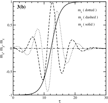
Figure 3: Precessional reversal of the magnetic moment for $\eta=2$ and $a=1$. Fig. 3(a) shows the locus (dotted curve) of ${\bf m}$ and Fig. 3(b) is for $m_{i}(\tau)$ vs. $\tau$. The initial direction of ${\bf m}$ is given by $\theta_{0}=\pi/1.01$ and $\phi_{0}=\pi/4$. Thin circles define a uni-sphere.

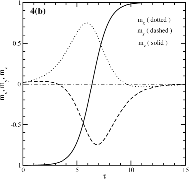
Figure 4: Plain reversal of the magnetic moment for $\eta=0.5$ and $a=1$. Fig. 4(a) shows the locus (dotted curve) of ${\bf m}$ and Fig. 4(b) is for $m_{i}(\tau)$ vs. $\tau$. The initial direction of ${\bf m}$ is the same as in Fig. 3. Note that there are no oscillations in $m_{x}$ and $m_{y}$. Thin circles define a uni-sphere.

Figure 5: Locus of ${\bf m}$ for $\eta=0.5$ (thick dotted curve)and $\eta=4$ (dotted curve). In Fig. 5(a), $a=0.5$ while $a=2$ in Fig. 5(b). Regardless of $a$, no precession occurs when $\eta=0.25$. Thin circles define a uni-sphere.

One can define the relaxation time $\tau_{0}$ of the reversal as an elapsed time during the reversal between $\theta\simeq\pi$ and $\theta\simeq 0$. When $m_{z}\simeq 1$, we can parametrize $\ln\left[1-m_{z}(\tau)\right]=c_{1}-c_{2}\tau/\tau_{0}$, where $c_{1}\approx 8.9$ and $c_{2}\approx 13.6$. We found these values are independent of $\eta$ and $a$. For given $\eta$ and $a$, we can determine $\tau_{0}$ by comparing numerical results with $c_{1}-c_{2}\tau/\tau_{0}$. For example, $\tau_{0}\simeq 7.9$ for $\eta=0.9$ and $a=1$. In general, the smaller $a$ (or $l$) is, the longer $\tau_{0}$ is for a given $\eta$. This can be understood because the wave function $|\psi_{tr}\rangle$ decays faster if $l$ is shorter so that the spin transfer is relatively less effective and, thus, it takes a longer time to reverse ${\bf m}$. In Fig. 6, we plot $m_{z}$ vs. $\tau$ for $\eta=4$ (main frame) and for $\eta=0.25$ (inset) with $a=0.5$ (solid) $1$ (dashed), and $2$ (dotted curve). In this figure, we can see the relation between $a$ and $\tau_{0}$ mentioned above. For $\eta\geq 1$, as $a$ increases, weak precession occurs because $\tau_{0}$ decreases as seen in the main frame of Fig. 6; in other words, ${\bf m}$ does not have enough time to precess strongly. We can also see such a behavior in Fig. 5 comparing $a=0.5$ and $a=2$ for $\eta=4$.

We plot $\tau_{0}$ vs. $\eta$ in Fig. 7 for a given $a$. The relaxation time is evaluated using the parameterization: $\ln\left[1-m_{z}(\tau)\right]=c_{1}-c_{2}\tau/\tau_{0}$. In the main frame, $a=1$ while in the inset $a=2$. At $\tau=\tau_{0}$, $m_{z}(\tau_{0})\simeq 0.99$ for all plots. Interestingly, $\tau_{0}$ is minimum at $\eta\simeq 1$. Therefore it is possible to estimate the microscopic coupling parameter $J_{H}$ between an incoming spin and a magnetic moment by measuring $\tau_{0}(\eta)$, because $\tau_{0}$ has a minimum for a given mean free path.

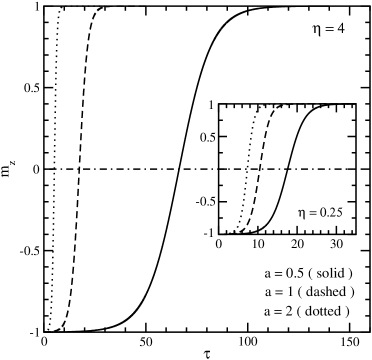
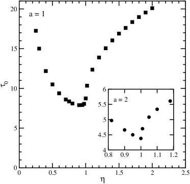
Figure 6: $m_{z}$ as a function of $\tau$. In the main frame, $\eta=4$ while in the inset $\eta=0.25$ with $a=0.5$ (solid) $1$ (dashed), and $2$ (dotted curve).

Figure 7: The relaxation time $\tau_{0}$ vs. $\eta$. In the main frame, $a=1$ while in the inset $a=2$. $\tau_{0}$ has a minimum value at $\eta\simeq 1$.

IV discussion and summary

In this section we would like to discuss the adiabatic approximation, which we tacitly used to study the dynamics of a magnetic moment. First we summarize the procedure we followed. We calculated ${\langle{\bf s}\rangle}$ using $|\psi(x)\rangle$; namely, $\langle{\bf s}\rangle=(1/2)\langle\psi(x)|{\bf\sigma}|\psi(x)\rangle$ for $x>0$ to solve ${d{\bf M}}/{dt}=2\gamma_{0}J_{H}\left({\bf M}\times{\langle{\bf s}\rangle}\right)$. Here we mention that $|\psi(x>0)\rangle$ is obtained by considering the Hamiltonian at a given time $t$ following Ref.berger Since the incoming wave function $|\psi_{in}\rangle\sim|+\rangle$ is not an eigenstate of the Hamiltonian for $x>0$, we have a linear combination of $|+\rangle$ and $|-\rangle$ for $|\psi(x>0)\rangle$ and $|\psi(x<0)\rangle$. The matching conditions of wave functions at $x=0$ allow us to express the coefficients of the combination for $|\psi(x>0)\rangle$ in terms of ${\bf M}(t)$ (see Eqs. (9) and (10)). Now ${\langle{\bf s}\rangle}$ is a function of ${\bf M}(t)$, and the time dependence of ${\langle{\bf s}\rangle}$ is given exclusively by ${\bf M}(t)$. This means that the time evolution of the wave function for $x>0$ is not fully taken into account. In addition to the equation for ${d{\bf M}}/{dt}$, one can derive the time derivative of the spin operator using $d{\bf s}/dt=i\left[H,{\bf s}\right]$:

$$\frac{d{\bf s}}{dt}+\nabla\cdot{\cal J}=2J_{H}\left({\bf s}\times{\bf M}\right)\;,$$ (16)

where ${\cal J}$ is the spin-current tensor. It is obvious that when we calculate an expectation value of ${\bf s}$ in Eq.(16) we need to use $|\psi(x,t)\rangle$; $\langle{\bf s}\rangle_{t}=(1/2)\langle\psi(x,t)|\sigma|\psi(x,t)\rangle$, where $|\psi(x,t)\rangle$ is obtained from $i\frac{d}{dt}|\psi(x,t)\rangle=H|\psi(x,t)\rangle$. Rigorously speaking, one has to solve the two coupled equations for ${\bf M}$ and ${\bf s}$ using $|\psi(x,t)\rangle$ to calculate the expectation value of ${\bf s}$ and $\nabla\cdot{\cal J}$. However, if we compare Eq. (5) or (14) with Eq. (16), we see that Eq. (14) has a factor $1/S_{local}$ while Eq. (16) does not. This means that if we treat the magnetic moment semiclassically, i.e. $S_{local}\gg 1$, then the time scale of Eq. (14) is much longer than that of Eq. (16). Therefore, the adiabatic approximation is applicable to our analysis.

In summary, we have studied the effect of an incoming spin-polarized current on a local magnetic moment in a magnetic thin film. We found that the spin torque occurs only when the incoming spin changes as a function of time inside of the magnetic film. If the incoming spin remains parallel to its initial direction, no spin torque takes place. This implies that some modifications are necessary in a phenomenological model where the coefficient of the spin torque term is a constant. Moreover, the coefficient is determined by dynamics instead of geometrical details. The magnetization reversal can be precessional as well as non-precessional depending on the incoming energy of electrons in the spin-polarized current. If the incoming energy is greater than the interaction energy $(J_{H}M_{0})$, the magnetization precesses while reversing its direction. For the incoming energy smaller than $J_{H}M_{0}$, the magnetization reversal is non-precessional. We also found that the relaxation time associated with the reversal depends on the incoming energy for a given mean free path. Our numerical calculations imply the coupling between an incoming spin and a magnetic moment $J_{H}$ can be estimated by measuring the relaxation time.

References

(1) See, for example, Spin Dynamics
in Confined magnetic Structure I edited by B. Hillebrands and
K. Ounadjela (Springer-Verlag, 2002).