Bosonizing one-dimensional cold atomic gases

Abstract

We present results for the long-distance asymptotics of correlation functions of mesoscopic one-dimensional systems with periodic and open (Dirichlet) boundary conditions, as well as at finite temperature in the thermodynamic limit. The results are obtained using Haldane’s harmonic-fluid approach (also known as “bosonization”), and are valid for both bosons and fermions, in weakly and strongly interacting regimes. The harmonic-fluid approach and the method to compute the correlation functions using conformal transformations are explained in great detail. As an application relevant to one-dimensional systems of cold atomic gases, we consider the model of bosons interacting with a zero-range potential. The Luttinger-liquid parameters are obtained from the exact solution by solving the Bethe-ansatz equations in finite-size systems. The range of applicability of the approach is discussed, and the prefactor of the one-body density matrix of bosons is fixed by finding an appropriate parametrization of the weak-coupling result. The formula thus obtained is shown to be accurate, when compared with recent diffusion Monte Carlo calculations, within less than $10\%$. The experimental implications of these results for Bragg scattering experiments at low and high momenta are also discussed.

I Introduction

A number of recent experiments Gorlitz01 ; Wada01 ; Schreck01 ; Hansel01 ; Greiner01 have demonstrated the possibility of confining atoms to one dimension. This possibility has produced an outburst of theoretical activity over the last years Olshanii98 ; Petrov00 ; Andersen02 ; Girardeau01 ; Dunjko01 ; Carusotto03 ; Papenbrock03 ; Gangardt03 ; Recati03 ; Buchler03 ; Cazalilla02 ; Luxat03 ; Olshanii02 ; Mora02 ; Giorgini02 ; Xianlong03 ; Cazalilla03 in the field of cold atoms. One important focus of these studies has been on the correlation properties of these new one-dimensional systems, with the goal of providing means to characterize them experimentally.

Although one-dimensional models have been the favorite toy of mathematical physicists during the last century, they only became experimentally relevant in the late 1960’s and 1970’s in connection with a number of solid-state materials exhibiting very anisotropic magnetic and electronic properties. Later, in the 1980’s and 1990’s, advances in chemical synthesis and nanotechnology made it possible to manufacture materials and devices where electrons are mainly confined to move along one or a few conduction channels. The latest experimental developments in the field of cold atoms, however, have several distinct features. First of all, the constituent particles are not electrons but bosonic atoms (although in the future fermionic atoms can also become available). Second, the “fundamental” interaction is no longer of Coulombic type but a short range potential. Furthermore, in the case of dilute atomic vapors confined in magnetic and/or optical traps, the degree of controllability over parameters such density and interaction strength seems unprecedented. This allows, in principle, to exhaustively explore phase diagrams, or to cleanly realize quantum-phase transitions, which so far are considered as theorists’ extreme idealizations of “dirty” solid-state phenomena.

The only a priori limitation offered by the atomic systems, at least from the point of view of a condensed matter theorist, seems to be their mesoscopic, rather than macroscopic, size. However, numerical calculations over the past decades (e.g. Affleck01 ; DMRG ) have taught us that many of the behaviors predicted for the thermodynamic limit, already manifest themselves at the mesoscopic scale, even when the system under study consists of just a few tens of particles. Furthermore, the study of mesoscopic systems is also a brach of modern condensed-matter physics as phenomena taking place at the mesoscopic scale have an undeniable interest. Thus the main of motivation of this paper is to present a set of tools that can be used to analyze the properties of these mesoscopic one-dimensional (1D) systems. Our main theoretical tool in this analysis is the harmonic-fluid approach, which is nothing but the relevant quantum hydrodynamics for 1D systems.

The harmonic-fluid approach has a long history Tomonaga50 ; LiebMattis65 ; Luther74 ; EfetovLarkin75 , which in some respects culminated with the work of Haldane Haldane81b ; Haldane81a . He realized that many one-dimensional models exhibiting gapless excitations with a linear spectrum can be described within the same framework. This framework defined a universality class of systems that Haldane termed “Luttinger liquids”. The name stems from an analogy with higher dimensional fermionic systems, where the equivalent role is played by the (universality class of) Fermi liquids. In the context of one-dimensional Fermi systems this approach has a second, more frequently used, name: “bosonization”. This refers to the fact that the method shows how to describe the low-energy degrees of freedom of the fermions in terms of a bosonic field which obeys a relativistic wave equation. However, differently from the Fermi liquids, the class of Luttinger liquids also includes one-dimensional interacting boson systems. As we shall discuss below, this has to do with absence of a well-defined concept of statistics in 1D. As a consequence, boson systems can display fermion-like properties and vice-versa. One well-known example in the field of cold atoms is the behavior of the Tonks gas, where the bosons interact so strongly that they effectively behave as free fermions.

Besides blurring the line that separates bosons from fermions, confinement to one-dimension has another peculiarity that is worth discussing. Being all transverse degrees of freedom frozen, fluctuations can only propagate longitudinally. This implies that their effect is enormously enhanced. As a consequence, no long-range order that breaks a continuous symmetry can exist in the thermodynamic limit, even at zero temperature.

The harmonic-fluid approach has several advantages over other approaches that are commonly employed to study the low-temperature behavior of 1D systems. First of all, it is not a mean field theory, and therefore does not break any symmetry. Furthermore, it can treat bosons and fermions on equal footing, their difference being manifested by the different structure of the correlation functions that describe them. It can also deal with strongly and weakly interacting systems at the same time since the low-energy physics parametrized by three phenomenological parameters (the particle density and two stiffnesses). These parameters are related to measurable properties of the system, which makes the approach conceptually simple. Nonetheless, one has to be aware of its limitations, which essentially are related to its “effective field-theory” character. Therefore, the description is a low-energy one, it comes with a built-in cut-off, and it is unable to describe the high-energy structure or any model-specific (i.e. non-universal) features. In some situations, when the interactions are strong, relating some of the phenomenological parameters to microscopic ones can be difficult. But in many such cases one can rely on an exact (i.e. Bethe-ansatz) solution to extract them. This will be illustrated here for the case of bosons interacting via a zero-range potential Lieb63a ; Lieb63b . We will thus be able to show that many of the results obtained in the weakly interacting limit from the Bogoliubov-Popov Popov ; Popov80 approach and its modifications Andersen02 ; Mora02 can be recovered and understood within the harmonic-fluid approach. We shall also present result for the correlation functions of a number of “toy models” of 1D mesoscopic systems, such like a ring (i.e. a small system with periodic boundary conditions) and a box (a system with open boundary conditions). Besides being analytically tractable, these models are important when comparing with numerical simulations using Monte Carlo methods Giorgini02 ; Carusotto03 ; Troyer02 , where periodic boundary conditions are used, or the density-matrix renormalization-group (DMRG) DMRG ; Kollath03 , for which open boundary conditions are best suited. Furthermore, in recent times, traps other than harmonic have become available Hansel01 ; Sauer01 , which also makes relevant the study of these geometries.

There already exist some studies of the correlation functions in finite-size systems in the literature, but they have mostly focused on fermionic or spin correlations Fabrizio95 ; Eggert96 ; Wang96 ; Affleck01 . The present approach allows to obtain the corrrelation functions for both bosons and fermions at the same time, and automatically includes all higher-harmonics, which have been omitted in previous treatments. Besides presenting in full detail the generalization of the harmonic-fluid approach to the box case, in this paper we also address how to fix the prefactor of the one-body density matrix for bosons interacting with a zero-range potential (henceforth referred to as “delta-inteacting bosons”). We find that, when properly parametrized, the result obtained by Popov in the weakly interacting limit Popov80 is accurate even in the strong coupling limit. This is demonstrated by comparing with exact results Lenard72 and recent diffusion Monte Carlo data Giorgini02 .

The organization of this paper is as follows: In the following section, we shall review the harmonic-fluid approach following Ref. Haldane81b, . In this section we also present its generalization to open boundary conditions. In Sect. III, results for different correlation functions in the box and the ring, as well as finite-temperature expressions in the thermodynamic limit, are presented. We consider both bosons and spinless (i.e. spin-polarized) fermions. Sect. IV specializes the discussion to a system of delta-interacting bosons. This model is relevant for bosonic atoms confined to a one-dimensional channel. We show how the parameters needed for the low-energy description can be extracted from the exact (Bethe-ansatz) solution, and discuss how to fix the prefactor of the one-body density matrix. Some experimental consequences of the correlation functions obtained within the harmonic-fluid approach are presented in this section. In particular, the line-shape of the momentum distribution at finite temperature is analyzed as the parameters of the system are varied. In Sect. V, we discuss the asymptotic structure of the wave-function of a bosonic Luttinger liquid, and obtain an expression for a system with open boundary conditions Finally, the appendices contain a proof of a commutation relation used in the main text, an alternative “derivation” of the low-energy Hamiltonian using the path integral formalism, as well as a detailed description of how to compute correlation functions using conformal field theory methods. Some of the results of this work have been briefly reported in Ref. Cazalilla02, .

II The harmonic-fluid approach

In this section we are going to review the harmonic-fluid approach in operator language, following the original work of Haldane Haldane81b . Some of the results of this section can be also obtained using a coherent-state path integral formulation (see Appendix B).

II.1 Haldane’s construction

The discussion in this subsection will be independent of boundary conditions, but we shall assume the system to have a finite size $L$. For the most part, the notation is similar to that of Haldane in Ref. Haldane81b, . However, we deviate from it in a number of places, sometimes to agree with more recent conventions. We shall work in second quantization most of the time. This means that a system of bosons is described using field operators which obey $[\Psi(x),\Psi^{\dagger}(x^{\prime})]=\delta(x-x^{\prime})$, and commute otherwise; $\rho(x)=\Psi^{\dagger}(x)\Psi(x)$ is the density operator. The mean ground state density, $\rho_{0}$, is fixed either by the chemical potential, $\mu$, such that $\rho_{0}=\rho_{0}(\mu)$ (grand canonical ensemble), or by the total particle number in the ground state, $N_{0}$, such that $\rho_{0}=N_{0}/L$ (canonical ensemble). Note that the discussion that follows applies to uniform systems, the necessary modifications needed to deal with a non-uniform (but slowly varying) ground state density are discussed in Sect. II.5.

As pointed out in the introduction, the effect of long wave-length thermal and quantum fluctuations is enhanced by reduced dimensionality. In order to derive a low-temperature description, we need to identify a set of variables that describe the low-energy fluctuations of the system. For a bosonic system these variables are the density and the phase. At low temperatures, density and phase fluctuations are locally small in the sense to be defined below. To give a proper definition of these variables, we need to introduce the phase-density representation of the bosonic field operator:

$$\Psi^{\dagger}(x)=\sqrt{\rho(x)}\>e^{-i\phi(x)}.$$ (1)

Consistently with the bosonic commutation relations $\left[\Psi(x),\Psi^{{\dagger}}(x)\right]=\delta(x-x^{\prime})$, phase and density operators obey

$$e^{i\phi(x^{\prime})}\rho(x)e^{-i\phi(x^{\prime})}-\rho(x)=\delta(x-x^{\prime}).$$ (2)

A convenient way of describing the long wave-length density and phase fluctuations is to split $\rho(x)=\rho_{<}(x)+\rho_{>}(x)$ and $\phi(x)=\phi_{<}(x)+\phi_{>}(x)$, where the $\rho_{<}(x)$ and $\phi_{<}(x)$ refer to the “slow” parts (i.e. coarse-grained over distances $\gg\rho^{-1}_{0}$) of the operators, whereas $\rho_{>}(x)$ and $\phi_{>}(x)$ refer to the “fast” or short-wave length parts (see Appendix B for a more careful definition). In the following we focus on the slow parts, and below, when there is not risk of confusion, we will denote as $\phi(x)$ the slow part of the phase operator (i.e. $\phi_{<}(x)$). Furthermore, since the density fluctuates at low temperatures about the ground state value, $\rho_{0}$, it is convenient to introduce the operator $\Pi(x)$, defined by $\rho_{<}(x)=\rho_{0}+\Pi(x)$.

Figure 1: Low-energy excitations in a Tonks ($=$ free Fermi) gas. The continuous arrow represents excitations about $+p_{F}$ (symmetrically, about $-p_{F}$) with momenta $q\approx 0$. The dashed arrow represents low-energy excitations carrying momenta $q\approx\pm 2p_{F}=\pm 2\pi\rho_{0}$.

We shall first consider the phase fluctuations. In Appendix A we show that the slow parts $\phi(x)$ and $\Pi(x)$ are canonically conjugated fields, i.e.

$$[\Pi(x),\phi(x^{\prime})]=i\>\delta(x-x^{\prime}).$$ (3)

It is worth pointing out that this commutation relation holds, for the slow parts of the density and phase, in arbitrary dimensions. However, since in 1D fluctuations are constrained to propagate on a line, this causes the aforementioned enhancement of their effect. This makes it impossible, in the thermodynamic limit, to define of an order parameter. Thus we expect that $\langle e^{i\phi(x)}\rangle=0$ in 1D, in contrast with the situation for $d>1$, where this operator can acquire a non-zero expectation value (i.e. there can be off-diagonal long-range order). Indeed, in one dimension $\langle e^{i\phi(x)}\rangle=0$ also in finite-size systems (see appendices C and  D).

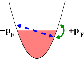
We next consider long wave-length fluctuations of the density, which have been parametrized as $\rho_{0}+\Pi(x)$. $\Pi(x)$ describes locally small fluctuations of wave-length $\gg\rho^{-1}_{0}$. However, this does not suffice to describe all possible low-energy density fluctuations. It is thus necessary to distinguish between “low-energy” and long “wave-length”; There can be low-energy density fluctuations with wave-length $\sim\rho^{-1}_{0}$ or shorter. To see this in a non-trivial case, it suffices to consider the case of the impenetrable-boson (Tonks) gas. It is known Girardeau60 ; Lieb63b that the excitations of such a system are those of a free fermi gas of the same density. In a Fermi gas the momentum of the fastest particle (the Fermi momentum) is related to the density by the formula $p_{F}=\pi\rho_{0}$. There are two Fermi points (see Fig. 1), corresponding to $p=\pm p_{F}$. The low-energy and long wave-length density fluctuations of this system are the small momentum particle-hole excitations around each one of the Fermi points. However, a fermion can also be excited with very low energy from one Fermi point to the other, thus producing a density fluctuation that oscillates as $\cos 2p_{F}x=\cos 2\pi\rho_{0}x$. The long wave-length density fluctuations described by $\Pi(x)$ lead to small changes in the local Fermi momentum: $p_{F}(x)=p_{F}+\pi\Pi(x)$. This affects shorter wave-length density fluctuations, which now oscillate as $\cos 2\int^{x}dx^{\prime}p_{F}(x^{\prime})=\cos 2\Theta(x)$, where we have introduced the auxiliary field $\Theta(x)$, related to $\Pi(x)$ by means of the following expression EfetovLarkin75 ; Haldane81b :

$$\frac{1}{\pi}\partial_{x}\Theta(x)=\rho_{0}+\Pi(x).$$ (4)

Note that the integral on the left hand-side of (4) from $x=0$ to $x=L$ must be equal to total particle number operator $N$, namely

$$\Theta(L)-\Theta(0)=\pi N.$$ (5)

Figure 2: Typical configuration of $\Theta(x)$. Its value changes by $\pi$ every time $x$ surpasses the location of a particle. Note that $\Theta(x)$ is a slowly varying field.

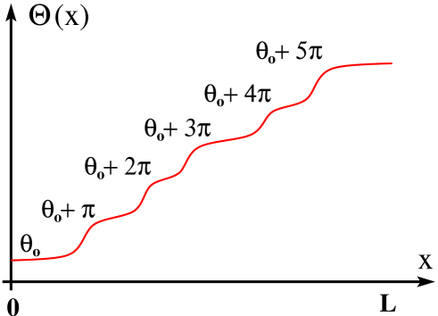
This is an important topological property of $\Theta(x)$. It tells us that on a global scale the changes in $\Theta(x)$ are related to changes in the total particle number. Hence, the configurations of $\Theta(x)$ can be regarded as functions that increase monotonically from $x=0$ to $x=L$ (see Fig. 2). Thus it is tempting to associate the location of particles with the points where $\Theta(x)$ equals an integer multiple of $\pi$. Physically this amounts to trading discrete particles by solitons or kinks in $\Theta(x)$ (see Fig. 2). The construction of a low-energy projection of the full density operator, $\rho(x)$, which reflects the discrete nature of the particles and therefore can describe the shorter wave-length low-energy fluctuations follows from this idea Haldane81b . First one sets:

$$\rho(x)=\partial_{x}\Theta(x)\sum_{n=-\infty}^{+\infty}\delta(\Theta(x)-n\pi),$$ (6)

which in the particle-soliton sense is equivalent to the first quantized form of the density operator, $\rho(x)=\sum_{i=1}^{N}\delta(x-x_{i})$ provided that $x_{i}$ is interpreted as the position operator of the particle-soliton and one uses $\delta[f(x)]=\delta(x-x_{0})/|f^{\prime}(x_{0})|$, where $f(x_{0})=0$. The previous expression can be rewritten in a more useful way with the help of Poisson’s summation formula:

$$\sum_{n=-\infty}^{+\infty}f(n)=\sum_{m=-\infty}^{+\infty}\,\int_{-\infty}^{+\infty}dz\,f(z)\>e^{2m\pi iz},$$ (7)

which yields:

$$\rho(x)=\frac{1}{\pi}\partial_{x}\Theta(x)\>\sum_{m=-\infty}^{+\infty}e^{2mi\Theta(x)}=\left[\rho_{0}+\Pi(x)\right]\>\sum_{m=-\infty}^{+\infty}e^{2mi\Theta(x)}.$$ (8)

This is the sought representation of the density operator. The $m=0$ term is precisely $\rho_{0}+\Pi(x)$, and describes the long wave-length fluctuations (i.e. those with momenta $|q|\ll\rho_{0}$), the $m=\pm 1$ terms describe fluctuations with $q\approx\pm 2\pi\rho_{0}$, while $m=\pm 2$ those with $q\approx\pm 4\pi\rho_{0}$, etc. (see Fig. 5).

We next take up the construction of the boson field operator $\Psi^{\dagger}(x)$ in terms of $\Theta(x)$ and $\phi(x)$. According to Eq. (1), this requires finding a representation for the square root of the density operator, Eq.(6). At this point it is useful to recall Fermi’s trick: $[\delta(\theta)]^{2}=A\>\delta(\theta)$, where the constant $A$ depends on the particular way the Dirac delta function is defined. Extracting the square root yields $\sqrt{\delta(\theta)}=A^{-1/2}\>\delta(\theta)$. Thus, using Poisson’s formula (7) and multiplying by $e^{-i\phi(x)}$ from the right, one arrives atHaldane81b :

$$\Psi^{\dagger}(x)\sim\left[\rho_{0}+\Pi(x)\right]^{\frac{1}{2}}\sum_{m=-\infty}^{+\infty}e^{2mi\Theta(x)}e^{-i\phi(x)}.$$ (9)

The symbol $\sim$ means that the field operator is given by the expression on the right up to a prefactor. This prefactor is not determined independently of the way we choose to exclude the high-energy fluctuations (i.e. the fast modes) from the low-temperature description. This is usually done using a cut-off in real or momentum space, and different cut-off schemes lead to different prefactors.

Figure 3: Effect on the string operator $e^{i\Theta(x)}$ of the creation of a particle at two different points $x_{1}$ (a) and $x_{2}$ (b). When a particle is created (or removed) at $x_{1}$, the string operator at $x_{2}<x_{1}$ is not affected (a). However, when the particle is created (or removed) at $x_{2}$ the value of the string at $x_{1}$ picks up an extra factor of $-1$. Since the operators $\Psi^{\dagger}_{F}(x)$ contain only odd powers of $e^{i\Theta(x)}$, they are sensitive to these changes, which implies that they anti-commute.

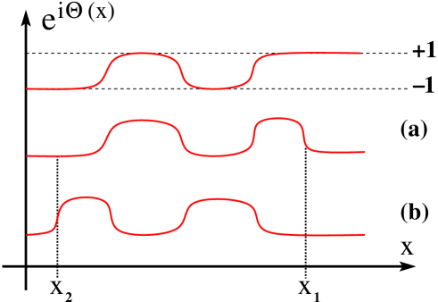
The construction of a fermionic (i.e. anti-commuting) field operator is also possible. One only needs to realize that, since $\Theta(x)$ jumps by $\pi$ every time a particle is surpassed (Fig. 3), the string operator $e^{i\Theta(x)}$ alternates between $+1$ and $-1$ (see Fig. 3). This implies that

$$\Psi^{\dagger}_{F}(x)=\Psi^{\dagger}(x)\>e^{i\Theta(x)}\sim\left[\rho_{0}+\Pi(x)\right]^{\frac{1}{2}}\sum_{m=-\infty}^{+\infty}e^{(2m+1)i\Theta(x)}\>e^{-i\phi(x)}$$ (10)

anti-commutes at different positions. To see this, consider the product $\Psi^{\dagger}_{F}(x_{2})\Psi^{\dagger}_{F}(x_{1})$ assuming that $x_{1}>x_{2}$, for instance. Since the operator $\Psi^{\dagger}_{F}(x_{1})$ acts first by creating a particle at $x_{1}$, it does not have any effect on the string operator at $x_{2}<x_{1}$ (see Fig. 3, case (a)). On the other hand, if we instead consider $\Psi^{\dagger}_{F}(x_{1})\Psi^{\dagger}_{F}(x_{2})$ ($x_{1}>x_{2}$), the operator $\Psi^{\dagger}_{F}(x_{2})$ acts first, thus creating at $x_{2}<x_{1}$. Therefore, the string $e^{i\Theta(x_{1})}$ of the second field operator picks up an extra minus sign (see Fig. 3, case (b)) relative to the case where a particle is created at $x_{1}$ first. Thus the operator defined by (10) anti-commutes at different locations, and therefore describes fermions instead of bosons. The same conclusion can be reached for a product of two annihilation (or one creation and one annihilation) operators at different points .

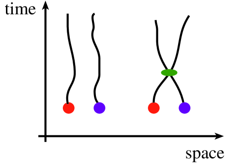
The explicit construction of the low-energy representations of commuting (i.e. bosonic) and anti-commuting (i.e. fermionic) fields shows how this approach treats bosons and fermions on equal footing. On physical grounds, the fact that in 1D transforming bosons into fermions is possible is not a surprise. The reason Haldane81b is that when one tries to exchange two interacting particles (or elementary excitations) in 1D they must necessarily collide, and therefore the statistical phase cannot be separated from the phase shift associated with the collision (see Fig. 4).

Figure 4: When two particles are exchanged in one-dimension to test their statistics, they cannot avoid collision. Thus the statistical phase and the scattering phase shift cannot be separated.

II.2 Low-energy effective Hamiltonian and momentum operators

So far we have considered the kinematics of the low-energy description of a 1D quantum fluid. In other words, we have introduced the variables that describe low-temperature states of the system and found their relationship to density and field operators. The next step is to consider the dynamics, that is, the Hamiltonian. The starting point for our considerations is the following Hamiltonian for bosons interacting via a general two-body potential, $v(x)$ :

$$H=\frac{\hbar^{2}}{2M}\int_{0}^{L}dx\>\partial_{x}\Psi^{\dagger}(x)\partial_{x}\Psi(x)+\frac{1}{2}\int_{0}^{L}dx\;dx^{\prime}\,v(x-x^{\prime})\rho(x)\rho(x^{\prime}).$$ (11)

Before proceeding any further, a number of comments are in order: The above Hamiltonian is assumed to describe the situation where all particles lie in the lowest level of a transverse confining potential. This happens when the chemical potential, $\mu$, is smalller than the transverse confinement energy, $\hbar\omega_{\perp}$. Regarding the longitudinal confinement, we will assume in the following that it is either absent (case of periodic boundary conditions) or that it can be approximated by two infinite barriers placed at $x=0$ and $x=L$ (case of open boundary conditions). The effect of a smooth potential in the longitudinal direction will be discussed in Sect. II.5. By restricting ourselves to the lowest transverse level, we assume the system to be effectively one-dimensional. If $u_{0}^{\perp}(y,z)$ denotes the lowest transverse orbital, the three dimensional boson field operator can be written as $\Psi^{{\dagger}}_{3d}({\bf r})=\Psi^{{\dagger}}(x)\>u_{0}^{\perp}(y,z)+\tilde{\Psi}^{{\dagger}}({\bf r})$, where $\tilde{\Psi}^{{\dagger}}({\bf r})$ describes bosons in the higher energy transverse levels. At low temperatures (i.e. $T<\mu<\hbar\omega_{\perp}$), only virtual transitions to higher transverse levels are permitted, which lead to a renormalization of the interaction potential $v(x)$ (see e.g. Ref. Olshanii98, )

To obtain the low-energy effective Hamiltonian we use the operator identities derived in the previous section keeping only the leading terms, which are quadratic in the gradients of the slowly varying fields $\Theta(x)$ and $\phi(x)$ (alternatively, one can linearize the equations of motion for the density and the phase-gradient in terms of the gradients $\phi$ and $\Theta$). The result can be generally written as

$$H_{\rm eff}=\frac{\hbar}{2\pi}\int_{0}^{L}dx\>\left[v_{J}\left(\partial_{x}\phi(x)\right)^{2}+v_{N}\>\left(\partial_{x}\Theta(x)-\pi\rho_{0}\right)^{2}\right].$$ (12)

The history of this Hamiltonian goes back to the pioneering work of Tomonaga Tomonaga50 on one-dimensional electron gases. He wrote it in a very different way, but as we shall see in the following sections, both forms are essentially equivalent and describe the same collection of harmonic oscillators, whose quanta, the “phonons” correspond to low-energy density and phase fluctuations. The first application to a bosonic system was done by Efetov and Larkin EfetovLarkin75 , who considered a system of tightly bound electron pairs (the “BEC” limit of a 1D superconductor) and wrote $H_{\rm eff}$ in a form similar to Eq. (12). The form used here is due to Haldane Haldane81a ; Haldane81b who, building upon and extending the work of Tomonaga Tomonaga50 , Lieb and Mattis LiebMattis65 , Luther Luther74 , Efetov and Larkin EfetovLarkin75 ,… introduced the concept of (Tomonaga-) Luttinger liquid as a universality class of 1D systems with gapless, linearly-dispersing, excitations.

For an interaction whose range $R\gg\rho^{-1}_{0}$, one should replace the second term in $H_{\rm eff}$ by

$$\frac{1}{2\pi^{2}}\int_{0}^{L}dx\;dx^{\prime}\,v(x-x^{\prime})(\partial_{x}\Theta(x)-\pi\rho_{0})(\partial_{x^{\prime}}\Theta(x^{\prime})-\pi\rho_{0}).$$ (13)

However, provided that the Fourier transform of the interaction potential $v(q)=\int^{L}_{0}dx\,e^{-iqx}v(x)$ is not singular as $q\to 0$, Eq.(12) will hold at sufficiently low energies, and below we shall assume that this is indeed the case (a notable exception is the Coulomb interaction). The term proportional to $(\partial_{x}\Theta-\pi\rho_{0})^{2}$ in Eq. (12) thus corresponds to the interaction energy of the long wave-length density fluctuations. The density stiffness $v_{N}$ has dimensions of velocity. In the following subsection, it is shown that it is inversely proportional to the compressibility of the fluid. The phase stiffness $v_{J}$ has also velocity units and it is found to be proportional to the superfluid fraction. Therefore, both parameters must be regarded as phenomenological. They can be extracted from an exact solution of the microscopic model (when available), from numerical calculations or, ultimately, from experimental data, which still allows one to correlate the results from different experiments.

For many models on the continuum (i.e. those which do not require a lattice to be defined) the term proportional to $(\partial_{x}\phi)^{2}$ in Eq. (12) follows from the kinetic energy operator after using Eq. (9), i.e.

$$\frac{\hbar^{2}}{2M}\>\int_{0}^{L}dx\>\partial_{x}\Psi^{\dagger}(x)\partial_{x}\Psi(x)\approx\frac{\hbar^{2}\rho_{0}}{2M}\int_{0}^{L}dx\>\left(\partial_{x}\phi(x)\right)^{2}.$$ (14)

Hence $v_{J}=\hbar\pi\rho_{0}/m\equiv v_{F}$, where $v_{F}$, is the Fermi velocity of a gas of free spinless fermions of density $\rho_{0}$. As we show in the following subsection, this relationship between $v_{J}$ and $v_{F}$ is ensured by Galilean invariance, and will not hold if this symmetry is broken. This is generally the case of lattice models, such like a 1D system of bosons hopping in a sufficiently deep optical lattice

Another interesting operator is the total momentum, which can also be expressed in terms of $\Theta(x)$ and $\phi(x)$. The derivation is similar to that of the Hamiltonian, starting from the second quantized form,

$$P=\frac{\hbar}{2i}\int^{L}_{0}\left[\Psi^{\dagger}(x)\partial_{x}\Psi(x)-\partial_{x}\Psi^{\dagger}(x)\Psi(x)\right],$$ (15)

we keep the leading terms in the gradients of $\Theta(x)$ and $\phi(x)$, and obtain

$$P=\frac{\hbar}{\pi}\int^{L}_{0}\partial_{x}\Theta(x)\partial_{x}\phi(x).$$ (16)

We close this subsection with a remark about notation. It is customary in the literature on bosonization to work with the field

$$\theta(x)=\Theta(x)-\pi\rho_{0}x,$$ (17)

instead of $\Theta(x)$. Hence, $\Pi(x)=\partial_{x}\theta(x)/\pi$. It is also common to introduce the parameters $K=\sqrt{v_{J}/v_{N}}$ and $v_{s}=\sqrt{v_{N}v_{J}}$, such that

$$H_{\rm eff}=\frac{\hbar v_{s}}{2}\int_{0}^{L}dx\>\left[\frac{K}{\pi}\left(\partial_{x}\phi(x)\right)^{2}+\frac{\pi}{K}\>\left(\Pi(x)\right)^{2}\right]=\frac{\hbar v_{s}}{2\pi}\int_{0}^{L}dx\>\left[K\left(\partial_{x}\phi(x)\right)^{2}+\frac{1}{K}\>\left(\partial_{x}\theta(x)\right)^{2}\right]$$ (18)

As we shall see shortly, $v_{s}$ is the phase velocity of the low-energy excitations (sound waves). However, the dimensionless parameter $K$ is related to the strength of quantum fluctuations (see Appendix B).

II.3 Particles in a ring: periodic boundary conditions.

Our first task in this subsection will be to find appropriate mode expansions for the fields $\Theta(x)$ and $\phi(x)$, such that the Hamiltonian, Eq. (12), is diagonalized. Before doing it, we need to find out how to implement the boundary conditions in terms of these fields. Therefore, consider a system obeying periodic boundary conditions. As commonly introduced in the literature, this seems a mere mathematical convenience that simplifies the calculations before taking the thermodynamic limit. However, nowadays there exist experimental realizations of these BC’s. In the case of cold atoms one can think of a quantum degenerate atomic gas in a tight toroidal trap Sauer01 . Thus, if the boson field obeys $\Psi^{\dagger}(x+L)=\Psi^{\dagger}(x)$, then equations (5) and (8,9) imply that:

$$\Theta(x+L) = \Theta(x)+\pi N,$$ (19)

$$\phi(x+L) = \phi(x)+\pi J,$$ (20)

where $N$ is the particle-number operator, and $J$ is an operator whose eigenvalues are even integers so that $(-1)^{J}=+1$. These are very important topological properties of the phase and density fields. In particular, they imply that the system has states that can be labeled by the eigenvalues of $J$ and $N$. We show below that $N$ and $J$ are conserved quantities (i.e. they commute with $H_{\rm eff}$) and can be used to label topologically excited states of the system. In the case of $N$ this is not surprising because the microscopic Hamiltonian, Eq. (11), conserves the total particle number. However, we will see that $J$ is associated with the possibility of quantized persistent currents.

We next write down the mode expansions for $\Theta(x)$ and $\phi(x)$, which obey (19) and (20), as well as the commutation relation:

$$\left[\partial_{x}\Theta(x),\phi(x^{\prime})\right]=i\pi\delta(x-x^{\prime}).$$ (21)

The appropriate expressions read:

$$\Theta(x) = \theta_{0}+\frac{\pi x}{L}N+\frac{1}{2}\sum_{q\neq 0}\Big{|}\frac{2\pi K}{qL}\Big{|}^{\frac{1}{2}}e^{-a|q|/2}\big{[}e^{iqx}b(q)+e^{-iqx}b^{\dagger}(q)\big{]},$$ (22)

$$\phi(x) = \phi_{0}+\frac{\pi x}{L}J+\frac{1}{2}\sum_{q\neq 0}\Big{|}\frac{2\pi}{qLK}\Big{|}^{\frac{1}{2}}e^{-a|q|/2}{\rm sgn}(q)\big{[}e^{iqx}b(q)+e^{-iqx}b^{\dagger}(q)\big{]}.$$ (23)

The operators $b(q)$ and $b^{\dagger}(q)$ have the commutation relation:

$$[b(q),b^{\dagger}(q^{\prime})]=\delta_{q,q^{\prime}},$$ (24)

commuting otherwise. Momenta are quantized as $q=2\pi m/L$, where $m=0,\pm 1,\pm 2,\pm 3,\ldots$ The pairs $(N,\phi_{0})$ and $(J,\theta_{0})$ are conjugate action-angle variables which obey:

$$\left[N,e^{-i\phi_{0}}\right] = e^{-i\phi_{0}},$$ (25)

$$\left[J,e^{-i\theta_{0}}\right] = e^{-i\theta_{0}}$$ (26)

$$\left[J,N\right] = \left[\phi_{0},\theta_{0}\right]=0.$$ (27)

Figure 5: Typical low-energy excitation spectrum of a Luttinger liquid with periodic boundary conditions. The shaded area corresponds to the continuum of multi-particle-hole excitations. The Hamiltonian $H_{\rm eff}$, Eq. (28) describes the excitation spectrum for $q\approx\pi J\rho_{0}$, with $J=0,\pm 2,\pm 4,\ldots$. Near $q\approx 0$ the excitations are linearly dispersing phonons: $\omega(q)\simeq\hbar v_{s}|q|$ (i.e. superpositions of particle-hole excitations about the same Fermi point, see Fig. 1). For $q\sim\pi J\rho_{0}$, where $J=\pm 2,\pm 4,\ldots$, the excitations involve the creation of $J$ current quanta in the ring. For instance, $J=\pm 2$ correspond to the low-energy transitions between Fermi points shown in Fig. 2 (dashed arrow). For delta-interacting bosons, this picture holds in all regimes, and for the particle-hole spectrum agrees with the spectrum obtained from Bethe ansatz in Ref. CastroNeto94 .

Introducing the expressions (22) and (23) into Eq. (12), one obtains:

$$H_{\rm eff}=\sum_{q\neq 0}\hbar\omega(q)\>b^{\dagger}(q)b(q)+\frac{\hbar\pi v_{s}}{2LK}(N-N_{0})^{2}+\frac{\hbar\pi v_{s}K}{2L}J^{2}+{\rm const.},$$ (28)

where $\omega(q)=v_{s}|q|$ for $q\ll\rho^{-1}_{0}$. It now becomes clear that this Hamiltonian describes collective phonon-like excitations (sometimes called Tomonaga bosons Tomonaga50 ), which disperse linearly in the long wave-length limit $|q|\to 0$. This result is perhaps not striking if one deals with bosons because it is already obtained from Bogoliubov’s theory (although in 1D this theory is inconsistent in several respects, which can be cured only in the weakly interacting limit Popov ; Andersen02 ; Mora02 ). However, for interacting fermions it has striking consequences, because it means the absence of individual (i.e. particle-like) excitations in the low-energy spectrum, and the break-down of Fermi-liquid theory in 1D.

The expansions (22) and (23) diagonalize the momentum operator as well:

$$P=\frac{\hbar\pi}{L}NJ+\sum_{q\neq 0}\hbar q\,b^{\dagger}(q)b(q).$$ (29)

As $\Theta(x)$, $\phi(x)$, $H_{\rm eff}$ and $P$ describe long wave-length fluctuations, the momentum sums must be cut-off at a momentum $a^{-1}\lesssim\min\left\{R^{-1},q_{c}\right\}$. For short range interactions, $a^{-1}\lesssim q_{c}$; $q_{c}$ is then fixed by demanding that $\hbar v_{s}q_{c}=\mu$, i.e. it is an estimate of the momentum where the excitation spectrum deviates from the linear behavior.

From the previous expression for the Hamiltonian the (inverse) adiabatic compressibility at zero temperature can be obtained:

$$\kappa^{-1}_{S}=\rho_{0}^{2}\>\left(\frac{\partial\mu}{\partial\rho}\right)_{\rho=\rho_{0}}=\rho^{2}_{0}\>L\left[\frac{\partial^{2}E_{0}(N)}{\partial N^{2}}\right]_{N=N_{0}}=\hbar\pi v_{N}\rho^{2}_{0}=\frac{\hbar\pi v_{s}\rho^{2}_{0}}{K},$$ (30)

where $E_{0}(N)=\langle H\rangle_{N}$ is expectation value of the Hamiltonian, Eq. (28), taken over the ground state with $N$ particles; hence $v_{N}\propto\kappa_{S}^{-1}$. Using the previous expressions, we can also write:

$$v_{N}=\frac{1}{\pi\hbar}\,\left(\frac{\partial\mu}{\partial\rho}\right)_{\rho=\rho_{0}}=\frac{L}{\pi\hbar}\left[\frac{\partial^{2}E_{0}(N)}{\partial N^{2}}\right]_{N=N_{0}},$$ (31)

which will be useful in extracting the density stiffness from the Bethe-ansatz solution of the delta-interacting bosons in Sect. IV.1.

We next find the relationship between the phase stiffness, $v_{J}$, and the superfluid fraction, which we denote as $\rho_{s}$ below. To this purpose, we consider twisted boundary conditions instead of PBC’s:

$$\Psi^{{\dagger}}(x+L)=e^{-i\alpha}\Psi^{{\dagger}}(x).$$ (32)

Therefore, the phase field obeys the modified boundary conditions: $\phi(x+L)=\phi(x)+\pi J+\alpha$, such that $(-1)^{J}=+1$. This means that in Eq. (23) we have to shift $J\to J+\alpha/\pi$. As a result, the ground state energy and momentum are also shifted (recall that in the ground state $\langle N\rangle=N_{0}$ and $\langle J\rangle=0$):

$$\langle H_{\rm eff}\rangle_{\alpha\neq 0}-\langle H_{\rm eff}\rangle_{\alpha=0} = \frac{1}{2}\left(\frac{\hbar v_{J}}{\pi}\right)\left(\frac{\alpha}{L}\right)^{2}L,$$ (33)

$$\langle P\rangle_{\alpha\neq 0}-\langle P\rangle_{\alpha=0} = \hbar N_{0}\left(\frac{\alpha}{L}\right).$$ (34)

Thus we see that the system responds to the twist in the BC’s by drifting as whole with constant velocity $v_{sf}=(\langle P\rangle_{\alpha\neq 0}-\langle P\rangle_{\alpha=0})/(MN_{0})=\hbar\alpha/ML$. The superfluid fraction, $\rho_{s}$, can be obtained by regarding the shift in the ground state energy as the kinetic energy of the superfluid mass $M(\rho_{s}L)$:

$$\langle H_{\rm eff}\rangle_{\alpha\neq 0}-\langle H\rangle_{\alpha=0}=\frac{1}{2}M(\rho_{s}L)v^{2}_{sf}=\frac{\hbar^{2}\rho_{s}}{2M}\left(\frac{\alpha}{L}\right)^{2}L.$$ (35)

By comparing (33) and (35) we can identify

$$\frac{\hbar v_{J}}{\pi}=\frac{\hbar^{2}\rho_{s}}{M}.$$ (36)

Otherwise, in view of Eq. (33), we could have defined the phase stiffness in an analogous way to the density stiffness:

$$v_{J}=\frac{\pi L}{\hbar}\left(\frac{\partial^{2}E_{0}(\alpha)}{\partial\alpha^{2}}\right)_{\alpha=0},$$ (37)

where $E_{0}(\alpha)=\langle H\rangle_{\alpha\neq 0}$. Hence, $v_{J}$ is seen to be related to the response of the system to a phase twist just like $v_{N}$ is related to the response to a change in particle number. For charged particles the phase twist can be thought as the result of a magnetic flux that threads the ring Giamarchi95 .

We next specialize to Galilean invariant systems. As we have already anticipated in the previous section, for these systems $v_{J}=v_{F}=\hbar\pi\rho_{0}/M$, and therefore $\rho_{s}=\rho_{0}$. To prove this identity we perform a Galilean boost where the particle momenta are shifted: $p_{i}\to p^{\prime}_{i}=p_{i}+\hbar Q$. The Hamiltonian and momentum operators transform as:

$$H^{\prime} = H+\frac{\hbar Q}{M}P+N\frac{(\hbar Q)^{2}}{2M},$$ (38)

$$P^{\prime} = P+\hbar NQ.$$ (39)

Therefore, the ground state energy and momentum are shifted: $E^{\prime}_{0}-E_{0}=N(\hbar Q)^{2}/2M$, and $P^{\prime}_{0}=\hbar NQ$. Upon comparing the latter expression for $P$ with Eq. (29), we see that, to leading other, $Q=\pi J/L$. Hence, $E^{\prime}_{0}=E_{0}+(\hbar\pi)^{2}\rho_{0}J^{2}/(2L)$. However, from Eq. (28), the energy of the boosted state is $E^{\prime}_{0}=E_{0}+\hbar\pi v_{J}J^{2}/(2L)$. From these last two expressions it follows that $v_{J}=v_{F}$.

The previous analysis also allows to understand why no term involving the product $\partial_{x}\Theta(x)\partial_{x}\phi(x)$ appears in the low-energy Hamiltonian, Eq. (12). The reason is that this product is the momentum density (cf. Eq. (16)). Therefore, the presence of such a term in the Hamiltonian would indicate that we have not chosen the reference frame where the system is at rest. Thus one can get rid of it by a suitable Galilean transformation (cf. Eq. (38)).

We end this subsection with a discussion of the selection rules for the eigenvalues of $J$ and $N$. For bosons with PBC’s we have found the following selection rule: $(-1)^{J}=+1$, i.e. $J$ has eigenvalues that are even integers. However, obtaining the selection rule for fermions becomes somewhat messy using the above methods. To derive the selection rules for both bosons and fermions we recall here a construction due to Mironov and Zabrodin Mironov91 . The construction works directly with the many-particle wave function and therefore does not rely on the previous formalism. Consider a rigid translation of the system by a distance $a$, i.e.

$$e^{i\hat{P}a/\hbar}\Phi(x_{1},x_{2},\ldots,x_{N})=\Phi(x_{1}+a,x_{2},\ldots,x_{N}+a)$$ (40)

Let $\Phi$ be an eigenstate of the momentum operator $\hat{P}$ with eigenvalue $P$ and set $a=L/N=\rho^{-1}_{0}$, $x_{1}=x,x_{2}=x+a,\ldots,x_{N}=x+(N-1)a$. Thus,

$$e^{iPa/\hbar}\Phi(x,x+a,\ldots,x+(N-1)a)=\Phi(x+a,x+2a,\ldots,x)=(\pm 1)^{N-1}\Phi(x,x+a,\ldots,x+(N-1)a),$$ (41)

where the plus sign corresponds to bosons and the minus to fermions. The last equation follows from permuting the particle coordinates in the translated wave function to sort them in increasing order. The operation involves $N-1$ transpositions and therefore for fermions the signature of the permutation is $(-1)^{N-1}$. If we choose the wave function to be an eigenstate of $\hat{P}$ with $P=\hbar\pi JN/L$, we arrive at the selection rule:

$$(-1)^{J}=(\pm 1)^{N-1},$$ (42)

which reduces to $(-1)^{J}=+1$ for bosons, and to:

$$(-1)^{J}=-(-1)^{N}$$ (43)

for fermions. In the thermodynamic limit these selection rules are not very important because one can effectively treat $N$ and $J$ as having continuous eigenvalues. Furthermore, the terms in the Hamiltonian (28) proportional to $(N-N_{0})^{2}$ and $J^{2}$ are of order $L^{-1}$ and disappear as $L\to\infty$. However, for the mesoscopic systems which concern us here, the selection rules can be important in certain situations where one needs to keep track of finite-size effects and the discreteness of particles.

II.4 Particles in a box: open (Dirichlet) boundary conditions.

We now turn our attention to systems with open (Dirichlet) boundary conditions (OBC’s). In cold atom systems these conditions have been already experimentally realized (in an approximate way) Hansel01 using a microchip trap where the potential was shaped to a square-well with very high barriers, which can be approximated by perfectly reflecting walls. Less restrictively, one can assume that there are two points, $x=0$ and $x=L$, where current density vanishes, and this corresponds to the equilibrium state in the experiment of Ref. Wada01, , where ⁴He was confined in a long nanopore. To implement the latter BC’s, we first note that, from the continuity equation,

$$\partial_{t}\rho(x,t)+\partial_{x}j(x,t)=0,$$ (44)

and using that $\rho(x,t)\approx\partial_{x}\Theta(x)/\pi$, it follows that the current density $j(x,t)\approx-\partial_{t}\Theta(x,t)/\pi$. Hence, demanding that $j(x=0)=0$ amounts to $\partial_{t}\Theta(x=0,t)=0$, i.e. $\Theta(x=0,t)=\theta_{B}=$ const. However, what is often understood by open boundary conditions is something more restrictive than this: it is demanded that $\rho(x=0,t)=0$. This is achieved by the further requirement that $\theta_{B}\neq 0,\pm\pi,\pm 2\pi,\ldots$ In other words, $\Theta(x=0)$ must be pinned at real number that is not a multiple of $\pi$. To understand this, we need to go back to Eq. (6),

$$\rho(x)=\partial_{x}\Theta(x)\>\sum_{n=-\infty}^{+\infty}\delta(\Theta(x)-n\pi).$$ (45)

From this expression, one can see that $\rho(x=0)=0$ provided that $\Theta(x=0)=\theta_{B}\neq n\pi$, where $n$ is an integer. If $\rho(x=0)$ vanishes so does $\Psi^{{\dagger}}(x=0)\propto\sqrt{\rho(x=0)}$. What about the other end of a finite system (i.e. $x=L$)? The property

$$\left[\Theta(L)-\Theta(0)\right]=N\pi$$ (46)

also fixes $\Theta(L)=\Theta(0)+N\pi=\theta_{B}+N\pi$. Thus the boundary condition is automatically satisfied at $x=L$.

We now find the appropriate mode expansions for $\Theta(x)$ and $\phi(x)$. The requirements are the same as in the previous subsection, namely that the BC’s and the commutation relation of $\partial_{x}\Theta(x)$ and $\phi(x)$, Eq. (21), must be fulfilled for $0<x,x^{\prime}<L$. Thus we arrive at the following expressions (remember in what follows that $\theta_{B}$ is just a real number, not an operator):

$$\Theta(x) = \theta_{B}+\frac{\pi x}{L}N+i\sum_{q>0}\Big{(}\frac{\pi K}{qL}\Big{)}^{\frac{1}{2}}\>e^{-aq/2}\sin(qx)\big{[}b(q)-b^{\dagger}(q)\big{]},$$ (47)

$$\phi(x) = \phi_{0}+\sum_{q>0}\Big{(}\frac{\pi}{qLK}\Big{)}^{\frac{1}{2}}\>e^{-aq/2}\cos(qx)\big{[}b(q)+b^{\dagger}(q)\big{]}$$ (48)

where $a^{-1}\lesssim\min\left\{R^{-1},q_{c}=\mu/\hbar v_{s}\right\}$ and $q=m\pi/L$, with $m=1,2,3,\ldots$ Notice that in this case only one pair of action-angle operators is needed, $(N,\phi_{0})$. This is because in a box, as opposed to a ring, there cannot be persistent currents, and therefore $J$ is not a good quantum number.

The above mode expansions diagonalize the Hamiltonian and render it as follows:

$$H_{\rm eff}=\sum_{q>0}\hbar\omega(q)\>b^{\dagger}(q)b(q)+\frac{\hbar v_{s}\pi}{2LK}(N-N_{0})^{2},$$ (49)

with $\omega(q)=v_{s}q$ for $q\ll\rho_{0}$. The restriction $q>0$ means that $q$ cannot be interpreted as the momentum of the excitation but as its wave number. The sound waves in a system with OBC’s are standing waves and therefore do not carry momentum. Consistently, the momentum operator vanishes, i.e. $P=0$ .

II.5 Effect of a slowly varying confining potential

In most of current experimental setups cold atoms are confined in harmonic traps. In this section we are going to discuss how the harmonic-fluid approach must be modified when a smooth potential is applied in the longitudinal direction. We shall distinguish two situations. In the first we consider that the external potential is weak and show that much of what has been said above applies with small modifications. However, the harmonic potential does not belong to this class. In other words, it is not weak, but this does not mean that the harmonic-fluid approach cannot be adapted to this case. However, calculations are no longer analytically feasible (except in certain limits). Some results for harmonically trapped gases of bosons Gangardt03 and fermions Recati03 are already available in the literature, but since in general no explicit expressions for the correlation functions are available it is hard to extract much qualitative information from these results. In the Tonks limit, one can rely on the fermion-boson corresondence established by Girardeau Girardeau60 , which also allows to make a beautiful connection with the theory of random matrices in the gaussian unitary ensemble (GUE). This connection makes it possible to obtain the density profile Mehta , the form of the Friedel oscillations Kalisch02 as well as asymptotic forms for the one-body density matrix Forrester03 . It is also worth mentioning that for fermionic systems one can use constructive bosonization Haldane81a , and some analytical results can be thus obtained Xianlong03 . However, the problem with this approach is that the interactions between cold fermions do not have a simple form in the harmonic-oscillator basis. Therefore, it becomes hard to assess the effect of the different matrix elements on the low-energy physics.

Introducing an external potential amounts to adding to the Hamiltonian in Eq. (11) the following term

$$U_{\rm ext}=\int_{0}^{L}dx\>u_{\rm ext}(x)\rho(x).$$ (50)

Provided that $u_{\rm ext}(x)$ is weak (i.e. $|u_{\rm ext}(x)|\ll\mu$) and varies slowly over distances on the scale of $a$, it couples only to the slow part of the density operator, namely to $\partial_{x}\Theta(x)/\pi$. Hence,

$$H_{\rm eff}=\int_{0}^{L}dx\>\left\{\frac{\hbar v_{s}}{2\pi}\left[K\left(\partial_{x}\phi(x)\right)+\frac{1}{K}\left(\partial_{x}\Theta(x)-\pi\rho_{0}\right)^{2}\right]+\frac{u_{\rm ext}(x)}{\pi}\partial_{x}\Theta(x)\right\}.$$ (51)

Up to a constant, $H_{\rm eff}$ can be rewritten as:

$$H_{\rm eff}=\frac{\hbar v_{s}}{2\pi}\int_{0}^{L}dx\>\left[K\left(\partial_{x}\phi(x)\right)^{2}+\frac{1}{K}\left(\partial_{x}\Theta(x)-\pi\rho_{0}(x)\right)^{2}\right],$$ (52)

where $\rho_{0}(x)=\rho_{0}+\delta\rho_{0}(x)$, and

$$\delta\rho_{0}(x)=-\frac{K}{\hbar\pi v_{s}}u_{\rm ext}(x)=-\left(\frac{d\rho}{d\mu}\right)\>u_{\rm ext}(x).$$ (53)

The last expression follows from the relationship found in Eq. (30) between $K/\hbar\pi v_{s}$ and the compressibility. The result from linear response theory is thus recovered, since $u_{\rm ext}(x)$ enters the Hamiltonian as (minus) the chemical potential. In order to render the Hamiltonian to its form in the absence of $u_{\rm ext}$ it is convenient to shift

$$\tilde{\Theta}(x)=\Theta(x)-\pi\int_{0}^{x}dx^{\prime}\>\left[\rho_{0}(x^{\prime})-\rho_{0}\right],$$ (54)

such that the second term in Eq. (52) becomes:

$$\frac{\hbar v_{s}}{2\pi K}\int^{L}_{0}dx\left(\partial_{x}\tilde{\Theta}(x)-\pi\rho_{0}\right)^{2}.$$ (55)

The expansions in modes given in previous sections can now be used to diagonalize $H_{\rm eff}$ with $\tilde{\Theta}(x)$ playing the role of $\Theta(x)$. This leads to the same form for the spectrum, but the shift (54) must be taken into account when computing correlation functions. Thus, the density and field operators become:

$$\rho(x) = \left[\rho_{0}(x)+\frac{1}{\pi}\partial_{x}\tilde{\theta}(x)\right]\sum_{m=-\infty}^{+\infty}e^{2mi\pi\int_{0}^{x}dx^{\prime}\>\rho_{0}(x^{\prime})}\>e^{2mi\tilde{\theta}(x)},$$ (56)

$$\Psi^{{\dagger}}(x) \sim \left[\rho_{0}(x)+\frac{1}{\pi}\partial_{x}\tilde{\theta}(x)\right]^{1/2}\sum_{m=-\infty}^{+\infty}e^{2mi\pi\int_{0}^{x}dx^{\prime}\>\rho_{0}(x^{\prime})}\>e^{2mi\tilde{\theta}(x)}\>e^{-i\phi(x)},$$ (57)

$$\Psi^{{\dagger}}_{F}(x) \sim \left[\rho_{0}(x)+\frac{1}{\pi}\partial_{x}\tilde{\theta}(x)\right]^{1/2}\sum_{m=-\infty}^{+\infty}e^{(2m+1)i\pi\int_{0}^{x}dx^{\prime}\>\rho_{0}(x^{\prime})}\>e^{(2m+1)i\tilde{\theta}(x)}\>e^{-i\phi(x)},$$ (58)

where $\tilde{\theta}(x)=\tilde{\Theta}(x)-\pi\rho_{0}x$.

The above treatment is essentially correct provided that the external potential represents weak perturbation, which has been quantified by requiring that $|u_{\rm ext}(x)|\ll\mu$, for $0<x<L$, and that the external potential is a slowly varying function. In terms of its Fourier its transform the latter means that $u_{\rm ext}(q)\approx 0$ for $|q|\gtrsim a^{-1}\approx\mu/\hbar v_{s}$. Whereas the last condition does certainly hold for a shallow harmonic trapping potential, its effect cannot be considered weak, especially near the ends of the atomic cloud where typically $u_{\rm ext}(x)\approx\mu$. Therefore, away from the center of the trap this potential cannot be treated within linear response theory and the above results do not apply. However, one can always redo the harmonic-fluid approach by considering fluctuations around a smooth density profile $\rho_{0}(x)$, which can be obtained, e.g. from the equation of state in the local-density approximation (LDA) Dunjko01 . Thus, it is not hard to see that the effective Hamiltonian becomes:

$$H_{\rm eff}=\frac{\hbar}{2\pi}\int^{L}_{0}dx\left[v_{J}(x)(\partial_{x}\phi(x))^{2}+v_{N}(x)\left(\partial_{x}\Theta(x)-\pi\rho_{0}(x)\right)^{2}\right],$$ (59)

where in the LDA $v_{J}(x)=\hbar\pi\rho_{0}(x)/M$ (i.e. the local Fermi velocity) and

$$v_{N}(x)=\frac{1}{\hbar\pi}\left(\frac{\partial\mu}{\partial\rho}\right)_{\rho=\rho_{0}(x)},$$ (60)

The equation of state $\mu=\mu(\rho)$ is obtained from the Bethe-ansatz solution Lieb63a ; Lieb63b . Thus, diagonalization of (59) can only be accomplished numerically in the general case, and will not be pursued here.

Figure 6: Oscillating part (i.e. $m=1$ term in (61)) of the density correlation function as a function of distance, $x$ (normalized to the system’s size), for several values of $K$ (the different curves are shifted for clarity). As $K$ decreases the system becomes more “density stiff”, which means that density correlations between distant points are enhanced. However, for large $K$ density correlations decay very rapidly with distance. This strong suppression of density fluctuations is characteristic of Bose-Einstein condensates in higher dimensions. The dashed line represents the power-law behavior expected for the envelope in the thermodynamic limit $L\to\infty$.

III Correlation functions

III.1 Periodic Boundary Conditions (PBC’s)

Figure 7: Phase correlations in a ring as a function of distance, $x$ (normalized to the system’s size), for several values of the dimensionless parameter $K$. Note that as $K$ decreases the system becomes less “phase stiff”, i.e. phase correlations decay faster. For large values of $K$ phase correlations decay very slowly, leading to a larger degree of phase coherence between distant points. The dashed lines correspond to the power-law behavior occurring in the thermodynamic limit $L\to+\infty$. The final upturn of the curves is due to the periodicity of the correlation functions in a ring.

We begin by considering the static correlation functions at $T=0$ (see Sect. III.3 for results at finite temperature) for particles in a ring, i.e. periodic boundary conditions. The time-dependent correlation functions can be also obtained, but will not be discussed in this paper (except for the dynamic density response function, which is discussed in Sect.IV.3). Here we only notice that it suffices to perform a careful analytical continuation to real time $\tau\to it$ in the expressions given in appendices C and D. Time-dependent correlations can be important for future experiments such like the two-photon Raman out-coupling experiment recently proposed by Luxat and Griffin Luxat03 .

When computing correlation functions within the harmonic-fluid approach, two strategies are possible. One can directly work with the mode expansions given in sections II.3 and II.4 using the properties of the exponentials of linear combinations of the $b(q)$ and $b^{\dagger}(q)$ operators. Another possibility is to use the more sophisticated techniques of Conformal Field Theory (CFT). The latter is our choice here and it is explained in the appendices C and D. Therefore, the reader unfamiliar with these methods should consult the appendices for full details. In this subsection we present the results for the correlation functions for both fermions and bosons in a ring.

Let us first consider the density correlation function, which does not depend on statistics. We first notice that the structure of the density operator, Eq. (8), implies that the density correlation function is a series of harmonics of the Fermi momentum $p_{\rm F}=\pi\rho_{0}$. The origin of this has been already discussed in Sect. II.1. In our calculations, we have kept only the leading (i.e. the slowest decaying) term of each harmonic. Thus,

$$\langle\rho(x)\rho(0)\rangle = \left\{\frac{1}{\pi^{2}}\langle\partial_{x}\Theta(x)\partial_{x}\Theta(0)\rangle+\rho^{2}_{0}\sum_{m=-\infty}^{+\infty}e^{2\pi im\rho_{0}x}\langle A_{2m,0}(x)A_{-2m}(0)\rangle_{\rm pbc}\right\}$$ (61)

$$= \rho^{2}_{0}\left\{1-\frac{K}{2\pi^{2}}\left[\frac{1}{\rho_{0}d(x|L)}\right]^{2}+\sum_{m>0}a_{m}\left[\frac{1}{\rho_{0}d(x|L)}\right]^{2m^{2}K}\cos\left(2\pi m\rho_{0}x\right)\right\}.$$

This result is valid in the scaling limit, i.e. for $|x|\gg a$, where $a$ is the short-distance cut-off introduced in previous sections. The vertex operators $A_{m,n}(x,\tau)$ are defined in Appendix C. The coefficients $a_{m}$ are non-universal, in other words, they depend on the microscopic details of the model and in general cannot be fixed by the harmonic-fluid approach. The function $d(x|L)=L|\sin(\pi x/L)|/\pi$ is called cord function: it measures the length of a cord between two points separated by an arc $x$ in a ring of circumference $L$.

We next take up the boson and fermion one-particle density matrices. Upon using Eqs. (9) and (10), we obtain:

$$\langle\Psi^{\dagger}(x)\Psi(0)\rangle = \rho_{0}\sum_{m=-\infty}^{+\infty}e^{2mi\pi\rho_{0}x}\langle A_{2m,-1}(x)A_{-2m,+1}(0)\rangle_{\rm pbc}$$ (62)

$$= \rho_{0}\left[\frac{1}{\rho_{0}d(x|L)}\right]^{\frac{1}{2K}}\left\{b_{0}+\sum_{m=1}^{+\infty}b_{m}\left[\frac{1}{\rho_{0}d(x|L)}\right]^{2m^{2}K}\cos\left(2\pi m\rho_{0}x\right)\right\},$$

$$\langle\Psi^{\dagger}_{F}(x)\Psi_{F}(0)\rangle = \rho_{0}\sum_{m=-\infty}^{+\infty}e^{2\pi i(m+\frac{1}{2})\rho_{0}x}\langle A_{2m+1,-1}(x)A_{-2m-1,+1}(0)\rangle_{\rm pbc}$$ (63)

$$= \rho_{0}\sum_{m=0}^{+\infty}f_{m}\left[\frac{1}{\rho_{0}d(x|L)}\right]^{2(m+\frac{1}{2})^{2}K+\frac{1}{2K}}\sin\left|2\pi(m+\frac{1}{2})\rho_{0}x\right|.$$

Also in these expressions the dimensionless coefficients $b_{m}$ and $f_{m}$ are non-universal. The results of Ref. Haldane81b, are recovered in the thermodynamic limit $L\to+\infty$, which effectively amounts to performing the replacement $d(x|L)\to|x|$ in the above expressions notation . In the Tonks limit $K=1$ and the leading term of (62) agrees with the exact asymptotic results obtained in Refs. Lenard72, ; Forrester03, :

$$\langle\Psi^{{\dagger}}(x)\Psi(0)\rangle_{\rm pbc}=\rho_{0}\,b^{\rm Tonks}_{0}\left[\frac{1}{\rho_{0}d(x|L)}\right]^{1/2},$$ (64)

where $b^{\rm Tonks}_{0}=2^{-1/3}\sqrt{\pi e}\,A^{-6}\simeq 0.5214$ ($A\simeq 1.2824271$ is Glaisher’s constant).

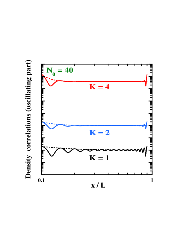
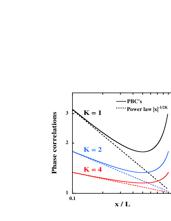
In Fig. 6 we have plotted the $m=1$ term of $\langle\rho(x)\rho(0)\rangle$ to illustrate how the density correlations are enhanced as $K$ is decreased. Thus for $K=1$ (free fermions or the Tonks limit of delta-interacting bosons) the distant points are more correlated in density than for large $K$ (very attractive fermions or bosons with weakly repulsive interactions). This means that the oscillatory terms become more important as $K$ decreases, whereas for large $K$ they can be safely neglected, as it is done in the Bogoliubov approximation. On the other hand, as shown in Fig. 7, distant points become less phase correlated for small $K$ as the result of density and phase being conjugated fields. The system is then said to be less “phase stiff”. However, for larger $K$ phase correlations are enhanced, and only in this sense one can speak of “Bose-Einstein condensate” even though, strictly speaking, there is not such a thing as a condensate (i.e. long range-order) in one dimension (for instance $\langle e^{i\phi(x)}\rangle_{\rm pbc}=0$). At most, all that exists in the thermodynamic limit is an algebraic decay of phase correlations, which is often called quasi long-range order (QLRO).

III.2 Open Boundary Conditions (OBC’s)

In this subsection we consider the ground state correlations for particles in a box. The expressions for the correlation functions in this case are somewhat more complicated than for periodic boundary conditions. The reason is that in a box translational invariance is lost and two-point correlation functions depend on both arguments separately and not only on their difference. Furthermore, the ground state expectation value of some operators becomes non-trivial, that is, there are non-trivial one-point correlation functions. This is the case of the density operator (see below). However, the operator $e^{i\phi(x)}$ continues to have zero-expectation value, implying the absence of any continuous symmetry-breaking even though the system is finite and bounded.

Figure 8: Phase correlations for a system of bosons in a box. In the left plot, $x^{\prime}$ has been fixed to the center of the box, while phase correlations are sample as $x$ is shifted towards the right end. In the right plot, $x^{\prime}$ is close to the left end and as $x$ increases we move towards the right end. As remarked in the case of a ring, the system becomes less phase stiff as $K$ is decreased. This means that in this case the boundary conditions have a large effect on the phase correlations in the Tonks limit ($K=1$) than in the weakly interacting limit ($K\gg 1$).

We first compute the ground state expectation value of the density:

$$\langle\rho(x)\rangle=\rho_{\rm o}\sum_{m=-\infty}^{+\infty}e^{2im\pi\rho_{0}x}\langle A_{2m,0}(x)\rangle_{\rm obc}=\rho_{0}\left\{1+\sum_{m>0}c_{m}\left[\frac{1}{\rho_{0}d(2x|2L)}\right]^{m^{2}K}\cos(2m\pi\rho_{0}x+\delta_{m})\right\},$$ (65)

where the coefficients $c_{m}$ and $\delta_{m}$ are model dependent coeffs . The above expression is valid in the scaling limit, which for the above expression means that $\min\{x,L-x\}\gg a$, i.e. sufficiently far from the boundaries. It is noticeable that $\langle\rho(x)\rangle$ exhibits Friedel oscillations, independently of the statistics of the constituent particles. This is not surprising in view of the many common features exhibited by interacting bosons and fermions in one-dimension, and whose origin was already discussed in Sect. II. In the thermodynamic limit, the replacement $d(2x|2L)\to|2x|$ shows that the different oscillating terms in the expression for $\langle\rho(x)\rangle$ decay from the boundary as power laws with increasingly large exponents: $m^{2}K$ for $m=1,2,\ldots$ indicating that only the leading two terms are important.

Next we consider the more complicated two-point correlation functions. We begin with the density-density correlation function,

$$\langle\rho(x)\rho(x^{\prime})\rangle = \left\{\frac{1}{\pi^{2}}\langle\partial_{x}\Theta(x)\partial_{x^{\prime}}\Theta(x^{\prime})\rangle_{\rm obc}+\sum_{m,m^{\prime}=-\infty}^{+\infty}e^{2i\pi\rho_{0}(mx-m^{\prime}x^{\prime})}\langle A_{2m,0}(x)A_{-2m^{\prime},0}(x^{\prime})\rangle_{\rm obc}\right\}$$ (66)

$$= \rho^{2}_{0}\>\Bigg{\{}1-\frac{K}{2\pi^{2}}\left[\frac{1}{\rho_{0}d(x-x^{\prime}|2L)}\right]^{2}-\frac{K}{2\pi^{2}}\left[\frac{1}{\rho_{0}d(x+x^{\prime}|2L)}\right]^{2}$$

$$+\sum_{m,m^{\prime}=-\infty}^{+\infty}a_{m,m^{\prime}}\left[\frac{d(x+x^{\prime}|2L)}{d(x-x^{\prime}|2L)}\right]^{2mm^{\prime}K}\frac{e^{2i\pi\rho_{0}(mx-m^{\prime}x^{\prime})}}{\left[\rho_{0}d(2x|2L)\right]^{m^{2}K}\left[\rho_{0}d(2x^{\prime}|2L)\right]^{m^{\prime 2}K}}\Bigg{\}}.$$

Using the results of Appendix D one can also obtain the one-particle density matrices of bosons and fermions. The corresponding expressions read:

$$\langle\Psi^{\dagger}(x)\Psi(x^{\prime})\rangle = \rho_{0}\sum_{m,m^{\prime}=-\infty}^{+\infty}e^{2i\pi\rho_{0}(mx-m^{\prime}x^{\prime})}\langle A_{2m,-1}(x)A_{-2m^{\prime},1}(x^{\prime})\rangle_{\rm obc}$$ (67)

$$= \rho_{0}\>\left[\frac{\rho^{-1}_{0}\sqrt{d(2x|2L)d(2x^{\prime}|2L)}}{d(x+x^{\prime}|2L)d(x-x^{\prime}|2L)}\right]^{\frac{1}{2K}}\sum_{m,m^{\prime}=-\infty}^{+\infty}b_{m,m^{\prime}}\>e^{-i(m+m^{\prime})\pi{\rm sgn}(x-x^{\prime})/2}$$

$$\times\left[\frac{d(x+x^{\prime}|2L)}{d(x-x^{\prime}|2L)}\right]^{2mm^{\prime}K}\frac{e^{2i\pi\rho_{0}(mx-m^{\prime}x^{\prime})}}{\left[\rho_{0}d(2x|2L)\right]^{m^{2}K}\left[\rho_{0}d(2x^{\prime}|2L)\right]^{m^{\prime 2}K}}$$

$$\langle\Psi^{\dagger}_{F}(x)\Psi_{F}(x^{\prime})\rangle = \rho_{0}\sum_{m,m^{\prime}=-\infty}^{+\infty}e^{2i\pi\rho_{0}\left[(m+\frac{1}{2})x-(m^{\prime}+\frac{1}{2})x^{\prime}\right]}\langle A_{2m+1,-1}(x)A_{-2m^{\prime}-1,1}(x^{\prime})\rangle_{\rm obc}$$ (68)

$$= \rho_{0}\>\left[\frac{\rho^{-1}_{0}\sqrt{d(2x|2L)d(2x^{\prime}|2L)}}{d(x+x^{\prime}|2L)d(x-x^{\prime}|2L)}\right]^{\frac{1}{2K}}\sum_{m,m^{\prime}=-\infty}^{+\infty}f_{m,m^{\prime}}\>e^{-i(m+m^{\prime}+1)\pi{\rm sgn}(x-x^{\prime})/2}$$

$$\times \left[\frac{d(x+x^{\prime}|2L)}{d(x-x^{\prime}|2L)}\right]^{2(m+\frac{1}{2})(m^{\prime}+\frac{1}{2})K}\frac{e^{2i\pi\rho_{0}\left[(m+\frac{1}{2})x-(m^{\prime}+\frac{1}{2})x^{\prime}\right]}}{\left[\rho_{0}d(2x|2L)\right]^{(m+\frac{1}{2})^{2}K}\left[\rho_{0}d(2x^{\prime}|2L)\right]^{(m^{\prime}+\frac{1}{2})^{2}K}}.$$

The coefficients $a_{m,m^{\prime}},b_{m,m^{\prime}}$ and $c_{m,m^{\prime}}$ are model-dependent complex numbers. In contrast with the case of periodic boundary conditions, where these prefactors can shown to be real, this cannot be established in the present case cft . The above expressions are accurate in the scaling limit, which for two-point correlation functions means that $|x-x^{\prime}|\gg a$ as well as $\min\{x,x^{\prime},L-x,L-x^{\prime}\}\gg a$. It is also worth mentioning that the bulk behavior is recovered for $|x-x^{\prime}|\ll\min\{x,x^{\prime},L-x,L-x^{\prime}\}$, i.e. mostly near the center of the box (see Fig. 8). In this limit, the less oscillating terms are those with $m=m^{\prime}$, which exhibit, in the thermodynamic limit, the same algebraic decay as the correlations for the ring geometry. It is also worth pointing out that in the Tonks limit (i.e. for $K=1$), the leading term of Eq. (67) agrees with the asymptotic result obtained in Ref. Forrester03, ,

$$\langle\Psi^{{\dagger}}(x)\Psi(x^{\prime})\rangle_{\rm obc}=\rho_{0}\,b^{\rm Tonks}_{00}\left[\frac{\rho^{-1}_{0}\sqrt{d(2x|2L)d(2x^{\prime}|2L)}}{d(x+x^{\prime}|2L)d(x-x^{\prime}|2L)}\right]^{\frac{1}{2}},$$ (69)

where $b^{\rm Tonks}_{00}=2^{-1/3}\sqrt{\pi e}\,A^{-6}\simeq 0.5214$ ($A\simeq 1.2824271$ is Glaisher’s constant). Note that this is the same prefactor as the one found for PBC’s, which is not suprising given that both correlation functions have the same bulk limit.

It is interesting to point out that for particles in a box there are two types of exponents that characterize the decay of correlation functions. Consider for instance the density correlation function, Eq. (66). Its bulk behavior (i.e. near the center of the box) is governed by the exponent $2m^{2}K$ for a harmonic that oscillates as $e^{\pm 2m\pi\rho_{0}(x-x^{\prime})}$. However, the asymptotic behavior when one of the coordinates is taken near the boundary is governed by a different exponent. Thus if we set $x^{\prime}\approx a$ and $x\gg x^{\prime}$, a term that oscillates as $e^{\pm 2im\pi\rho_{0}x}$in the correlation function falls off with the exponent equal to $m^{2}K$, i.e. the same exponent that we have already encountered for the Friedel oscillations of the density. For the boson density matrix the corresponding exponents are $m^{2}K+3/4K$ whereas for the fermions they are $(m+1/2)^{2}K+3/4K$. It is important to stress that the presence of the boundary breaks the (Lorentz) invariance of $H_{\rm eff}$ making space and time directions non-equivalent. To see this, consider a dynamic correlation function such like the Green’s function $\langle\Psi^{{\dagger}}(x,t)\Psi(x^{\prime},0)\rangle$, for bosons, or $\langle\Psi^{{\dagger}}_{F}(x,t)\Psi(x^{\prime},0)\rangle$, for fermions ($t>0$). Using the expressions of Appendix D, and performing the analytical continuation $\tau\to it$ after setting $x=x^{\prime}\approx a$, one obtains that the leading term decays as $t^{-1/K}$ for $t\gg a/v_{s}$ (for both bosons and fermions). This in contrast with the behavior of the same functions in the bulk, where space and time are equivalent (i.e. Lorentz invariance is restored) and one expects a behavior like $t^{-1/2K}$ for bosons and $t^{-(1/K+K)/2}$ for fermions.

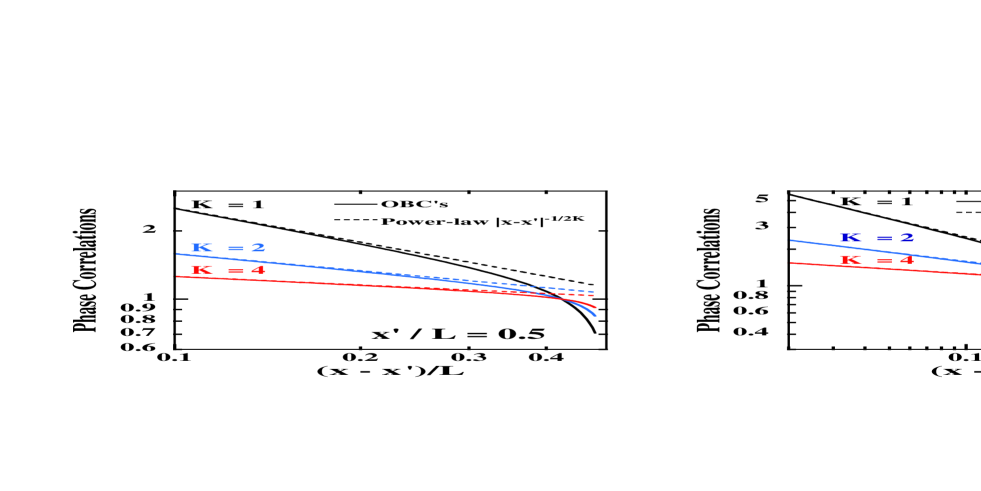
To illustrate both finite-size and confinement effects we show in Fig. 8 the behavior of leading term in Eq. (67), which corresponds to the phase fluctuations $\langle e^{-i\phi(x)}e^{i\phi(0)}\rangle_{\rm obc}$ (i..e. $m=m^{\prime}=0$). As mentioned above, the correlation function is now a function of $x$ and $x^{\prime}$ separately. Thus, in Fig. 8 we have considered two situations. In the plot on the left, we take $x^{\prime}$ to be the center of the box. Thus it can be seen that the power-law (bulk) behavior is a good approximation for $x$ around $L/2$, whereas the phase correlations deviate from it as $x$ approaches the right end of the box (i.e. for $x-x^{\prime}\gtrsim 0.3L$. These deviations become more important as $K$ is decreased and the system approaches the Tonks limit ($K=1$). This is because, as remarked in the previous subsection, the system becomes less phase stiff as $K$ decreases. Thus, for smaller $K$ the boundary conditions have a larger effect in decreasing the phase correlations near the ends of the box. However, for larger $K$ the system exhibits a larger phase stiffness, and phase correlations decay very slowly, even near the boundaries. Furthermore, the deviations from the power-law behavior are smaller. However, these deviations become much larger with distance if now $x^{\prime}=0.1L$, i.e. when $x^{\prime}$ is fixed near the left end of the box. Then, the bulk power-law is no longer a good approximation and we can observe deviations from it for a decade: from $x-x^{\prime}\approx 0.1L$ to $x-x^{\prime}\approx L$. The reasons for this deviations is that initially the correlations decay according to the bulk power-law, but they rapidly cross-over to a decay governed by the exponent $3/4K$ (recall that $m=m^{\prime}=0$). Near the right boundary, the correlation function must vanish. This is because the pinning of the density field $\Theta(x)$ at $x=L$ makes fluctuate the phase at that point wildly.

III.3 Correlations at finite temperature

As described in Appendix C the same methods that have allowed us to obtain the correlation functions of a finite ring at zero temperature also allow to obtain expressions for the correlation functions of an infinite system at finite temperature (see below).

At finite temperature one finds (see Appendix C) that correlations decay exponentially with distance (as opposed to the algebraic decay found at $T=0$ for $L\to+\infty$). Therefore, in the expressions below, we shall keep only the leading terms, which effectively means that we cut-off the series of harmonics at $m=0$ (for the boson density matrix, and at $|m|=1$ for the density correlation function and the fermion density matrix. Thus the following expressions are obtained:

$$\langle\rho(x)\rho(0)\rangle_{T} = \rho^{2}_{0}\left\{1-\frac{K}{2\pi^{2}}\left[\frac{\pi/L_{T}}{\rho_{0}\sinh\left(\pi x/L_{T}\right)}\right]^{2}+B\cos(2\pi\rho_{0}x)\left[\frac{\pi/L_{T}}{\rho_{0}\sinh\left(\pi x/L_{T}\right)}\right]^{2K}+\ldots\right\},$$ (70)

$$\langle\Psi^{{\dagger}}(x)\Psi(0)\rangle = \rho_{0}\>A\left[\frac{\pi/L_{T}}{\rho_{0}\sinh\left(\pi x/L_{T}\right)}\right]^{\frac{1}{2K}}+\ldots,$$ (71)

$$\langle\Psi^{{\dagger}}_{F}(x)\Psi_{F}(0)\rangle_{T} = \rho_{0}\>C\left[\frac{\pi/L_{T}}{\rho_{0}\sinh\left(\pi x/L_{T}\right)}\right]^{\frac{K}{2}+\frac{1}{2K}}\sin|\pi\rho_{0}x|+\ldots,$$ (72)

the dimensionless coefficients $A,B$, and $C$ are model dependent. In Sect. IV.2 we shall discuss how to fix the prefactor for the bosonic density matrix, Eq. (71).

From the previous expressions one can see that the behavior of the correlations “crosses over” from algebraic decay for $a\ll|x|\lesssim L_{T}$ to exponential $\sim\exp\left[-|x|/L_{c}(T)\right]$ for $|x|\gg L_{c}(T)$. The characteristic decay length $L_{c}(T)$ depends on the correlation function. Thus, for the non-oscillating part of $\langle\rho(x)\rho(0)\rangle_{T}$, $L_{c}(T)\sim L_{T}$. However, for the oscillating part $L_{c}(T)\sim L_{\rho}(T)=\hbar v_{s}/\pi KT=\hbar v_{N}/\pi T$. For the phase correlations, however, the characteristic distance is of the order of $L_{\phi}(T)=\hbar v_{s}K/\pi T=\hbar v_{J}/\pi T=\hbar^{2}\rho_{0}/MT$, the latter expression being valid only in systems with Galilean invariance. One can use the previous expressions also in finite-size systems provided the temperature is high enough. The value of $T$ for which these characteristic lengths become of the order of the system size, $L$, give us a rough estimate of the temperature scale below which finite-size and confinement effects are important. Since, in general, $L_{T}\neq L_{\phi}\neq L_{\rho}$, this temperature scale depends on the correlation function. Thus, for the phase correlations, $L_{\phi}(T)\approx L$ for $T_{\phi}\approx\hbar v_{J}/\pi L=\hbar^{2}\rho_{0}/ML$, the latter expression applying to systems with Galilean invariance. However, for the density correlations, $L_{T}/\pi\approx L$ or $L_{\rho}(T)\approx L$, whichever gives the highest value of $T$. Hence, $T_{\rho}=\max\{\hbar v_{s}/\pi L,\hbar v_{s}/\pi KL\}$.

IV Delta-Interacting bosons as a Luttinger liquid

IV.1 Extracting the Luttinger liquid parameters from the Bethe-ansatz solution

Figure 9: Density and phase stiffness as a function of $\gamma=Mg/\hbar^{2}\rho_{0}$. The dots are the result of the numerical calculation of $v_{J}$ from the Bethe-ansatz equations. The dashed line corresponds to the Bogoliubov result for $v_{N}$, Eq. (76). The dotted-dashed line is the large-$\gamma$ asymptotic result, Eq. (77).

In what follows, we shall illustrate many of the concepts introduced above by considering a model of bosons interacting with a zero-range potential Lieb63a ; Lieb63b . This is relevant to cold atomic vapors, where atoms mainly interact through the s-wave scattering channel, and their interaction is parametrized by the s-wave scattering length, $a_{s}$. Olshanii Olshanii98 has shown that the interaction between atoms confined in 1D wave guide with transverse harmonic confinement is well described by a zero-range interaction potential $v(x-x^{\prime})=g\>\delta(x-x^{\prime})$, where

$$g=\frac{4\hbar^{2}}{M\ell_{\perp}}\frac{a_{s}/\ell_{\perp}}{1-C(a_{s}/\ell_{\perp})},$$ (73)

where $a_{s}$ is the three-dimensional scattering length, $C=1.4603\ldots$, and $\ell_{\perp}=\sqrt{\hbar/M\omega_{\perp}}$ is the transverse oscillator length. There is a single dimensionless parameter, $\gamma=Mg/\hbar^{2}\rho_{0}$, which characterizes the different regimes (some authors prefer to use the 1D gas parameter $\rho_{0}|a_{1D}|$, which is related to $\gamma$ by $\gamma=2/\rho_{0}|a_{1D}|$).

Figure 10: Luttinger-liquid parameters vs. $\gamma=Mg/\hbar^{2}\rho_{0}$. The dashed lines are the small $\gamma$ approximations obtained from Bogoliubov theory whereas the dotted-dashed lines correspond to the asymptotic expressions for large $\gamma$.

The model thus defined is exactly solvable. Its solution for periodic boundary conditions was found by Lieb and Liniger Lieb63a ; Lieb63b , whereas the case with open boundary conditions was solved by Gaudin Gaudin71 . Lieb and Liniger were also able to compute the ground state energy per particle as well as the chemical potential and the sound velocity by numerically solving a set of integral equations. One can thus obtain the phase and density stiffness, $v_{J}$ and $v_{N}$, by writing integral equations which allow one to obtain these parameters. These equations were written down by Haldane Haldane81c . However, we shall not follow this path here but instead, we shall adopt a different approach Schulz90 ; Mironov91 . We first numerically find the solution of the Bethe-ansatz equations Lieb63a ; Gaudin80 ,

$$k_{i}L=2\pi I_{i}+\alpha-2\sum_{j=1}^{N_{0}}\tan^{-1}\left(\frac{k_{i}-k_{j}}{\gamma\rho_{0}}\right).$$ (74)

When deriving these equations we have assumed that the boundary conditions are not periodic but twisted as in (32), where $\alpha$ is the twist in the phase. In the ground state the set of integers $\left\{I_{i}\right\}_{i=1,\ldots,N_{0}}=\left\{-(N_{0}-1)/2,-(N_{0}-3)/2,\ldots,(N_{0}-3)/2,(N_{0}-1)/2\right\}$ Lieb63a ; Gaudin80 . The ground state energy for $N_{0}$ particles and a phase twist $\alpha$ can be computed from the solution to the above equations,

$$E_{0}(N_{0},\alpha)=\sum_{i=1}^{N_{0}}\frac{\hbar^{2}k^{2}_{i}}{2M}$$ (75)

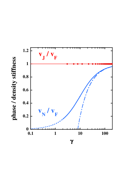
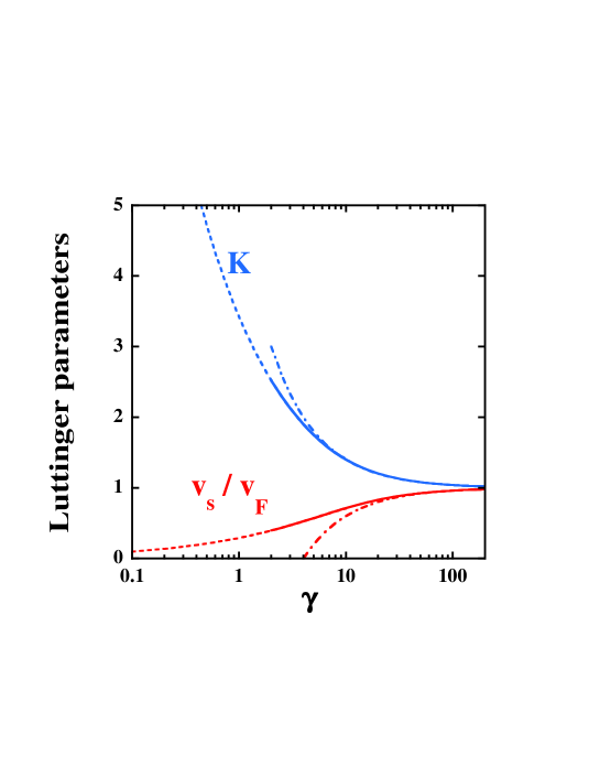
and using Eq. (31) and (37) $v_{N}$ and $v_{J}$ can be numerically computed . The results of these calculations are shown in figures 9 and 10. Fig. 9 shows the behavior of the phase ($v_{J}$) and density stiffness ($v_{N}$) as a function of the dimensionless parameter $\gamma=Mg/\hbar^{2}\rho_{0}$. We have numerically obtained $v_{J}$ to show explicitly that, because of the Galilean invariance of the model, $v_{J}=v_{F}$.

As already pointed out by Lieb and Liniger Lieb63a ; Lieb63b , the Bogoliubov approximation for the ground state energy yields a very accurate expression of the sound velocity for $\gamma\lesssim 10$. Hence,

$$v_{N}=v_{F}\left(\frac{\gamma}{\pi^{2}}\right)\left(1-\frac{\sqrt{\gamma}}{2\pi}\right).$$ (76)

However, for $\gamma\gg 1$ one can extract an asymptotic expression for $v_{N}$ from either the expressions for $\mu$ obtained for large $\gamma$ by Lieb and Liniger Lieb63a or from a strong coupling expansion of energy Haldane81a ; Cazalilla03 , which yields:

$$v_{N}=v_{F}\left(1-\frac{8}{\gamma}\right)$$ (77)

In Fig. 10 we have plotted the parameters $v_{s}$ and $K$ as function of $\gamma$. They also show good agreement with the asymptotic results at small $\gamma$,

$$v_{s} = v_{F}\>\frac{\sqrt{\gamma}}{\pi}\left(1-\frac{\sqrt{\gamma}}{2\pi}\right)^{1/2},$$ (78)

$$K = \frac{\pi}{\sqrt{\gamma}}\left(1-\frac{\sqrt{\gamma}}{2\pi}\right)^{-1/2},$$ (79)

and large $\gamma$,

$$v_{s} = v_{F}\left(1-\frac{4}{\gamma}\right),$$ (80)

$$K = \left(1+\frac{4}{\gamma}\right).$$ (81)

From Fig. 10 one can see that as $\gamma$ varies from zero to infinity, $K$ varies from infinity to $1$. Thus, $K=1$ corresponds to the Tonks limit, which is also the value of $K$ for non-interacting fermions. Finally, in table 1 we provide a “translation table” between $K$ and $\gamma$ for the values of $K$ used in plots of this article.

Table 1: Translation table $\gamma$ to $K$ for some values of $K$ used in this paper.

$\gamma$	$K$
$+\infty$	$1$
$3.517$	$2$
$0.7126$	$4$

IV.2 Remarks on cut-offs and prefactors

One of the disadvantages of the harmonic-fluid approach is that it cannot provide explicit expressions for the prefactors of the correlation functions. As obtained within this approach, they are cut-off dependent quantities and their values depend on the particular regularization scheme used in the calculation This is a signature of non-universality, i.e. the prefactors depend on the microscopic details of the model. Thus, they must be fixed by other means, either by comparing with numerical results or by adopting a physically sensible regularization scheme (this is possible in certain models) and using rather sophisticated form-factor methods (see e.g. GNT98 and references therein). Sometimes expressions for the prefactors can be obtained in certain limits by working directly with the microscopic model. This is the case for the Tonks limit of delta-interacting bosons Lenard72 ; VaidyaTracy79 or for a number of lattice models, such like the quantum-Ising model and or the XY model Lieb61 ; McCoy68 .

Figure 11: Large momentum cut-off vs. $\gamma$. At large $\gamma$, $q_{c}\to\pi\rho_{0}/2$, whereas for small $\gamma$, $q_{c}\approx\xi^{-1}=\sqrt{\mu\rho_{0}}/\hbar$, i.e. the inverse healing length.

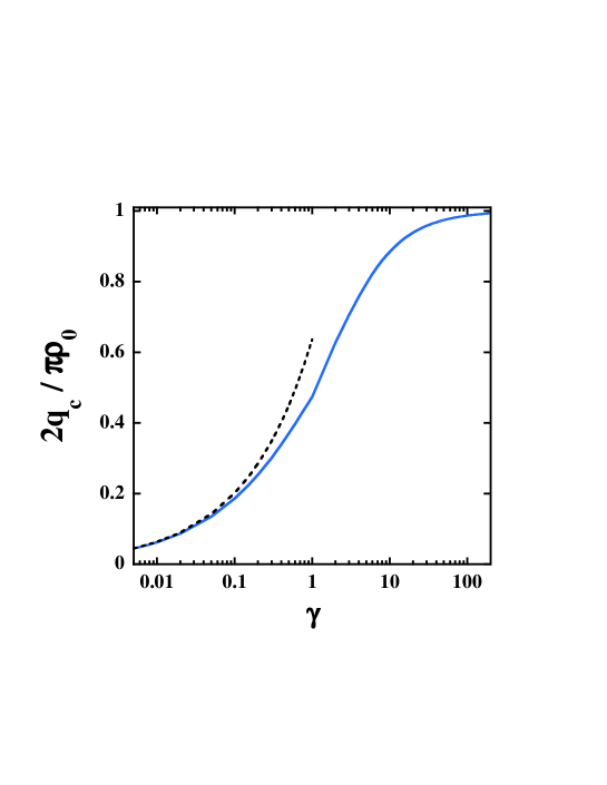
Before jumping into the discussion of the prefactors for the model of delta-interacting bosons, let us pause for a moment to consider a question that will be relevant for the fixing of the prefactors, namely the dependence of the wave-number cut-off $q_{c}=\mu/\hbar v_{s}$ on $\gamma$. As mentioned in previous sections, for delta-interacting bosons the different regimes are characterized by a single dimensionless parameter, $\gamma=Mg/\hbar^{2}\rho_{0}$, where $g$ is the strength of the interaction. For weakly interacting bosons (i.e. $\gamma\to 0$) $q_{c}\to\xi^{-1}=\gamma^{1/2}\rho_{0}$, where $\xi=\hbar/\sqrt{M\mu}$ is the healing length. On the other hand, for strongly interacting bosons ($\gamma\to+\infty$), $q_{c}\to\pi\rho_{0}/2$. The full dependence can be obtained from the numerical solution of the Bethe-ansatz equations (74). The result for $q_{c}$ has been plotted in Fig. 11.

As we have mentioned at the beginning of this section, within the harmonic-fluid approach the prefactors depend of the cut-off, $a\lesssim q^{-1}_{c}$ (see Appendix C). In the weakly interacting regime, Popov Popov80 ; Mora02 was able to obtain the prefactor of the one-body density matrix . In our notation, his result reads:

$$g_{1}(x)=\langle\Psi^{{\dagger}}(x)\Psi(0)\rangle=\rho_{0}\left(\frac{e^{2-C}\xi}{4|x|}\right)^{\sqrt{\gamma}/2\pi},$$ (82)

for $\gamma\ll 1$. In the previous expression $C=0.57721\ldots$ is Euler’s constant and $\xi$ the healing length, $\xi=\rho^{-1}_{0}\gamma^{-1/2}$. Taking into account that the numerical factor $e^{2-C}/4=1.037\simeq 1$, we notice that the above result can be obtained within the harmonic-fluid approach by setting the short-distance cut-off $a=\xi$. Indeed, this makes a lot of sense since, as discussed above, in the weakly interacting limit one expects that $a=q^{-1}_{c}=\xi$. Things become more interesting when one expresses both the exponent and the prefactor in terms of the Luttinger-liquid parameter $K$, so that one can make contact with the way $g_{1}(x)$ was written in previous sections,

$$\langle\Psi^{{\dagger}}(x)\Psi(0)\rangle=\rho_{0}\frac{A_{\rm Popov}(K)}{|\rho_{0}x|^{1/2K}},$$ (83)

where we have used that, in the weakly interacting limit, $K=\pi\gamma^{-1/2}\gg 1$. The dimensionless prefactor (neglecting the difference $e^{2-C}/4-1\simeq 0.037$) is

$$A_{\rm Popov}(K)=\left(\frac{K}{\pi}\right)^{1/2K}.$$ (84)

In view of this result, one may be very tempted to use this expression for any value of $K$ relevant to this model (i.e. $1\leq K<+\infty$). The result, when compared with the diffusion Monte Carlo data reported in Ref. Giorgini02, and exact results Lenard72 ; VaidyaTracy79 ; Forrester03 , is very surprising (see Table 2). It is found that Eq. (84) is accurate within less than $10\%$ over the whole range of $K$ values, becoming essentially exact for $K\gg 1$, as expected. This fact is quite remarkable taking into account that from $K\approx 10$ to $K=1$ the prefactor changes by a almost a factor of two.

Table 2: Numerical prefactor of the one-body density matrix as obtained from Eq. (84) vs. exact and diffusion Monte Carlo (DMC) results.

$\gamma=Mg/\hbar^{2}\rho_{0}$	$K$	$K$ from the exponent (Exact/DMC)	$A_{\rm Popov}(K)$	$A_{\rm Exact/DMC}$
$+\infty$	$1$	1	$0.5642$	$0.5214$
$2\times 10^{3}$	$1.002$	$1.0$	$0.565$	$0.530$
$6.6667$	$1.584$	$1.582$	$0.806$	$0.760$
$2.0$	$2.523$	$2.525$	$0.957$	$0.951$
$0.0667$	$12.425$	$12.469$	$1.06$	$1.06$
$2\times 10^{-3}$	$70.50$	$70.42$	$1.02$	$1.02$

IV.3 Tips to compare with the experiments in cold gases

In the previous sections we have equipped ourselves with the tools to characterize the behavior of one-dimensional cold-atom systems. In this characterization the Luttinger-liquid parameters $v_{s}$ and $K$ play an prominent role. The latter is especially important because it enters the exponents of the correlation functions, and governs their algebraic decay at zero temperature. Furthermore, the value of $K$ also tells us to which kind of instabilities the system can become unstable when perturbed. A well-known example Haldane81b ; Buchler03 is the quantum-phase transition to a Mott-insulator in the presence of a commensurate periodic potential, which takes place (strictly speaking at $T=0$ and $L\to\infty$) for arbitrarily weak potentials at $K<2$. At finite temperature, the behavior of the system is characterized by the correlation lengths $L_{T}$, $L_{\phi}(T)$ and $L_{\rho}(T)$, which are combinations of the parameters $v_{s},K$ and the temperature, $T$. As we are interested in the bulk properties of 1D systems, we shall focus in this section on the implications of the correlation functions previously derived for the experimental observations.

Figure 12: Momentum distribution at finite temperature for the Tonks gas ($K=1$). The inset shows that the asymptotic behavior is not as $p^{-2}$, as expected for a lorentzian but rather as $p^{1/2K-1}=p^{-1/2}$.

We begin our discussion by considering the finite temperature momentum distribution. This quantity can be accessed by performing Bragg scattering measurements at large momentum transfer Richard03 ; Grebier03 ; Luxat03 . At temperatures $T\gg T_{\phi}=\hbar^{2}\rho_{0}/ML$, one can safely neglect finite-size and boundary effects. In this temperature range the effects of the inhomogeneity in harmonically trapped systems can be treated using the local density approximation as described in Refs. Richard03, ; Grebier03, . For a uniform system, the momentum distribution is defined as the Fourier transform of $g_{1}(x,T)$, i.e.

$$n(p,T)\simeq\int_{-\infty}^{+\infty}dx\,e^{-ipx}\>g_{1}(x,T)$$ (85)

After introducing Eq. (71) into this expression and approximating the prefactor by $A_{\rm Popov}(K)=(K/\pi)^{1/2K}$, we obtain the following expression:

$$n(p,T)\simeq\left(\frac{2K}{\pi}\right)^{1/2K}\left(\frac{\rho_{0}L_{\phi}(T)}{K}\right)^{1-\frac{1}{2K}}\Gamma\left(1-\frac{1}{2K}\right){\rm Re}\left[\frac{\Gamma\left(1/4K+ipL_{\phi}(T)/2K\right)}{\Gamma\left(1-1/4K+ipL_{\phi}(T)/2K\right)}\right]$$ (86)

where $L_{\phi}(T)=\hbar^{2}\rho_{0}/MT=\rho_{0}\Lambda^{2}_{T}$ ($\Lambda_{T}=\hbar/\sqrt{MT}$ is the de Broglie thermal wave-length) is the phase correlation length. This expression for $n(p,T)$ is different from the lorentzian form commonly used throughout the literature. The lorentzian results from taking the Fourier transform of

$$g_{1}(x,T)\simeq\rho_{0}\left(\frac{K^{2}}{\pi\rho_{0}L_{\phi}(T)}\right)^{1/2K}e^{-|x|/2L_{\phi}(T)},$$ (87)

which is the asymptotic form of $g_{1}(x,T)$ for $|x|\gg L_{T}$. Hence,

Figure 13: Momentum distribution at finite temperature for a system with $K=2$. The inset shows that the asymptotic behavior is not as $p^{-2}$, but rather as $p^{1/2K-1}=p^{-3/4}$.

$$n^{\prime}(p,T)\simeq 4\left(\frac{K^{2}}{\pi}\right)^{\frac{1}{2K}}\left(\rho_{0}L_{\phi}(T)\right)^{1-1/2K}\frac{1}{1+\left(2pL_{\phi}(T)\right)^{2}}.$$ (88)

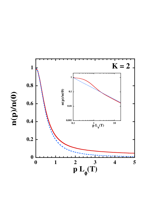
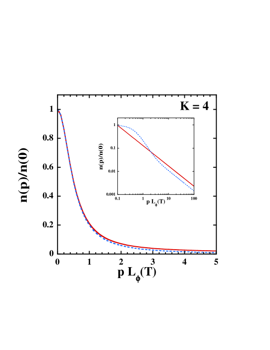
In Figs. 12, 13, and 14 we compare both forms, Eq.(86) and (88); $n(p,T)/n(0,T)$ and $n^{\prime}(p,T)/n^{\prime}(0,T)$ are plotted against $pL_{\phi}(T)$. Our calculations assume the scaling limit, which in these plots means that $|p|\lesssim q_{c}$. For $|p|\gg q_{c}$, Olshanii and Dunjko have shown Olshanii02 that $n(p,T)\sim p^{-4}$. From figures 12, 13, and 14 one can draw the conclusion that the lorentzian is a good approximation for large $K$, i.e. for weakly interacting bosons. The width of the lorentzian is proportional to $L_{\phi}(T)\propto\rho_{0}/T$, which thus provides a measure of this ratio. However, in the Tonks limit the momentum distribution at $T>T_{\phi}$ looks more like a stretched lorentzian. The reason is that, in the large momentum limit, $n(p,T)$ as given by Eq. (87), behaves as a power-law: $p^{-(1-1/2K)}\sim p^{-1/2}$, for $K=1$. Experimentally, extracting the Luttinger-liquid parameter from $n(p,T)$ may be hard because the true $n(p,T)$ may not display this algebraic behavior in a sufficiently wide range of $p$ (set aside the complications that averaging $g_{1}$ using the local density approximation may introduce). However, there may be some chance to observe the more qualitative behavior shown by these plots: as the system’s parameters are tuned (e.g. by using a Feshbach or the confinement-induced resonance Olshanii98 ) towards the Tonks limit, the momentum distribution should become more “stretched” and less Lorentzian-like.

Figure 14: Momentum distribution at finite temperature for a system with $K=4$. The inset shows that the asymptotic behavior is not as $p^{-2}$, but rather as $p^{1/2K-1}=p^{-7/8}$.

A more quantitative estimate of the Luttinger-liquid parameters near the center of the trap can be obtained from the dynamic density response function,

$$\chi(q,\omega) = \int dx\>dt\,e^{i\omega t-iqx}\>\chi(x,t),$$ (89)

$$\chi(x,t) = -\frac{i}{\hbar}\theta(t)\>\langle\left[\rho(x,t),\rho(0,0)\right]\rangle_{T},$$ (90)

whose imaginary part is measured in low-momentum Bragg scattering experiments Zambelli00 . In the low momentum ($=$ long wave-length) limit, we can replace $\rho(x,t)$ by $\Pi(x,t)=\partial_{x}\theta(x,t)/\pi$. Thus, using the equations of motion for $\Pi(x,t)$, one can obtain the result ($\eta\to 0^{+}$):

$$\chi(q,\omega)=-\frac{q^{2}}{\pi\hbar}\frac{v_{J}}{(\omega+i\eta)^{2}-\omega^{2}(q)},$$ (91)

where $\omega(q)=v_{s}|q|$ for $|q|\ll q_{c}$. Hence,

$${\rm Im}\>\chi(q,\omega)=\frac{v_{J}q^{2}}{2\hbar\omega(q)}\left[\delta\left(\omega-\omega(q)\right)-\delta\left(\omega+\omega(q)\right)\right].$$ (92)

Since $v_{J}=v_{s}K$, the weight becomes $Kq/2$. Thus by measuring the dispersion $\omega(q)$ one can obtain $v_{s}$, whereas from the weight of ${\rm Im}\chi(q,\omega)$, $K$ can be measured. Inhomogeneity effects can be treated also in this case within the local density approximation, as discussed in Ref. Zambelli00, . In this respect, we notice that ${\rm Im}\>\chi(q,\omega)$ has the same structure as the result from Bogoliubov approximation in $d>1$. The only difference is that it holds, as well as the expression for $n(p,T)$ derived above, for all values of the interaction parameter $\gamma$, and not only in the weakly interacting limit.

V Jastrow-Bijl wave functions and Luttinger liquids

In Sect. II it has been shown that the low-energy spectrum of a Luttinger liquid is completely exhausted by phonons with linear dispersion. This phonons are nothing but collective oscillations of the density and the phase. In view of this fact, one may wonder what kind of correlations are built into the ground state wave function by these collective excitations. The question has been considered in different contexts by several authors ReattoChester67 ; Pham9901 . Here we restrict ourselves to the case of particles in a box (OBC’s). Taking inspiration from the work of Reatto and Chester ReattoChester67 we write the ground state wave function for $N_{0}$ bosons in a box as follows:

$$\Phi_{0}(x_{1},\ldots,x_{N})=\Phi_{c}(x_{1},\ldots,x_{N})\tilde{\Phi}_{0}(x_{1},\ldots,x_{N}).$$ (93)

where $\Phi_{c}(x_{1},\ldots,x_{N})$ describes the correlations between the particles in the ground state whereas $\tilde{\Phi}_{0}(x_{1},\ldots,x_{N})$ describes their independent motion, which for $N_{0}$ bosons in a box is given by

$$\tilde{\Phi}_{0}(x_{1},\ldots,x_{N_{0}})=\prod_{i=1}^{N_{0}}\sin\left(\frac{\pi x_{i}}{L}\right),$$ (94)

that is, all the $N_{0}$ lie in the lowest-energy orbital $\sin(\pi x/L)$. As for $\Phi_{c}(x_{1},\ldots,x_{N_{0}})$ we will obtain an asymptotic expression valid for $|x_{i}-x_{j}|\gg a$, for $i,j=1,\ldots,N_{0}$. In this limit the correlations between particles are dominated by the zero-point motion of the collective excitations.

In order to obtain the asymptotic behavior of $\Phi_{c}$, we consider the ground-state wave function of the low-energy Hamiltonian (in this section $\hat{A}$ denotes the operator of the corresponding classical variable $A$),

$$\hat{H}_{\rm eff}=\frac{\hbar v_{s}}{2}\int_{0}^{L}dx\>\left[\frac{\pi}{K}\hat{\Pi}^{2}(x)+\frac{K}{\pi}\left(\partial_{x}\hat{\phi}(x)\right)^{2}\right].$$ (95)

For OBC’s, it is convenient to use the following expansions:

$$\hat{\Pi}(x) = \hat{\Pi}_{0}+\sqrt{\frac{2}{L}}\sum_{q>0}\hat{\Pi}_{q}\,\cos(qx),$$ (96)

$$\hat{\phi}(x) = \hat{\phi}_{0}+\sqrt{\frac{2}{L}}\sum_{q>0}\hat{\phi}_{q}\,\cos(qx),$$ (97)

where $q=n\pi/L$, with $n$ a positive integer and $\hat{\Pi}_{0}=\hat{N}-N_{0}$ . The canonical commutation relations now read

$$\left[\hat{\Pi}_{0},\hat{\phi}_{0}\right] = i,$$ (98)

$$\left[\hat{\Pi}_{q},\hat{\phi}_{q^{\prime}}\right] = i\,\delta_{q,q^{\prime}}.$$ (99)

We shall work in first quantization, which means that the wave function $\Phi_{c}$ is regarded as functional of $\Pi(x)$. From the second of the above commutation rules

$$\hat{\phi}_{q}=-i\frac{\partial}{\partial\Pi_{q}}.$$ (100)

Therefore, when expressed in terms of Fourier modes the Hamiltonian takes the form

$$\hat{H}_{\rm eff}=\frac{\hbar\pi v_{s}}{2K}\sum_{q>0}\left[\hat{\Pi}^{2}_{q}+\left(\frac{qK}{\pi}\right)^{2}\hat{\phi}^{2}_{q}\right]=\frac{\hbar\pi v_{s}}{2K}\sum_{q>0}\left[\Pi^{2}_{q}-\left(\frac{qK}{\pi}\right)^{2}\frac{\partial}{\partial\Pi^{2}_{q}}\right],$$ (101)

i.e. it represents a collection of decoupled harmonic oscillators, and therefore its ground state is just a product of gaussians:

$$\Phi_{c}=\exp\left\{-\frac{\pi}{2K}\sum_{q>0}{\frac{\Pi^{2}_{q}}{q}}\right\}.$$ (102)

When expressed in terms of $\Pi(x)$, this function becomes:

$$\Phi_{c}=\exp\left\{\frac{1}{2}\int_{0}^{L}dx\int_{0}^{L}dx^{\prime}\>\Pi(x){\cal K}(x,x^{\prime})\Pi(x^{\prime})\right\},$$ (103)

where

$${\cal K}(x,x^{\prime})=-\frac{2\pi}{LK}\sum_{q>0}\frac{e^{-aq}}{q}\cos(qx)\cos(qx^{\prime})\simeq\frac{1}{K}\ln\left|4\sin\left[\frac{\pi(x+x^{\prime})}{2L}\right]\sin\left[\frac{\pi(x-x^{\prime})}{2L}\right]\right|.$$ (104)

Notice that $K(x,x^{\prime})$ depends on the short-distance cut-off $a$ and therefore, it cannot correctly describe short-distance correlations where $x\approx x^{\prime}$. The second expression above is thus only asymptotically correct.

As we discussed in Sect. II, the configurations of $\Pi(x)$ describe long wave-length density fluctuations, i.e. the “slow” part of the density. Thus, we are quite tempted to make the replacement $\Pi(x)\to\rho(x)=\sum_{i=1}^{N_{0}}\delta(x_{i}-x_{j})$. However, in doing this we must be careful enough to remove the terms that involve the function $K(x,x^{\prime})$ evaluated at $x=x^{\prime}$ since $K(x,x^{\prime})$ cannot describe short-distance correlations (In Ref. Cazalilla02 we failed to notice this, and as a result the wave function obtained there is not completely correct. See below for the correct expression). If we do so, the following function is obtained in terms of particle coordinates:

$$\Phi_{c}(x_{1},\ldots,x_{N_{0}})=\prod_{i<j}\left|\sin\left[\frac{\pi(x_{i}+x_{j})}{2L}\right]\sin\left[\frac{\pi(x_{i}-x_{j})}{2L}\right]\right|^{\frac{1}{K}}=\frac{1}{2^{N_{0}(N_{0}-1)}}\prod_{i<j}\left|\cos\left(\frac{\pi x_{i}}{L}\right)-\cos\left(\frac{\pi x_{j}}{L}\right)\right|^{1/K},$$ (105)

Hence, the complete ground-state wave function reads

$$\Phi_{0}(x_{1},\ldots,x_{N_{0}})={\cal N}\prod_{i<j}\left|\cos\left(\frac{\pi x_{i}}{L}\right)-\cos\left(\frac{\pi x_{j}}{L}\right)\right|^{1/K}\prod_{i=1}^{N_{0}}\sin\left(\frac{\pi x_{i}}{L}\right)$$ (106)

where $\cal N$ is the normalization constant.

There are several reasons to believe that the wave function (106) is, at least asymptotically, correct. First, in the non-interacting limit $K\to+\infty$ (i.e. $\gamma\to 0$ for delta-interacting bosons), $\Phi_{c}\to 1$, and one recovers the independent-particle ground state $\Phi_{0}=\tilde{\Phi}_{0}$. On the other hand, in the Tonks limit $K=1$, $\Phi_{0}$ is the exact ground state of a system of hard-core bosons in a box Forrester03 . Furthermore, if one repeats the above calculation for bosons in a ring, the result is the well-know Jastrow-Bijl function:

$$\Phi^{\rm ring}_{0}(x,\ldots,x_{N_{0}})={\cal N}\,\prod_{i<j}\left|\sin\left[\frac{\pi(x_{i}-x_{j})}{L}\right]\right|^{\frac{1}{K}}$$ (107)

It turns out that this is the exact ground state wave function of the Calogero-Sutherland model Sutherland98 , which is a model of hard-core bosons with long-range interactions, and whose Hamiltonian reads:

$$H_{CS}=-\frac{\hbar^{2}}{2M}\sum_{i=1}^{N_{0}}\frac{\partial^{2}}{\partial x^{2}_{i}}+\frac{\hbar^{2}}{M}\sum_{i<j}\frac{K^{-1}(K^{-1}-1)}{\left[d(x_{i}-x_{j}|L)\right]^{2}}.$$ (108)

It is also known that this model also has a solution under harmonic confinement Sutherland98 , i.e. for

$$H^{\prime}_{\rm CS}=-\frac{\hbar^{2}}{2M}\sum_{i=1}^{N_{0}}\frac{\partial^{2}}{\partial x^{2}_{i}}+\frac{M\omega^{2}}{2}\sum_{i=1}^{N_{0}}x^{2}_{i}+\frac{\hbar^{2}}{M}\sum_{i<j}\frac{K^{-1}(K^{-1}-1)}{(x_{i}-x_{j})^{2}}.$$ (109)

The exact ground-state wave function has a similar structure to Eq. (106):

$$\Phi_{0}(x,\ldots,x_{N_{0}})=\prod_{i<j}|x_{i}-x_{j}|^{1/K}\,\prod_{i=1}^{N_{0}}e^{-M\omega x^{2}_{i}/2\hbar}.$$ (110)

There is also a good chance that the latter wave function may be asymptotically correct for other models of interacting bosons in a harmonic trap.

VI Conclusions

In this paper we have addressed the properties of one-dimensional systems of cold atoms using the harmonic-fluid approach (also know as “bosonization”). Besides reviewing the method in pedagogical detail, we have argued that it allows to treat boson and fermion systems both in strongly and weakly interacting limits. We have also shown how concepts and results obtained using the Bogoliubov-Popov approach Popov ; Popov80 and its modifications Andersen02 ; Mora02 can be naturally recovered using bosonization, which in our opinion is much simpler conceptually. When combined with the conformal field theory methods explained in the appendices, it becomes a very powerful tool to obtain the functional forms of the correlation functions for various geometries (ring, box with Dirichlet BC’s), and also finite-temperature correlations. The method has some limitations, however, as it cannot provide explicit expressions for the prefactors of the correlation functions, which turn out to be model-dependent. Moreover, for strongly interacting systems it becomes difficult, without further input, to relate the phenomenological parameters $v_{J}$ and $v_{N}$ to the microscopic parameters of the model at hand. Nevertheless, for a relevant model of bosonic cold atoms, we have shown that one can successfully extract those parameters from the exact (Bethe-ansatz) solution. Furthermore, the prefactor of the one-body density matrix could be fixed with less than $10\%$ error by expressing a result obtained in the weakly interacting limit Popov80 in terms of $K=\sqrt{v_{J}/v_{N}}$. These results should allow for a quantitative comparison with the experiment. In this respect, we have discussed how to extract the Luttinger-liquid parameters $K$ and $v_{s}=\sqrt{v_{N}v_{J}}$ (i.e. the sound velocity) from Bragg-scattering measurements of the density response function and finite-temperature momentum distribution. For the latter quantity, we have argued that, as a system is tuned into the Tonks regime, the finite-$T$ momentum distribution should become more stretched, as compared to the lorentzian form exhibited by $n(p,T)$ in the weakly interacting limit. Looking forward to experiments where these predictions can be tested, we hope that the present work will foster the use of the harmonic-fluid approach in the study of 1D cold-atom systems.

Appendix A Commutation relations of $\Pi(x)$ and $\phi(x)$

In the main text we have often used the commutation relation:

$$\left[\Pi(x),\phi(x^{\prime})\right]=i\delta(x-x^{\prime}),$$ (111)

which states that $\Pi(x)$ and the phase $\phi(x)$ are canonically conjugated in a low energy subspace. We now proceed to give a heuristic derivation of it (a different argumentation can be found in Appendix B in terms of path integrals). Our starting point will be the following commutation relation between the density and momentum density operators:

$$\left[\rho(x),j_{p}(x^{\prime})\right]=i\hbar\partial_{x^{\prime}}\delta(x-x^{\prime})\rho(x^{\prime}).$$ (112)

This result can be most easily derived by working in first quantization, where

$$\rho(x) = \sum_{i=1}^{N}\delta(x-x_{i}),$$ (113)

$$j_{p}(x) = \frac{1}{2}\sum_{i=1}^{N}\big{[}p_{i}\delta(x-x_{i})+\delta(x-x_{i})p_{i}\big{]}.$$ (114)

In the previous expressions $x_{i}$ and $p_{i}=-i\hbar\partial_{x_{i}}$ stand for the position and momentum operators, respectively. Next, we shall consider long wave-length fluctuations of the density and the current. Thus we set $\rho(x)\approx\rho_{0}+\Pi(x)$ and, upon linearizing,

$$j_{p}(x)=\frac{\hbar}{i}\left[\Psi^{{\dagger}}(x)\partial_{x}\Psi(x)-\partial_{x}\Psi^{{\dagger}}(x)\Psi(x)\right]\approx\hbar\rho_{0}\partial_{x}\phi(x),$$ (115)

we arrive at

$$\left[\Pi(x),\partial_{x^{\prime}}\phi(x^{\prime})\right]=i\partial_{x^{\prime}}\delta(x-x^{\prime}).$$ (116)

By integrating this expression over $x^{\prime}$, it reduces to

$$\left[\Pi(x),\phi(x^{\prime})\right]=i\delta(x-x^{\prime})+C.$$ (117)

The integration constant $C$ must be zero since from this commutation relation it must follow that

$$[N,e^{-i\phi(x)}]=e^{-i\phi(x)},$$ (118)

which follows from the fact that the field operator $\Psi^{{\dagger}}(x)$ adds particles to the system. Thus we have provided a justification for Eq. (111). Alternatively, one could have written Eq. (116) as

$$\left[\partial_{x}\Theta(x),\partial_{x^{\prime}}\phi(x^{\prime})\right]=i\pi\partial_{x^{\prime}}\delta(x-x^{\prime})=-i\pi\partial_{x}\delta(x-x^{\prime}),$$ (119)

which upon integration over $x$ becomes:

$$\left[\Theta(x),\partial_{x^{\prime}}\phi(x^{\prime})\right]=-i\pi\delta(x-x^{\prime})+C^{\prime}$$ (120)

To show that the constant $C^{\prime}=0$ one has to work a little bit more in this case. For open boundary conditions one has to work out this result for $0<x,x^{\prime}<L$ by using the mode expansions, Eqs. (47,48), and then formally taking the limit $a\to 0^{+}$. For periodic boundary conditions, however, this is required for the expression:

$$\left[J,\theta_{0}\right]=i$$ (121)

to hold. Thus, after setting $C^{\prime}=0$ and defining the canonical momentum $\Pi_{\phi}(x)=\partial_{x}\phi(x)/\pi$, we can write the above commutation relation as:

$$\left[\Pi_{\phi}(x),\Theta(x^{\prime})\right]=i\delta(x-x^{\prime}).$$ (122)

This is just a different representation of the duality of the fields $\Theta(x)$ and $\phi(x)$, which provide two complementary descriptions of the low-energy physics. Finally, we urge those readers unhappy with the rather non-rigorous treatment of operators in this appendix and Sect. II to consult appendix B to be reassured of the correctness of the results.

Appendix B Path Integral Formulation

Our goal in this appendix is to present a somewhat different, but at the same time complementary derivation of some aspects of the harmonic-fluid approach. To this purpose, we will employ the path integral formalism. We also compute the low-temperature limit of the partition function to show that the spectrum described by this formulation has the same structure and degeneracies as the one obtained from the Hamiltonian given in Eq. (28) of Sect. II.3.

As explained in e.g. Ref. Negele, , the partition function of a bosonic system in the grand canonical ensemble, $Z$ can be written as a coherent-state path integral:

$$Z=\int\>[d\psi^{*}d\psi]\>e^{-S[\psi^{*},\psi]}.$$ (123)

The functional $S[\psi^{*},\psi]$ is the (euclidean) action, and for the the Hamiltonian in Eq. (11) has the following form

$$S[\psi^{*},\psi]=\int_{0}^{\hbar\beta}\frac{d\tau}{\hbar}\int_{0}^{L}dx\>\Big{[}\hbar\psi^{*}(x,\tau)\partial_{\tau}\psi(x,\tau)-\mu\>\psi^{*}(x,\tau)\psi(x,\tau)+\frac{\hbar^{2}}{2m}|\partial_{x}\psi(x,\tau)|^{2}$$

$$+\frac{1}{2}\int_{0}^{L}dx^{\prime}\>v(x-x)\psi^{*}(x,\tau)\psi^{*}(x^{\prime},\tau)\psi(x^{\prime},\tau)\psi(x,\tau)\Big{]}.$$ (124)

Using “polar coordinates”, $\psi(x,\tau)=\sqrt{\rho(x,\tau)}e^{i\phi(x,\tau)}$ and $\psi^{*}(x,\tau)=\sqrt{\rho(x,\tau)}e^{-i\phi(x,\tau)}$, where $\rho(x,\tau)$ and $\phi(x,\tau)$ are real functions (i.e. not operators), the action becomes:

$$S = \int_{0}^{\hbar\beta}\frac{d\tau}{\hbar}\int_{0}^{L}dx\>\Big{[}i\hbar\rho(x,\tau)\partial_{\tau}\phi(x,\tau)+\frac{\hbar^{2}}{2m}\rho(x,\tau)\left(\partial_{x}\phi(x,\tau)\right)^{2}+\frac{\hbar}{2}\partial_{\tau}\rho(x,\tau)$$ (125)

$$\,\,\,\,\,\ +\frac{\hbar^{2}}{8m}\left(\frac{\partial_{x}\rho(x,\tau)}{\rho(x,\tau)}\right)^{2}-\mu\>\rho(x,\tau)+\frac{1}{2}\int_{0}^{L}dx^{\prime}\>\rho(x,\tau)v(x-x^{\prime})\rho(x^{\prime},\tau)\Big{]}.$$

Next we proceed to give a more explicit meaning to the coarse-graining procedure used in Sect. II. As explained there, we first split:

$$\rho(x,\tau) = \rho_{<}(x,\tau)+\rho_{>}(x,\tau),$$ (126)

$$\phi(x,\tau) = \phi_{<}(x,\tau)+\phi_{>}(x,\tau),$$ (127)

where $\rho_{>}(x,\tau)$ and $\phi_{>}(x,\tau)$ describe the fast modes, i.e. those with momenta higher than $a^{-1}=\min\{R^{-1},q_{c}\}$, and frequencies higher than $\omega_{c}\sim\mu$. The fields $\rho_{<}(x,\tau),\phi_{<}(x,\tau)$ describe the slow modes. To give a more mathematically precise definition, we can define the slow part of a given field, $h(x,\tau)=\rho(x,\tau),\phi(x,\tau)$ as

$$h_{<}(x,\tau)=\int dx^{\prime}d\tau^{\prime}\>f(x-x^{\prime},\tau-\tau^{\prime})h(x^{\prime},\tau^{\prime}),$$ (128)

where $f(x,\tau)$ is a slowly varying function over distances $\sim a$ and imaginary times $\sim\hbar/\omega_{c}$. The low-temperature description of the system is obtained by coarse-graining the action, i.e. by integrating out the fast modes. Thus we define the effective-low energy action by

$$e^{-S_{\rm eff}[\Theta,\phi]}=\int[d\rho_{>}d\phi_{>}]\,e^{-S[\rho_{>},\phi_{>},\Theta,\phi]},$$ (129)

where, just as we did in Sect. II, we have parametrized the slow modes by $\phi\equiv\phi_{<}(x,\tau)$ and $\Theta(x,\tau)$, such that $\rho_{<}(x,\tau)=\partial_{x}\Theta(x,\tau)/\pi$. In the general case, performing the functional integral involved in Eq. (129) it is not feasible. However, on physical grounds and from the structure of the microscopic action, Eq. (125), one can guess the following form :

$$S_{\rm eff}[\Theta,\phi]=\int_{0}^{\hbar\beta}d\tau\int_{0}^{L}dx\>\Big{[}\frac{i}{\pi}\partial_{x}\Theta(x,\tau)\>\partial_{\tau}\phi(x,\tau)+\frac{v_{s}K}{2\pi}\left(\partial_{x}\phi(x,\tau)\right)^{2}+\frac{v_{s}}{2\pi K}\left(\partial_{x}\Theta(x,\tau)-\pi\rho_{0}\right)^{2}\Big{]}.$$ (130)

For weakly interacting systems one can perform the coarse-graining perturbatively , and to the lowest order this amounts to keeping only the quadratic terms in the gradients of $\Theta$ and $\phi$. Thus, for instance, for delta-interacting bosons one has $v_{J}=v_{s}K=\hbar\pi\rho_{0}/M=v_{F}$, as discussed in Sect. II, and $v_{N}=v_{s}/K=g/\hbar\pi+{\rm O}(g^{2})$. For this model, one can also show, using the effective fermionic Hamiltonian reported in Ref. Sen03 ; Cazalilla03 , that the action has the form (130), with $v_{J}=v_{F}$ and $v_{N}=v_{F}\left(1-8\gamma^{-1}+{\rm O}(\gamma^{-2})\right)$. Such a derivation will be given elsewhere unpub (the result for $v_{N}$ can be also obtained from the expressions given by Lieb and Liniger for the chemical potential at large $\gamma$).

Note that the imaginary term (i.e. the Berry phase) $i\hbar\partial_{x}\Theta\>\partial_{\tau}\phi/\pi$ indicates that $\partial_{x}\Theta/\pi$ (and hence $\Pi(x,\tau)$) is canonically conjugated to $\phi$, just as in the original action the Berry phase reflected that $\psi$ and $\psi^{*}$ are canonically conjugated fields (see e.g. Ref. Negele, ).

For bosons, the path integral must be performed over configurations that obey $\psi(x,\tau+\hbar\beta)=\psi(x,\tau)$ besides the periodic boundary conditions, $\psi(x+L,\tau)=\psi(x,\tau)$. Hence, from the expressions for the field operators in terms of $\Theta$ and $\phi$, these fields must obey the following boundary conditions:

$$\Theta(x+mL,\tau+n\hbar\beta) = \Theta(x,\tau)+m\pi N+n\pi P,$$ (131)

$$\phi(x+mL,\tau+n\hbar\beta) = \phi(x,\tau)+m\pi J+n\pi Q,$$ (132)

where $m,n$ are arbitrary integers, and $(-1)^{J}=(-1)^{Q}=+1$.

After obtaining the low-energy effective action, $S_{\rm eff}$, we notice that it describes a quadratic theory. Therefore, we have two choices: to integrate out $\Theta$ or to integrate out $\phi$. This yields two apparently different representations of the theory. If we integrate out $\phi$ and introduce $\theta=\Theta-\pi\rho_{0}x$ we obtain

$$S_{\rm eff}[\theta]=\frac{1}{2\pi K}\int_{0}^{\hbar\beta}d\tau\int_{0}^{L}dx\>\Big{[}\frac{1}{v_{s}}\left(\partial_{\tau}\theta\right)^{2}+v_{s}\left(\partial_{x}\theta\right)^{2}\Big{]}.$$ (133)

Had we integrated out $\Theta$ instead,

$$S_{\rm eff}[\phi]=\frac{K}{2\pi}\int_{0}^{\hbar\beta}d\tau\int_{0}^{L}dx\>\Big{[}\frac{1}{v_{s}}\left(\partial_{\tau}\phi\right)^{2}+v_{s}\left(\partial_{x}\phi\right)^{2}\Big{]}+S_{B}.$$ (134)

where $S_{B}=i\rho_{0}\int^{L}_{0}dx\>\left[\phi(x,\hbar\beta)-\phi(x,0)\right]$. This is a “surface” term that can be in principle dropped. However, we shall retain it in the computation of the partition function that follows because we are working with a finite-size system. Notice that both representations, Eqs. (133) and (134), are dual to each other, in the sense that one can be obtained from the other by means of the replacements $\theta\leftrightarrow\phi$ and $K^{-1}\leftrightarrow K$. This property has important consequences, in particular the correlation functions of one field alone can be obtained from the corresponding correlation function of the other field alone by means of the replacement $K\to K^{-1}$. Another important feature of these representations is that they show that the role played by $K$ is that of an effective ”temperature” or Planck’s constant: When $K$ is large, the density field, $\theta$, fluctuates wildly whereas the phase field, $\phi$, behaves almost classically. For instance, this is what happens in a system of weakly interacting bosons (a “quasi-condensate” at finite $T$, which resembles more and more a BEC as the temperature is lowered). On the other hand, when $K$ is small it is the phase that fluctuates more violently whereas the density behaves more classically. This corresponds to a system whose behavior approaches crystallization. However, in both cases no symmetry breaking can take place in one-dimension, as both phase transitions (BEC and crystallization) break continuous symmetries. At most, as it is emphasized in the main text, one gets quasi-long range order.

We finally compute the partition function using the representation of the action in terms of the phase field, Eq. (134). Upon writing $\phi(x,\tau)=\tilde{\phi}_{0}(\tau)+\pi xJ/L+\pi\tau Q/(\hbar\beta)+\tilde{\phi}(x,\tau)$, where $(-1)^{J}=(-1)^{Q}=1$, and $\tilde{\phi}_{0}(\tau+\hbar\beta)=\tilde{\phi}_{0}(\tau)$ is the spatially homogeneous part of $\phi(x,\tau)$, whereas

$$\tilde{\phi}(x,\tau)=\frac{1}{\hbar\beta L}\sum_{\omega,q\neq 0}e^{i(qx-w\tau)}\>\tilde{\phi}(q,\omega)$$ (135)

with $q=2\pi m/L$ and $\omega=2\pi n/(\hbar\beta)$, and $m\neq 0,n$ integers. At this point it must be stressed that these Fourier expansions must be cut-off at a momentum $q\sim a^{-1}$. Effectively, this can achieved by restricting ourselves to temperatures much lower than $\hbar v_{s}/a\lesssim\mu$.

Using the above decomposition, the partition function can be written as the product:

$$Z=Z_{0}Z_{Q}Z_{J}\tilde{Z}.$$ (136)

where

$$Z_{0} = \int_{0}^{2\pi}d\tilde{\phi}_{0}(0)\>\int_{\tilde{\phi}_{0}(0)=\tilde{\phi}_{0}(\hbar\beta)}\left[d\tilde{\phi}_{0}\right]\,\,\exp\left\{-\frac{KL}{2\pi v_{s}}\int_{0}^{\hbar\beta}d\tau\>\left(\frac{d\tilde{\phi}_{0}}{d\tau}\right)^{2}\right\},$$ (137)

$$Z_{Q} = \sum_{{\rm even}\>Q}\exp\left\{-\frac{\pi KLQ^{2}}{2\beta\hbar v_{s}}\right\}\,e^{i\pi N_{0}Q},$$ (138)

$$Z_{J} = \sum_{{\rm even}J}\exp\left\{-\beta\frac{\hbar\pi v_{s}KJ^{2}}{2L}\right\},$$ (139)

$$\tilde{Z} = \int[d\tilde{\phi}]\>\exp\left\{{\frac{K}{2\pi v_{s}L\hbar\beta}\sum_{q\neq 0,\omega}\left[\omega^{2}+(v_{s}q)^{2}\right]|\tilde{\phi}(q,\omega|^{2}}\right\}.$$ (140)

Notice that $Z_{0}$ is formally equal to the imaginary-time propagator of a particle of mass $M_{0}=KL/(\pi v_{s})$ moving on a line, subjected to the boundary condition that after a time $\tau=\hbar\beta$ it should return to the starting point: $\tilde{\phi}(\hbar\beta)=\tilde{\phi}_{0}(0)$. From this observation and the form of the imaginary-time propagator in one dimension: $G(\tau)=\sqrt{M_{0}/2\pi\tau}\exp\{-M_{0}(\tilde{\phi}(\tau)-\tilde{\phi}_{0}(0))^{2}/2\tau\}$, we obtain that

$$Z_{0}=\int_{0}^{2\pi}d\tilde{\phi}_{0}(0)\>G(\hbar\beta)=\sqrt{\frac{2KL}{\hbar\beta v_{s}}}.$$ (141)

The integral over the initial position $0<\tilde{\phi}_{0}(0)\leq 2\pi$ stems from the fact that the partition function is a trace.

Next consider the other terms of the product. Using Poisson summation formula we can rewrite $Z_{Q}$ as follows (we set $Q=2q$):

$$Z_{Q} = \sum_{q=-\infty}^{+\infty}\exp\left\{-\frac{2\pi KLq^{2}}{\beta\hbar v_{s}}\right\}\,e^{2i\pi N_{0}q},=\sum_{N=-\infty}^{+\infty}\int_{-\infty}^{+\infty}dz\>\exp\left\{-\frac{\pi Lz^{2}}{2\beta\hbar v_{s}K}+2\pi i(N-N_{0})z\right\}$$ (142)

$$= \sqrt{\frac{\hbar\beta v_{s}}{2KL}}\sum_{N=-\infty}^{+\infty}\>\exp\left\{-\beta\frac{\hbar\pi v_{s}}{2KL}(N-N_{0})^{2}\right\},$$ (143)

Thus we can define

$$Z_{N,J}=Z_{0}Z_{N}Z_{J}=\sum_{N=-\infty}^{+\infty}\exp\left\{-\beta\frac{\pi\hbar v_{s}K}{2L}(N-N_{0})^{2}\right\}\sum_{{\rm even}\,\,J}\exp\left\{-\beta\frac{\pi\hbar v_{s}K}{2L}J^{2}\right\}.$$ (144)

The fact that $N$ runs over all integers follows from the requirement that $Q$ is even, which is related to the bosonic statistics of the particles, as it has been discussed above.

Finally, we recognize in $\tilde{Z}$ the partition function of a system of non-interacting bosons Negele with linear dispersion $\omega(q)=\hbar v_{s}|q|>0$,

$$\tilde{Z}=\prod_{q\neq 0}\left(1-e^{-\beta\hbar v_{s}|q|}\right)^{-1}.$$ (145)

Hence,

$$Z=\sum_{N=-\infty}^{+\infty}\exp\left\{-\beta\frac{\pi\hbar v_{s}K}{2L}(N-N_{0})^{2}\right\}\sum_{{\rm even}\,\,J}\exp\left\{-\beta\frac{\pi\hbar v_{s}K}{2L}J^{2}\right\}\prod_{q\neq 0}\left(1-e^{-\beta\hbar v_{s}|q|}\right)^{-1}.$$ (146)

This result is the same that can be obtained from the Hamiltonian in Eq. (28). This shows that the path integral and Hamiltonian formulations describe the same spectrum with the same degeneracies.

Appendix C Finite size/temperature correlation functions

In this appendix we shall compute two important correlations functions, from which any two-point correlation function can be derived. Before we do it we will introduce a lot of new technology. These methods are related to a symmetry of the phonon model defined by $H_{\rm eff}$ known as conformal invariance, which has deep consequences. This is a too vast subject to be covered here, and we refer the interested reader to the literature cft ; Cardy87 ; GNT98 . However, in the discussion below we shall try to be as self-contained as possible. The introduction of this technology will be lengthy at the beginning, but it really makes life much easier when complicated correlation functions with different boundary conditions need to be computed. This means that part of the results of this appendix will be also used in the following one. Here we begin by considering a system with periodic boundary conditions. Let us first define the vertex operators:

$$A_{m,n}(x,\tau)=e^{im\theta(x,\tau)}e^{in\phi(x,\tau)}.$$ (147)

One of the correlation functions in which we are interested is the following

$$\langle A_{m,n}(x,\tau)A_{-m,-n}(x,\tau)\rangle_{\rm pbc}.$$ (148)

The other one is

$$\langle\partial_{x}\theta(x,\tau)\partial_{x^{\prime}}\theta(x^{\prime},\tau^{\prime})\rangle_{\rm pbc}.$$ (149)

We have explicitly written that these correlation functions obey PBC’s to emphasize this aspect with respect to other correlation functions that will show up below. In the above expressions $\tau$ stands for the imaginary time (see below).

Before we proceed any further, it is useful to introduce a new set of fields, $\phi_{L}(x)$ and $\phi_{L}(x)$, implicitly defined by the following expressions:

$$\phi(x) = \frac{1}{2\sqrt{K}}\left[\phi_{R}(x)-\phi_{L}(x)\right],$$ (150)

$$\theta(x) = \frac{\sqrt{K}}{2}\left[\phi_{R}(x)+\phi_{L}(x)\right].$$ (151)

We next employ the mode expansions presented in Sect. II.3. It is convenient to work with operators that depend on the imaginary time $\tau$. To find the dependence on $\tau$ of the fields $\phi_{R}$ and $\phi_{L}$, one solves the equations of motion for the normal modes. For instance,

$$\hbar\frac{d}{d\tau}b(q,\tau)=\left[H_{\rm eff},b(q,\tau)\right]=-\hbar v_{s}|q|b(q,\tau),$$ (152)

which yields $b(q,\tau)=b(q)e^{-v_{s}|q|\tau}$, etc. When this is also done for $N,J$ as well as for $\phi_{0}$ and $\theta_{0}$, one finds

$$\phi_{L}(x,\tau) = -\phi_{0L}-\frac{2\pi i}{L}N_{L}(v_{s}\tau+ix)+\sum_{q>0}\left(\frac{2\pi}{qL}\right)^{1\over 2}e^{+aq/2}\left[b(-q)e^{-q(v_{s}\tau+ix)}+b^{\dagger}(-q)e^{q(v_{s}\tau+ix)}\right],$$ (153)

$$\phi_{R}(x,\tau) = +\phi_{0R}+\frac{2\pi i}{L}N_{R}(v_{s}\tau-ix)+\sum_{q>0}\left(\frac{2\pi}{qL}\right)^{1\over 2}e^{-aq/2}\left[b(q)e^{-q(v_{s}\tau-ix)}+b^{\dagger}(q)e^{q(v_{s}\tau-ix)}\right],$$ (154)

where $q=2\pi m/L$ ($m=0,\pm 1,\pm 2,\ldots$) and the zero modes:

$$\phi_{0L} = \sqrt{K}\phi_{0}-\frac{\theta_{0}}{\sqrt{K}},$$ (155)

$$\phi_{0R} = \sqrt{K}\phi_{0}+\frac{\theta_{0}}{\sqrt{K}},$$ (156)

$$N_{L} = \frac{(N-N_{0})}{2\sqrt{K}}-\frac{\sqrt{K}J}{2},$$ (157)

$$N_{R} = \frac{(N-N_{0})}{2\sqrt{K}}+\frac{\sqrt{K}J}{2}.$$ (158)

Note that $[N_{L},\phi_{0L}]=[N_{R},\phi_{0R}]=i$ but $[N_{L},\phi_{0R}]=[N_{R},\phi_{0L}]=0$, as follows from $[N,\phi_{0}]=[J,\theta_{0}]=i$. Thus, $\phi_{R}(x,\tau)$ and $\phi_{L}(x,\tau)$ commute, which implies that the operator

$$A_{m,n}(x,\tau)=e^{i\beta(m,-n)\phi_{L}(x,\tau)}e^{i\beta(m,n)\phi_{R}(x,\tau)},$$ (160)

where $\beta(m,n)=m\sqrt{K}/2+n/2\sqrt{K}$. Furthermore,

$$H_{\rm eff}=\frac{\hbar v_{s}}{4\pi}\int_{0}^{L}dx\>\left[(\partial_{x}\phi_{L}(x))^{2}+(\partial_{x}\phi_{R}(x))^{2}\right].$$ (161)

Thus, the Hamiltonian splits into two independent parts. The reason for this is that $\phi_{L}(x,\tau)$ and $\phi_{R}(x,\tau)$ represent modes propagating in opposite directions. This can be more clearly seen by making an analytic continuation to real time: $\tau\to it$. Thus we see that $\phi_{L}(x,t)=\phi_{L}(x+v_{s}t)$ and therefore describes the modes propagating to the left (hence the subindex $L$), whereas $\phi_{R}(x,t)=\phi_{R}(x-v_{s}t)$ represents the modes propagating to the right (hence the subindex $R$). This property is called chirality.

To make contact with conformal field theory it is useful to introduce complex coordinates $w=v_{s}\tau+ix$ and $\bar{w}=v_{s}\tau-ix$, and to denote $z=e^{2\pi w/L}$ and $\bar{z}=e^{2\pi\bar{w}/L}$. Thus,

$$\phi_{L}(x,\tau) = \phi_{L}(z)=-\phi_{0L}-iN_{L}\ln z+\sum_{m=1}^{+\infty}\frac{1}{\sqrt{m}}\left[z^{-m}\>b\left(-\frac{2\pi m}{L}\right)+z^{m}\>b^{\dagger}\left(-\frac{2\pi m}{L}\right)\right],$$ (162)

$$\phi_{R}(x,\tau) = \phi_{R}(\bar{z})=+\phi_{0R}+iN_{R}\ln\bar{z}+\sum_{m=1}^{+\infty}\frac{1}{\sqrt{m}}\left[\bar{z}^{-m}\>b\left(\frac{2\pi m}{L}\right)+\bar{z}^{m}\>b^{\dagger}\left(\frac{2\pi m}{L}\right)\right].$$ (163)

We also introduce the chiral vertex operators:

$$V_{\beta}(z) = \,:e^{i\beta\phi_{L}(z)}:\,=e^{-i\beta\phi_{0L}}e^{+\beta N_{L}\ln z}\exp\left[i\beta\sum_{m=1}^{+\infty}\frac{z^{m}}{\sqrt{m}}\>b^{\dagger}\left(-\frac{2\pi m}{L}\right)\right]\exp\left[i\beta\sum_{m=1}^{+\infty}\frac{z^{-m}}{\sqrt{m}}\>b\left(-\frac{2\pi m}{L}\right)\right],$$ (164)

$$\bar{V}_{\beta}(\bar{z}) = \,:e^{i\beta\phi_{R}(\bar{z})}:\,=e^{i\beta\phi_{0R}}e^{-\beta N_{R}\ln\bar{z}}\exp\left[i\beta\sum_{m=1}^{+\infty}\frac{\bar{z}^{m}}{\sqrt{m}}\>b^{\dagger}\left(\frac{2\pi m}{L}\right)\right]\exp\left[i\beta\sum_{m=1}^{+\infty}\frac{\bar{z}^{-m}}{\sqrt{m}}\>b\left(\frac{2\pi m}{L}\right)\right],$$ (165)

where $:\ldots:$ means the operators are normal ordered as indicated above. However, the vertex operator $A_{n,m}(x,\tau)$, as given by Eq. (160), is not normal ordered. To write it in normal order form one must take into account that:

$$e^{i\beta\phi_{L}(z)} = a^{\beta^{2}/2}\>\left(\frac{2\pi z}{L}\right)^{\beta^{2}/2}\,V_{\beta}(z),$$ (166)

$$e^{i\beta\phi_{R}(\bar{z})} = a^{\beta^{2}/2}\>\left(\frac{2\pi\bar{z}}{L}\right)^{\beta^{2}/2}\,\bar{V}_{\beta}(\bar{z}),$$ (167)

where $a$ is the short-distance cut-off introduced in Sect.II.3. However, in what follows we shall not keep track of those factors and will simply use the replacements $e^{i\beta\phi_{L}(z)}\to V_{\beta}(z)$ and $e^{i\beta\phi_{R}(\bar{z})}\to\bar{V}_{\beta}(\bar{z})$ in Eq. (160). As described below, these factors can be restored at a latter time by performing a conformal transformation.

The vertex operators just introduced have an interesting property that makes easier the computation of $n-$point correlation functions. This property is:

$$\langle V_{\beta_{1}}(z_{1})\cdots V_{\beta_{p}}(z_{p})\rangle = \prod_{j<k}(z_{j}-z_{k})^{\beta_{j}\beta_{k}},$$ (168)

$$\langle\bar{V}_{\beta_{1}}(\bar{z}_{1})\cdots\bar{V}_{\beta_{p}}(\bar{z}_{p})\rangle = \prod_{j<k}(\bar{z}_{j}-\bar{z}_{k})^{\beta_{j}\beta_{k}}$$ (169)

provided that $\sum_{i=1}^{p}\beta_{j}=0$ ($\langle\cdots\rangle$ stands for the expectation over the ground state of $H_{\rm eff}$, see below). This is some times called the neutrality condition. It can be regarded as a consequence that the Hamiltonian, Eq. (161) is invariant under the infinitesimal shifts $\phi_{L}\to\phi_{L}+\epsilon$ and $\phi_{R}\to\phi_{R}+\bar{\epsilon}$. Another way of proving this condition is to notice that

$$\Bigl{\langle}\exp\Big{\{}i\sum_{j=1}^{p}\Big{[}\beta(m_{j},-n_{j})\phi_{0L}+\beta(m_{j},n_{j})\phi_{0R}\Big{]}\Big{\}}\Bigr{\rangle}=\Bigl{\langle}e^{i\sum_{j=1}^{p}m_{j}\theta_{0}}e^{i\sum_{j=1}^{p}n_{j}\phi_{0}}\Bigr{\rangle}$$ (170)

vanishes unless $\sum_{j}m_{j}=\sum_{j}n_{j}=0$ because the ground state is an eigenstate of $J$ and $N$. At this point it is important to remark that in the calculations that follow we assume that in the ground state $\langle J\rangle=0$, $\langle N\rangle=N_{0}$ ($N_{0}$ being integer, which implies that we work in the canonical ensemble). This is the case for bosons, but for fermions the selection rule $(-1)^{J}=-(-1)^{N}$ requires $N_{0}$ to be odd. However, if $N_{0}$ is even, then the ground state is degenerate and $\langle J\rangle=\pm 1$. The implications of this degeneracy are discussed below. The neutrality condition as stated in Eq. (170) implies that the only allowed vertex operators in this field theory are those for which $\beta=\beta(m,-n)$ for the left-moving field and $\beta=\beta(m,n)$ for the right-moving field, $m$ and $n$ being integers. Other choices lead to non-integral exponentials of $\theta_{0}$ and $\phi_{0}$, which in general are not physical.

Next we shall prove Eq. (168). We shall first do it for two vertex operators (i.e. $p=2$) and later explain how to extend the proof to $p>2$ (we consider left-moving fields only, the proof for right-moving fields is identical). Thus,

$$\langle V_{\beta}(z_{1})V_{-\beta}(z_{2})\rangle=\langle e^{-i\beta\phi_{0L}}e^{\beta N_{L}\ln z_{1}}e^{i\beta\phi_{0L}}e^{-\beta N_{L}\ln z_{2}}e^{i\beta\Phi_{L}^{\dagger}(z_{1})}e^{i\beta\Phi_{L}(z_{1})}e^{-i\beta\Phi_{L}^{\dagger}(z_{2})}e^{-i\beta\Phi_{L}(z_{2})}\rangle.$$ (171)

Using the identity $e^{A}e^{B}=e^{[A,B]}e^{B}e^{A}$ and $[\Phi_{L}(z_{1}),\Phi_{L}^{\dagger}(z_{2})]=-\ln(1-z_{2}/z_{1})$, where $\Phi_{L}(z)=\sum_{m=1}^{+\infty}z^{-m}b\left(-2\pi m/L\right)/\sqrt{m}$, one finds that

$$\langle V_{\beta}(z_{1})V_{-\beta}(z_{2})\rangle=e^{-\beta^{2}\ln z_{1}}e^{-\beta^{2}\ln(1-z_{2}/z_{1})}=(z_{1}-z_{2})^{-\beta^{2}}.$$ (172)

Thus the rule to compute the expectation value of an arbitrary number of vertex operators is to first separate the zero modes from $\Phi_{L}$ and $\Phi_{L}^{\dagger}$. Next, commute all the terms involving $\Phi_{L}^{\dagger}$ and $\phi_{0L}$ to the left of the terms involving $\Phi_{L}$ and $N_{L}$. Every time one does so with a pair of operators $i$ and $j$, one gets factor $\exp\left[\beta_{i}\beta_{j}\ln(z_{i}-z_{j})\right]=(z_{i}-z_{j})^{\beta_{i}\beta_{j}}$. The final expression is thus rendered into normal order, that is, it has all the operators $\Phi_{L},N_{L}$ to the right of $\Phi_{L}^{\dagger},\phi_{0L}$. The expectation value of the normal ordered product equals unity provided the neutrality condition is obeyed (and the ground state is not degenerate).

Using the above results,

$$\langle A_{m,n}(z_{1},\bar{z}_{1})A_{-m,-n}(z_{2},\bar{z}_{2})\rangle = \langle V_{\beta(m,-n)}(z_{1})V_{-\beta(m,-n)}(z_{2})\rangle\,\langle\bar{V}_{\beta(m,n)}(\bar{z}_{1})\bar{V}_{-\beta(m,n)}(\bar{z}_{2})\rangle$$ (173)

$$= (z_{1}-z_{2})^{-\beta^{2}(m,-n)}\,(\bar{z}_{1}-\bar{z}_{2})^{-\beta^{2}(m,n)}$$

which follows upon using Eq. (160) and equations (168,169) . However, this result does not yet produce the correct correlation function for PBC’s by simply replacing $z\to e^{2\pi(v_{s}\tau+ix)/L}$ and $\bar{z}\to e^{2\pi(v_{s}\tau-ix)/L}$, because of the factors thrown away after normal ordering $A_{mn}(x,\tau)$. The way to recover those factors is to regard the replacement

$$z=e^{2\pi w/L}\,\,\,\,\,\,\,\,\,\,\bar{z}=e^{2\pi\bar{w}/L}$$ (174)

as a conformal transformation that maps the infinite complex plane onto an infinite cylinder of circumference $L$. In conformal field theory cft ; Cardy87 , it is known that such transformations lead to multiplicative renormalization of the correlation functions of (primary) operators. Thus if $O_{i}(z,\bar{z})$ is a set of (primary) operators with the following two-point correlation functions in the coordinates $z,\bar{z}$:

$$\langle O_{i}(z,\bar{z})O_{i}(0,0)\rangle=\frac{1}{z^{2h_{i}}}\>\frac{1}{\bar{z}^{2\bar{h}_{i}}},$$ (175)

where $h_{i}$ and $\bar{h}_{i}$ are called conformal dimensions, then under an arbitrary conformal transformation $z=z(w)$ and $\bar{z}=\bar{z}(\bar{w})$, their $n-$point correlation function transforms as cft

$$\langle O_{i_{1}}(w_{1},\bar{w}_{1})\ldots O_{i_{p}}(w_{p},\bar{w}_{p})\rangle=\langle O_{i_{1}}(z_{1}(w_{1}),\bar{z}_{1}(\bar{w}_{1}))\ldots O_{i_{p}}(z_{p}(w_{p}),\bar{z}_{p}(\bar{w}_{p}))\rangle\,\,\prod_{i=1}^{p}\left(\frac{dw}{dz}\right)^{-h_{i}}_{w=w_{i}}\left(\frac{d\bar{w}}{d\bar{z}}\right)^{-\bar{h}_{i}}_{\bar{w}=\bar{w}_{i}}$$ (176)

It is not hard the see that when the transformation is given by Eq. (174), the terms $\left(dw/dz\right)^{-h_{j}}$, etc. give us back the factors in Eqs. (166,167). Therefore, by applying the above formula to the chiral vertex operators, one obtains the following expression:

$$\langle A_{m,n}(w_{1},\bar{w}_{1})A_{-m,-n}(w_{2},\bar{w}_{2})\rangle_{\rm pbc}=c_{m,n}\left(\frac{2\pi L^{-1}e^{\pi(w_{1}+w_{2})/L}}{e^{2\pi w_{1}/L}-e^{2\pi w_{2}/L}}\right)^{\beta^{2}(m,-n)}\>\left(\frac{2\pi L^{-1}e^{\pi(\bar{w}_{1}+\bar{w}_{2})/L}}{e^{2\pi\bar{w}_{1}/L}-e^{2\pi\bar{w}_{2}/L}}\right)^{\beta^{2}(m,n)}$$

$$=c_{m,n}\left[\frac{\pi/L}{\sinh\left(\pi(w_{1}-w_{2})/L\right)}\right]^{{m^{2}K\over 4}+{n^{2}\over{4K}}}\left[\frac{\pi/L}{\sinh\left(\pi(\bar{w}_{1}-\bar{w}_{2})/L\right)}\right]^{{m^{2}K\over 4}+{n^{2}\over{4K}}}\left[\frac{\sinh\left(\pi(w_{1}-w_{2})/L\right)}{\sinh\left(\pi(\bar{w}_{1}-\bar{w}_{2})/L\right)}\right]^{mn\over 2}.$$ (177)

The constants $c_{mn}$ are cut-off and model dependent. Hence, upon setting $w_{1}=ix$ and $w_{2}=ix^{\prime}$,

$$\langle A_{m,n}(x)A_{-m,-n}(x^{\prime})\rangle_{\rm pbc}=\tilde{c}_{m,n}\left[\frac{1}{\rho_{0}d(x-x^{\prime}|L)}\right]^{{m^{2}K\over 2}+{n^{2}\over{2K}}}e^{imn\pi{\rm sgn}(x-x^{\prime})/2},$$ (178)

where we have introduced the mean density $\rho_{0}$ to get a dimensionless prefactor $\tilde{c}_{m,n}$; the cord function $d(x|L)=L|\sin(\pi x/L)|/\pi$.

As we have pointed out above, for fermions the ground state is degenerate if $\langle N\rangle=N_{0}$ is even. In this case $\langle J\rangle=\pm 1$, which using (157) and (157) implies that $\langle N_{R}\rangle=-\langle N_{L}\rangle=\sqrt{K}/2\langle J\rangle$. Therefore, the expectation value of fully normal ordered products of vertex operators no longer equals unity. Instead, for a two-point correlation function one is left with the factor

$$\langle e^{\beta(m,-n)N_{L}\ln\frac{z_{1}}{z_{2}}}\rangle\langle e^{-\beta(m,n)N_{R}\ln\frac{\bar{z}_{1}}{\bar{z}_{2}}}\rangle=\exp\left[\beta(m,-n)\langle N_{L}\rangle\ln\frac{z_{1}}{z_{2}}-\beta(m,n)\langle N_{R}\rangle\ln\frac{\bar{z}_{1}}{\bar{z}_{2}}\right]$$ (179)

Upon making the replacements $z_{1,2}=e^{2\pi(v_{s}\tau_{1,2}+ix_{1,2})/L}$ and $\bar{z}_{1,2}=e^{2\pi(v_{s}\tau_{1,2}-ix_{1,2})/L}$, one obtains the following phase factor:

$$F_{m,n}(x_{1}-x_{2},\tau_{1}-\tau_{2})=e^{-\pi\langle J\rangle\left(mv_{J}(\tau_{1}-\tau_{2})-in(x_{1}-x_{2})\right)/L},$$ (180)

which after analytical continuation to real time ($\tau\to it$) becomes $F_{m,n}(x,t)=e^{-i\pi\langle J\rangle(mv_{J}t-nx))/L}$. Thus, the left-moving part of the field operator $\Psi_{F}^{{\dagger}}(x)$, $\psi_{L}\sim A_{+1,-1}$ must multiplied by the factor $F_{+1,-1}(x,t)=e^{-i\pi\langle J\rangle(v_{J}t+x)/L}$, whereas the right-moving part $\psi_{R}\sim A_{-1,-1}$ by $F_{-1,-1}(x,t)=e^{i\pi\langle J\rangle(v_{J}t-x)/L}$. When one works in the grand canonical emsemble similar phases will appear for both fermions and bosons because $\langle N\rangle=N_{0}(\mu)$ is not an integer. In both cases the phases are of ${\rm O}(1/L)$ and simply disappear as $L\to+\infty$. However, in finite systems they must be taken into account if detailed comparison with, e.g. numerics, is being sought. In what follows, however, we shall assume that $\langle J\rangle=0$ and $N_{0}$ is a positive integer (odd in the case of fermions).

We next turn to the computation of the second correlation function mentioned above, namely $\langle\partial_{x}\theta(x\tau)\partial_{x^{\prime}}\theta(x^{\prime},\tau^{\prime})\rangle_{\rm pbc}$. We first notice that $\partial_{x}=i\left(\partial-\bar{\partial}\right)$, where $\partial=(v^{-1}_{s}\partial_{\tau}-i\partial_{x})/2$ and $\bar{\partial}=(v^{-1}_{s}\partial_{\tau}+i\partial_{x})/2$. Therefore, we first compute:

$$\langle\partial\phi_{L}(z_{1})\partial\phi_{L}(z_{2})\rangle = -\frac{1}{\left(z_{1}-z_{2}\right)^{2}},$$ (181)

$$\langle\bar{\partial}\phi_{R}(\bar{z}_{1})\bar{\partial}\phi_{R}(\bar{z}_{2})\rangle = -\frac{1}{\left(\bar{z}_{1}-\bar{z}_{2}\right)^{2}},$$ (182)

where the derivatives are taken with respect to $z$ and $\bar{z}$. Using Eq.( 151) we write $\theta$ in terms of $\phi_{L}$ and $\phi_{L}$. Hence,

$$\langle\partial\theta(z_{1},\bar{z}_{1})\partial\theta(z_{2},\bar{z}_{2})\rangle = \frac{K}{4}\langle\partial\phi_{L}(z_{1})\partial\phi_{L}(z_{2})\rangle=-\frac{K}{4}\frac{1}{\left(z_{1}-z_{2}\right)^{2}},$$ (183)

$$\langle\bar{\partial}\theta(z_{1},\bar{z}_{1})\bar{\partial}\theta(z_{2},\bar{z}_{2})\rangle = \frac{K}{4}\langle\bar{\partial}\phi_{R}(\bar{z}_{1})\bar{\partial}\phi_{R}(\bar{z}_{2})=-\frac{K}{4}\frac{1}{\left(\bar{z}_{1}-\bar{z}_{2}\right)^{2}}$$ (184)

Applying the conformal transformation (174) to these correlation functions, one obtains:

$$\langle\partial\theta(w_{1},\bar{w}_{1})\partial\theta(w_{2},\bar{w}_{2})\rangle_{\rm pbc}=-\frac{K}{4}\left[\frac{\pi/L}{\sinh\left(\pi(w_{1}-w_{2})/L\right)}\right]^{2},$$ (185)

$$\langle\bar{\partial}\theta(w_{1},\bar{w}_{1})\bar{\partial}\theta(w_{2},\bar{w}_{2})\rangle_{\rm pbc}=-\frac{K}{4}\left[\frac{\pi/L}{\sinh\left(\pi(\bar{w}_{1}-\bar{w}_{2})/L\right)}\right]^{2}.$$ (186)

Hence,

$$\langle\partial_{x}\theta(w_{1},\bar{w}_{1})\partial_{x}\theta(w_{2},\bar{w}_{2})\rangle_{\rm pbc} = -\langle(\partial-\bar{\partial})\theta(w_{1},\bar{w}_{1})(\partial-\bar{\partial})\theta(w_{2},\bar{w}_{2})\rangle_{\rm pbc}$$ (187)

$$= -\langle\partial\theta(w_{1},\bar{w}_{1})\partial\theta(w_{2},\bar{w}_{2})\rangle_{\rm pbc}-\langle\bar{\partial}\theta(w_{1},\bar{w}_{1})\bar{\partial}\theta(w_{2},\bar{w}_{2})\rangle_{\rm pbc}$$

$$= \frac{K}{4}\left\{\left[\frac{\pi/L}{\sinh\left(\pi(w_{1}-w_{2})/L\right)}\right]^{2}+\left[\frac{\pi/L}{\sinh\left(\pi(\bar{w}_{1}-\bar{w}_{2})/L\right)}\right]^{2}\right\}$$ (188)

In the static case, one sets $w_{1}=ix$ and $w_{2}=ix^{\prime}$, and the above expression reduces to:

$$\langle\partial_{x}\theta(x)\partial_{x}\theta(x^{\prime})\rangle=-\frac{K\rho^{2}_{0}}{2}\left[\frac{1}{\rho_{0}d(x-x^{\prime}|L)}\right]^{2}$$ (189)

Finally, we shall describe how to obtain correlation functions at finite temperature in an infinite system. In the path integral formulation discussed in Appendix A, finite temperature means that one has to sum over configurations of the bosonic fields satisfying $\psi(x,\tau+\hbar\beta)=\psi(x,\tau)$ (for fermions the boundary conditions are anti-periodic Negele ). In terms of the complex variables $w=v_{s}\tau+ix$ and $\bar{w}=v_{s}\tau+ix$, this means that $\psi(w+L_{T},\bar{w}+L_{T})=\psi(w,\bar{w})$, where $L_{T}=\hbar v_{s}\beta=\hbar v_{s}/T$ is the thermal length. If we compare this with the requirement of PBC’s: $\psi(w+iL,\bar{w}-iL)=\psi(w,\bar{w})$, we see that the replacements $iL\to L_{T}$, for the left-moving part, and $-iL\to L_{T}$, for the right moving parts, lead to the sought correlation functions at finite temperature. Otherwise, performing the following conformal transformation:

$$z=e^{2i\pi w/L_{T}}\,\,\,\,\,\,\,\,\,\,\bar{z}=e^{-2i\pi\bar{w}/L_{T}}$$ (190)

on Eqs. (173) and (183,184) leads to the same results ($w=v_{s}\tau+ix$ and $\bar{w}=v_{s}\tau-ix$):

$$\langle A_{m,n}(w,\bar{w})A_{-m,-n}(0,0)\rangle_{T} = c_{m,n}\left[\frac{\pi/L_{T}}{\sin\left(\pi w/L_{T}\right)}\right]^{{m^{2}K\over 4}+{n^{2}\over{4K}}}\left[\frac{\pi/L_{T}}{\sin\left(\pi\bar{w}/L_{T}\right)}\right]^{{m^{2}K\over 4}+{n^{2}\over{4K}}}\left[\frac{\sin\left(\pi w/L_{T}\right)}{\sin\left(\pi\bar{w}/L_{T}\right)}\right]^{mn\over 2},$$ (191)

$$\langle\partial_{x}\theta(w,\bar{w})\partial_{x}\theta(0,0)\rangle_{T} = \frac{K}{4}\left\{\left[\frac{\pi/L_{T}}{\sin\left(\pi w/L_{T}\right)}\right]^{2}+\left[\frac{\pi/L_{T}}{\sin\left(\pi\bar{w}/L_{T}\right)}\right]^{2}\right\}$$ (192)

Upon setting $w=ix$ and $\bar{w}=-ix$, one obtains:

$$\langle A_{m,n}(x)A_{-m,-n}(0)\rangle_{T} = \tilde{c}_{m,n}e^{imn\pi{\rm sgn}(x)/2}\left[\frac{\pi/L_{T}}{\rho_{0}|\sinh\left(\pi x/L_{T}\right)|}\right]^{{m^{2}K\over 2}+{n^{2}\over{2K}}},$$ (193)

$$\langle\partial_{x}\theta(x)\partial_{x}\theta(0)\rangle_{T} = -\frac{K\rho^{2}_{0}}{2}\left[\frac{\pi/L_{T}}{\rho_{0}\sinh\left(\pi x/L_{T}\right)}\right]^{2}.$$ (194)

Thus we see that, at finite temperature, the correlation functions fall off exponentially with distance.

Appendix D Correlation functions with open (Dirichlet) boundary conditions.

In this Appendix we heavily rely on the results of the previous Appendix. We first make the important observation that for open boundary conditions the density and phase fields can be expressed in terms of a single chiral boson field,

$$\phi(x,\tau) = \frac{1}{2\sqrt{K}}\left[\phi_{R}(x,\tau)+\phi_{R}(-x,\tau)\right]$$ (195)

$$\theta(x,\tau) = \theta_{B}+\frac{\sqrt{K}}{2}\left[\phi_{R}(x,\tau)-\phi_{R}(-x,\tau)\right].$$ (196)

The main difference with the chiral (right-moving) field of the previous section is that the field $\phi_{R}(x)$ must be now defined for $-L<x\leq+L$. Therefore, it will be a function of $\bar{z}=\exp\left[2\pi(v_{s}\tau-ix)/2L\right]$. In terms of this complex coordinate,

$$\phi_{R}(z)=\phi_{0R}+iN_{R}\ln\bar{z}+\sum_{m=1}^{+\infty}\frac{1}{\sqrt{m}}\left[\bar{z}^{-m}b\left(\frac{m\pi}{L}\right)+\bar{z}^{m}b^{\dagger}\left(\frac{m\pi}{L}\right)\right].$$ (197)

The zero mode $[N_{R},\phi_{0R}]=i$ since $N_{R}=(N-N_{0})/\sqrt{K}$ and $\phi_{0R}=\sqrt{K}\>\phi_{0}$. The reason why only one chiral field is need is because with OBC’s the wave number $q$ of the excitations can be only positive. Furthermore, the presence of boundaries makes impossible the existence of persistent currents, and thus only $N$ can appear in the mode expansions. Therefore, only one chiral field operator can be constructed out of $\phi_{0},N$ and $b(q)$ and $b^{\dagger}(q)$. Such a field, however, must be defined for $-L<x\leq L$, such that $q$ is quantized as $2\pi m/2L=m\pi/L$, as required by OBC’s. We chose the interval $0<x\leq L$ to correspond to the actual system, and below we shall assume that $x>0$ always. As in the previous Appendix, we can write:

$$A_{m,n}(x,\tau)=e^{im\theta(x,\tau)}e^{in\phi(x,\tau)}=e^{im\theta_{B}}\>e^{i\beta(m,n)\phi_{R}(x,\tau)}e^{i\beta(-m,n)\phi_{R}(-x,\tau)},$$ (198)

where $\beta(m,n)=(m\sqrt{K}+n/\sqrt{K})/2$. Notice as well that since $\phi_{R}(-x,\tau)=\phi_{R}(\bar{z}^{*})$, the fields $\phi$ and $\theta$ are linear combinations of $\phi_{R}(\bar{z})$ and $\phi_{R}(\bar{z}^{*})$. At this point, it is worth pointing out that in the present context $\bar{z}^{*}\neq z$ because $z$ and $\bar{z}$ are to be treated as independent variables, whereas here $\bar{z}^{*}$ denotes the complex conjugate of $\bar{z}$. As we did above, we shall replace $A_{m,n}(z)$ by its normal-ordered form:

$$A_{m,n}(\bar{z},\bar{z}^{*})=\bar{V}_{\beta(m,n)}(\bar{z})\,\bar{V}_{\beta(-m,n)}(\bar{z}^{*}).$$ (199)

As a consequence,

$$\langle A_{m_{1},n_{1}}(\bar{z}_{1},\bar{z}^{*}_{1})\ldots A_{m_{p},n_{p}}(\bar{z}_{p},\bar{z}^{*}_{p})\rangle={\rm const.}\times\langle V_{\beta(m_{1},n_{1})}(\bar{z}_{1})V_{\beta(-m_{1},n_{1})}(\bar{z}^{*}_{1})\ldots V_{\beta(m_{p},n_{p})}(\bar{z}_{p})V_{\beta(-m_{p},n_{p})}(\bar{z}^{*}_{p})\rangle.$$ (200)

That is, for OBC’s any $n$-point correlation function of the fields $\theta$ and $\phi$ becomes a $2n$-point correlation function of the chiral field $\phi_{R}$. This a particular version of a more general result in boundary conformal field theory obtained by Cardy Cardy87 . In the last expression the neutrality condition still holds. This fact can be again regarded as a consequence of the invariance of the Hamiltonian

$$H_{\rm eff}=\frac{\hbar v_{s}}{4\pi}\int^{+L}_{-L}dx\left[\partial_{x}\phi_{R}(x)\right]^{2}$$ (201)

under the infinitesimal shift $\phi_{R}\to\phi_{R}+\bar{\epsilon}$. It is worth to pause to examine the consequences of the neutrality condition for OBC’s. The condition requires that

$$\sum_{j=1}^{p}\left[\beta(m_{j},n_{j})+\beta(-m_{j},n_{j})\right]=\frac{1}{2\sqrt{K}}\sum_{j=1}^{p}n_{j}=0.$$ (202)

Notice that now the condition does not involve $m_{1},m_{2},\ldots,m_{p}$, and therefore does not forbid the existence of non-vanishing $A_{m,0}(\bar{z})$, but implies that $\langle A_{n,m}(x,\tau)\rangle_{\rm obc}=0$, for any $n\neq 0$. Mathematically, this is expected since $\theta$ is not affected by the shift $\phi_{R}\to\phi_{R}+\bar{\epsilon}$ or, in other words, it does not contain $\phi_{0}$. Therefore,

$$\langle A_{m,0}(\bar{z},\bar{z}^{*})\rangle=c_{m}\,\langle\bar{V}_{\beta(m,0)}(\bar{z})\bar{V}_{\beta(-m,0)}(\bar{z}^{*})\rangle=c_{m}\,(\bar{z}-\bar{z}^{*})^{-\frac{m^{2}K}{4}}.$$ (203)

Next, to obtain correlation functions at finite size, we perform the conformal transformation

$$\bar{z}=e^{2\pi\bar{w}/(2L)}=e^{\pi\bar{w}/L},$$ (204)

which maps one half-plane onto a strip of width $L$. The transformation law for chiral (primary) operators is:

$$\langle O_{i_{1}}(\bar{w}_{1})\ldots O_{i_{p}}(\bar{w}_{p})\rangle=\langle O_{i_{1}}(\bar{z}_{1}(\bar{w}_{1}))\ldots O_{i_{p}}(\bar{z}_{p}(\bar{w}_{p}))\prod_{j=1}^{p}\left(\frac{d\bar{w}}{d\bar{z}}\right)^{-\bar{h}_{j}}_{\bar{w}=\bar{w}_{j}},$$ (205)

where the operators have the two-point correlation function $\langle O_{i}(\bar{z})O_{i}(0)\rangle=\bar{z}^{-2\bar{h}_{i}}$. Using the above expression (recalling that $\bar{w}=v_{s}\tau-ix$)

$$\langle A_{m,0}(\bar{w},\bar{w}^{*})\rangle_{\rm obc}=\langle A_{m,0}(x)\rangle_{\rm obc}=c_{m}\left[\frac{\pi e^{\pi(\bar{w}+\bar{w}^{*})/L}/L}{e^{\pi w/L}-e^{\pi w^{*}/L}}\right]^{\frac{m^{2}K}{4}}=\tilde{c}_{m}\,\left[\frac{1}{\rho_{0}d(2x|2L)}\right]^{{m^{2}K\over 4}},$$ (206)

where the mean density $\rho_{0}$ has been introduced to make the pre-factor $\tilde{c}_{m}$ dimensionless.

Next we compute the two-point correlation function of the vertex operators:

$$\langle A_{m,n}(\bar{z}_{1},\bar{z}^{*}_{1})A_{-m^{\prime},-n}(\bar{z}_{2},\bar{z}^{*}_{2})\rangle = c^{n}_{m,m^{\prime}}\,(\bar{z}_{1}-\bar{z}^{*}_{1})^{\beta(m,n)\beta(-m,n)}(\bar{z}_{1}-\bar{z}_{2})^{\beta(m,n)\beta(-m^{\prime},-n)}$$ (207)

$$\times(\bar{z}_{1}-\bar{z}^{*}_{2})^{\beta(m,n)\beta(m^{\prime},-n)}(\bar{z}^{*}_{1}-\bar{z}_{2})^{\beta(-m,n)\beta(-m^{\prime},-n)}$$

$$\times(\bar{z}^{*}_{1}-\bar{z}^{*}_{2})^{\beta(-m,n)\beta(m^{\prime},-n)}(\bar{z}_{2}-\bar{z}^{*}_{2})^{\beta(-m,-n)\beta(m^{\prime},-n)}\,\,.$$

After performing the conformal transformation (204), it takes the form

$$\langle A_{mn}(\bar{w}_{1})A_{-m^{\prime},-n}(\bar{w}_{2})\rangle_{\rm obc}=\tilde{c}^{n}_{m,m^{\prime}}\left[\frac{1}{\rho_{0}d(\bar{w}_{1}-\bar{w}^{*}_{1}|2L)}\right]^{\frac{m^{2}K}{4}-\frac{n^{2}}{4K}}\left[\frac{1}{\rho_{0}d(\bar{w}_{2}-\bar{w}^{*}_{2}|2L)}\right]^{\frac{m^{\prime 2}K}{4}-\frac{n^{2}}{4K}}$$

$$\times\frac{\left[\rho_{0}d(\bar{w}_{1}-\bar{w}^{*}_{2}|2L)\right]^{(mm^{\prime}K-{n^{2}\over K})/2}}{\left[\rho_{0}d(\bar{w}_{1}-\bar{w}_{2}|2L)\right]^{(mm^{\prime}K+{n^{2}\over K})/2}}\left[\frac{\sinh[\pi(\bar{w}_{1}^{*}-\bar{w}_{2})/2L]}{\sinh[\pi(\bar{w}_{1}-\bar{w}^{*}_{2})/2L]}\right]^{n(m-m^{\prime})/4}\left[\frac{\sinh[\pi(\bar{w}^{*}_{1}-\bar{w}^{*}_{2})/2L]}{\sinh[\pi(\bar{w}_{1}-\bar{w}_{2})/2L]}\right]^{n(m+m^{\prime})/4}.$$ (208)

In the main text, we set $\bar{w}_{1}=-ix$ and $\bar{w}_{2}=-ix^{\prime}$ so that

$$\langle A_{mn}(x)A_{-m^{\prime},-n}(x^{\prime})\rangle_{\rm obc}=\tilde{c}^{n}_{m,m^{\prime}}\left[\frac{1}{\rho_{0}d(2x|2L)}\right]^{\frac{m^{2}K}{4}-\frac{n^{2}}{4K}}\left[\frac{1}{\rho_{0}d(x^{\prime}|2L)}\right]^{\frac{m^{\prime 2}K}{4}-\frac{n^{2}}{4K}}$$

$$\times\frac{\left[\rho_{0}d(x+x^{\prime}|2L)\right]^{(mm^{\prime}K-{n^{2}\over K})/2}}{\left[\rho_{0}d(x-x^{\prime}|2L)\right]^{(mm^{\prime}K+{n^{2}\over K})/2}}\,\,e^{in(m+m^{\prime}){\rm sgn}(x-x^{\prime})/4}.$$ (209)

In the above expressions we have assumed that $0<x=-{\rm Im}\>\bar{w}_{1},x^{\prime}=-{\rm Im}\>\bar{w}_{2}<L$.

Finally we need compute the following correlation function

$$\langle\partial_{x}\theta(x)\partial_{x^{\prime}}\theta(x^{\prime})\rangle_{\rm obc}.$$ (210)

To this end, we first notice that Eq. (196) implies

$$\partial_{x}\theta(x,\tau)=\frac{\sqrt{K}}{2}\left[\partial_{x}\phi_{R}(x,\tau)+\partial_{x}\phi_{R}(-x,\tau)\right]=\frac{\sqrt{K}}{2i}\left[\bar{\partial}\phi_{R}(\bar{w})+\bar{\partial}\phi_{R}(\bar{w}^{*})\right].$$ (211)

Using

$$\langle\bar{\partial}\phi_{R}(\bar{z}_{1})\bar{\partial}\phi_{R}(\bar{z}_{2})\rangle=-\frac{1}{(\bar{z}_{1}-\bar{z}_{2})^{2}}$$ (212)

we obtain

$$\frac{K}{(2i)^{2}}\langle\left[\bar{\partial}\phi_{R}(\bar{z}_{1})+\bar{\partial}\phi_{R}(\bar{z}^{*}_{1})\right]\left[\bar{\partial}\phi_{R}(\bar{z}_{2})+\bar{\partial}\phi_{R}(\bar{z}^{*}_{2})\right]\rangle=\frac{K}{4}\left[\frac{1}{(\bar{z}_{1}-\bar{z}_{2})^{2}}+\frac{1}{(\bar{z}^{*}_{1}-\bar{z}^{*}_{2})}+\frac{1}{(\bar{z}^{*}_{1}-\bar{z}_{2})}+\frac{1}{(\bar{z}_{1}-\bar{z}^{*}_{2})}\right].$$ (213)

The conformal transformation in Eq. (204) along with the transformation property (205), then yield

$$\langle\partial_{x}\theta(\bar{w}_{1},\bar{w}^{*}_{1})\partial_{x^{\prime}}\theta(\bar{w}_{2},\bar{w}^{*}_{2})\rangle_{\rm obc} = \frac{K}{4}\Bigg{\{}\left[\frac{\pi/2L}{\sinh(\pi(\bar{w}_{1}-\bar{w}_{2})/2L)}\right]^{2}+\left[\frac{\pi/2L}{\sinh(\pi(\bar{w}^{*}_{1}-\bar{w}^{*}_{2})/2L)}\right]^{2}$$ (215)

$$+\left[\frac{\pi/2L}{\sinh(\pi(\bar{w}^{*}_{1}-\bar{w}_{2})/2L)}\right]^{2}+\left[\frac{\pi/2L}{\sinh(\pi(\bar{w}^{*}_{1}-\bar{w}^{*}_{2})/2L)}\right]^{2}\Bigg{\}}$$

Upon setting $\bar{w}_{1}=-ix$ and $\bar{w}_{2}=ix^{\prime}$, we finally obtain

$$\langle\partial_{x}\theta(x)\partial_{x^{\prime}}\theta(x^{\prime})\rangle_{\rm obc}=-\frac{K\rho^{2}_{0}}{2}\left\{\left[\frac{1}{d(x-x^{\prime}|2L)}\right]^{2}+\left[\frac{1}{d(x+x^{\prime}|2L)}\right]^{2}\right\}$$ (216)

References

- (1) A. Görlitz et al., Phys. Rev. Lett. 87, 130402 (2001).
- (2) F. Schreck et al., Phys. Rev. Lett. 87, 080403 (2001).
- (3) N. Wada et al., Phys. Rev. Lett. 86, 4322 (2001).
- (4) W. Hänsel et al., Nature 413, 498 (2001).
- (5) M. Greiner, I. Bloch, O. Mandel, T. W. Hänsch, and T. Esslinger, Phys. Rev. Lett., 87 160405 (2001).
- (6) M. Olshanii, Phys. Rev. Lett. 81, 938 (1998).
- (7) D. S. Petrov, G. V. Shlyapnikov, and J. T. M. Walraven, Phys. Rev. Lett. 85, 3745 (2000).
- (8) J. O. Andersen, U. Al Khawaja, and H. T. C. Stoof, Phys. Rev. Lett. 88, 070407 (2002)
- (9) M. D. Girardeau and E. M. Wright, Phys. Rev. Lett. 87, 050403 (2001).
- (10) V. Dunjko, V. Lorent, and M. Olshanii, Phys. Rev. Lett. 86, 5413 (2001).
- (11) I. Carusotto and Y. Castin, Phys. Rev. Lett. 90, 030401 (2003).
- (12) G. G. Batrouni et al., Phys. Rev. Lett. 89, 117203 (2002).
- (13) T. Papenbrock, Phys. Rev. A 67 R04160 (2003).
- (14) D. M. Gangardt and G. V. Shlyapnikov, Phys. Rev. Lett. 90, 010401 (2003).
- (15) A. Recati, P. O. Fedichev, W. Zwerger, and P. Zoller, Phys. Rev. Lett. 90, 020401 (2003); J. of Optics B: Quantum and Semiclassical Optics 5, S55 (2003).
- (16) H. P. Büchler, G. Blatter, and W. Zwerger, Phys. Rev. Lett. 90, 130401 (2003).
- (17) M. A. Cazalilla, Europhys. Lett. 59, 793 (2002).
- (18) D. Luxat and A. Griffin, Phys. Rev. A 67, 043603 (2003).
- (19) M. Olshanii and V. Dunjko, report cond-mat/0210629.
- (20) C. Mora and Y. Castin, Phys. Rev. A 67, 053615 (2003).
- (21) G. E. Astrakharchik and S. Giorgini, report cond-mat/0212502.
- (22) G. Xianlong et al., Phys. Rev. A 67, 023610 (2003).
- (23) D. Sen, Int. J. Mod. Phys. A 14, 1789 (1999); J. Phys. A 36 7517 (2003).
- (24) M. A. Cazalilla, Phys. Rev. A 67, 053606 (2003).
- (25) M. A. Cazalilla and A. F. Ho, Phys. Rev. Lett. 91,150403 (2003).
- (26) S. Tomonaga, Prog. Theor. Phys, 5, 544 (1950).
- (27) D. C. Mattis and E. H. Lieb, J. Math. Phys. 6, 304 (1965).
- (28) K. B. Efetov and A. I. Larkin, Sov. Phys. JETP 42, 390 (1975) [Zh. Eksp. Teor. Fiz. 69, 764 (1975)].
- (29) A. Luther and I. Peschel, Phys. Rev. B 9 2911 (1974).
- (30) F. D. M. Haldane, Phys. Rev. Lett. 47, 1840 (1981).
- (31) F. D. M. Haldane, J. Phys. C 14, 2585 (1981).
- (32) E. H. Lieb and W. Liniger, Phys. Rev. 130, 1605 (1963).
- (33) E. H. Lieb, Phys. Rev. 130, 1616 (1963).
- (34) S. R. White, Phys. Rev. Lett. 69, 2863 (1992); Phys. Rev. B 48, 10 345 (1993); Phys. Rep. 301, 187 (1998).
- (35) C. Kollath, U. Schollwöck, J. von Delft, and W. Zwerger, report cond-mat/0310388 (2003).
- (36) J. A. Sauer, M. D. Barret, and M. S. Chapman, Phys. Rev. Lett. 87, 270401 (2001).
- (37) M. Fabrizio and A. A. Gogolin, Phys. Rev. B 51, 17827 (1995).
- (38) S. Eggert, H. Johannesson, and A. Mattsson, Phys. Rev. Lett. 76, 1505 (1996).
- (39) Y. Wang, J. Voit, and F.-C. Pu, Phys. Rev. B 54, 849 (1996).
- (40) S. Eggert and I. Affleck, Phys. Rev. B 46, 10866 (1992); S. R. White, I. Affleck, and D. J. Scalapino, Phys. Rev. B 65, 165122 (2002).
- (41) Metha, Random matrices, 2nd edition, Academic Press (San Diego, 1991).
- (42) A. Lenard, Pacific J. Math. 42, 137 (1972).
- (43) P. J. Forrester, N. E. Frankel, and T. M. Garoni, Commun. Math. Phys. 238, 257 (2003); ibid, report cond-mat/0301042 (in press in J. Math. Phys); P. J. Forrester, N. E. Frankel, T. M. Garoni, and N. S. Witte, Phys. Rev. A 67, 043607 (2003).
- (44) F. Zambelli et al., Phys. Rev. A 61, 063608 (2000).
- (45) K. V. Pham, M. Gabay, and P. Lederer, Eur. Phys. J. B 9, 573 (1999); Phys. Rev. B 61, 16397(2001).
- (46) L. Reatto and G. V. Chester, Phys. Rev. 155, 88 (1967).
- (47) V. N. Popov, Theor. Math. Phys. 11, 565 (1972); Functional Integrals in Quantum Field Theory and Statistical Physics (Reidel, Dordrecht, 1983), Chap. 6.
- (48) V. N. Popov, JETP Letters 31, 526 (1980).
- (49) M. Girardeau, J. Math. Phys. (N.Y.) 1, 516 (1960).
- (50) F. Kalisch and D. Braak, report cond-mat/0201585.
- (51) A. H. Castro-Neto et al., Phys. Rev. 50, 14032 (1994).
- (52) M. Gaudin, Phys. Rev. A 4, 386 (1971)
- (53) F. D. M. Haldane, Phys. Lett. 81A, 153 (1981).
- (54) M. Gaudin La fonction d’onde de Bethe, Masson (Paris, France, 1980).
- (55) I thank Thierry Giamarchi for explaining this method to me.
- (56) A. D. Mironov and A. V. Zabrodin, Phys. Rev. Lett. 66, 534 (1991).
- (57) T. Giamarchi and B. S. Shastry, Phys. Rev. 51, 10915 (1995).
- (58) A. O. Gogolin, A. A. Nersesyan, and A. M. Tsvelik, Bosonization and Strongly Correlated Systems, Cambridge University Press (Cambridge, United Kingdom, 1998).
- (59) H. G. Vaidya and C. A. Tracy, J. Math. Phys. (N.Y.) 22, 2291 (1979); a corrected version of these results can be found in M. Jimbo et al., Physica (Utrecht) 1D, 80 (1980).
- (60) E. H. Lieb, T. Schultz, and D. C. Mattis, Ann. Phys. 16, 407 (1961).
- (61) B. M. McCoy, Phys. Rev. 173, 531 (1968).
- (62) E.g. for the Tonks gas () confined by hard walls, one obtains , , and for .
- (63) In Ref. Haldane81a, , Haldane denotes . Note, however, that in this reference, the term proportional to in the expression for has the wrong sign.
- (64) M. D. Girardeau, E. M. Wright, and J. M. Triscari, Phys. Rev. A 63, 033601.
- (65) B. Sutherland, Phys. Rev. Lett. 80, 3678 (1998) and references therein.
- (66) M. A. Cazalilla, unpublished.
- (67) S. Richard et al., report cond-mat/0303137.
- (68) F. Grebier et al., Phys. Rev. A 67, 051602 (2003).
- (69) J. W. Negele and H. Orland, Quantum Many-Particle Systems, Perseus Books, (Reading, Massachusetts, 1988).
- (70) P. Di Francesco, P. Matthieu, and D. Senechal, Conformal field theory, Springer-Verlag (New York, 1996).
- (71) J. L. Cardy in Phase Transitions and Critical Phenomena, vol. 11 (C. Domb and D. L. Lebowitz, eds.), Academic Press (London, 1987), and references therein.