Conductance and persistent current of a quantum ring coupled to a quantum wire under external fields

Abstract

The electronic transport of a noninteracting quantum ring side-coupled to a quantum wire is studied via a single-band tunneling tight-binding Hamiltonian. We found that the system develops an oscillating band with antiresonances and resonances arising from the hybridization of the quasibound levels of the ring and the coupling to the quantum wire. The positions of the antiresonances correspond exactly to the electronic spectrum of the isolated ring. Moreover, for a uniform quantum ring the conductance and the persistent current density were found to exhibit a particular odd-even parity related with the ring-order. The effects of an in-plane electric field was also studied. This field shifts the electronic spectrum and damps the amplitude of the persistent current density. These features may be used to control externally the energy spectra and the amplitude of the persistent current.

I Introduction

Progress in nanofabrication of quantum devices has allowed one to study the electron transport through quantum rings in a very controllable way. Interesting quantum interference phenomena have been predicted and measured in these mesoscopic systems in presence of a magnetic flux, such as the Aharonov-Bohm oscillations in the conductance and persistent currents.Chandra ; Mailly ; Keyser Also, optical spectroscopy measurements have allowed a determination of the energy spectra of closed semiconducting rings.Lorke Recently, Fuhrer reported magnetotransport experiments on closed rings showing the Aharonov-Bohm effect on the energy spectra.Fuhrer

On the other hand, the future miniaturization of electronic devices have directed attention to the study of discrete structures, such as arrays of quantum dots and also wires and rings at the atomic level. waugh ; yanson ; kawamura A recent experiment reports measurements of the conductance through an atomic wire placed between two macroscopic contacts, which exhibits odd-even parity behavior.smit This effect was predicted theoretically,kim ; zeng and arises of the discrete nature of the system. sim In this article we address a theoretical study of the transport properties of a quantum ring side-coupled to a perfect quantum wire in presence of electric and magnetic fields. The ring may be thought as a chain of quantum dots or atoms.

The problem of a mesoscopic ring coupled to a reservoir was discussed theoretically by Büttiker,Buttiker in which the reservoir acts as a source of electrons and an inelastic scatterer. Takai and Otha considered the case where a magnetic flux and an electrostatic potential were applied simultaneously.Takai The occurrence of persistent currents along a normal metal loop connected to two electron reservoirs was also discussed.Jayannavar Moreover the serial of ring attached to a wire was studied. gu All these works are based on the solutions of the one-electron Schrödinger equation for the ring system, and other systems involving rings have been studied within a tight-binding model.damato ; liu ; Cheung ; chen This formalism allows a detailed analysis of the variation of the conductance and the persistent current with the size of the ring.

In contrast to the quantum ring with two contacts, the transmission through the side-coupled quantum ring consists of the interference between a ballistic channel (the wire) and the resonant channels from the quantum ring. Working in the tight-binding formalism, we show that this system develops an oscillating band with resonances (perfect transmission) and antiresonances (perfect reflection). In addition, an odd-even parity of the number of sites of the ring was found. Namely, pinning the Fermi energy at the site energy of the quantum ring, if this number is even perfect transmission takes place and the persistent current density vanishes for any value of the magnetic flux. If the number is odd the conductance and the persistent current density oscillate with the magnetic flux. The effects of an in-plane electric field applied to the ring on the transport along the wire waveguide were also investigated. It is shown that the electric field modulates the position of the resonances and antiresonances of the linear conductance, and also the period, amplitude, and phase of the persistent current as a function of the magnetic-flux oscillation.

II Model

Figure 1: Schematic view of the quantum ring attached to quantum wire.

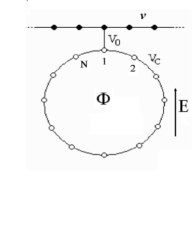
The system under consideration is a quantum ring of $N$ atomic sites connected by tunnel coupling to a quantum wire waveguide, as depicted schematically in Fig. 1. A magnetic flux is assumed to thread the ring and an electric field applied perpendicular to the wire is also considered. The full system is modeled by a single-band tight-binding Hamiltonian within a noninteracting picture, that can be written as

$$H=H_{W}+H_{R}+H_{WR},$$ (1)

with

$$H_{W} = -v\sum_{<i\neq j>}\,(c_{i}^{\dagger}c_{j}+c_{i}c_{j}^{\dagger}),$$

$$H_{R} = \sum_{l=1}^{N}\varepsilon_{l}d_{l}^{\dagger}d_{l}-V_{c}(e^{i2\pi\varphi}\,d_{1}^{\dagger}d_{N}+\mbox{h. c.})$$

$$+ \sum_{l=1}^{N-1}(V_{c}\,d_{l}^{\dagger}d_{l+1}+\mbox{h. c.}),$$

$$H_{WR} = -V_{0}(d_{1}^{\dagger}c_{0}+\mbox{h. c.}),$$ (2)

where $c_{i}^{\dagger}$ and $d_{l}^{\dagger}$ are the creation operators of an electron at site $i$ and $l$ in the wire and the ring, respectively, $v$($V_{c}$) is the corresponding hopping energy in the wire (ring) and $V_{0}$ is the ring-wire tunneling coupling. The site energies of the wire and the ring are set at zero and $\varepsilon_{l}$ respectively. The magnetic flux is measured in terms of the elemental quantum flux $\Phi_{o}=hc/e$ as $\varphi=\Phi/\Phi_{0}$. We adopt the singular gauge for the vector potential associated with the magnetic field, in which all the effects of the field are included explicitly in the hopping energy between the first ($1$) and last ($N$) sites of the ring.singular

The eigenstates of the wire Hamiltonian ($H_{W}$) may be written as

$$\left|k\right\rangle=\sum_{j=-\infty}^{\infty}e^{ikdj}\left|j\right\rangle,$$ (3)

where $d$ is the atomic spacing and $\left|j\right\rangle$ denotes a Wannier state localized at site $j$. The dispersion relation associated with these Bloch states reads $\varepsilon(k)=-2v\cos(kd)$, where the wave vector $k$ is defined within the corresponding first Brillouin zone $[-\pi/d,\pi/d]$.

The stationary states of the complete Hamiltonian (Eq. (1)) may be written as

$$\left|\psi_{k}\right\rangle=\sum_{j=-\infty}^{\infty}a_{j}^{k}\left|j\right\rangle+\sum_{l=1}^{N}b_{l}^{k}\left|l\right\rangle,$$ (4)

where the coefficient $a_{j}^{k}$ ($b_{l}^{k}$) is the probability amplitude to find the electron in the site $j(l)$ of the quantum wire (ring) in the state $k$.

Solving the eigenvalue problem for $H$ one obtains the following linear set of coupled equations

$$\varepsilon a_{j}^{k} = -v(a_{j-1}^{k}+a_{j+1}^{k})-V_{0}b_{1}^{k}\delta_{j0},$$

$$\varepsilon b_{1}^{k} = \varepsilon_{1}b_{1}^{k}-V_{c}e^{i2\pi\varphi}b_{N}^{k}-V_{c}b_{2}^{k}-V_{0}a_{0}^{k},$$

$$\varepsilon b_{l}^{k} = \varepsilon_{l}b_{l}^{k}-V_{c}b_{l-1}^{k}-V_{c}b_{l+1}^{k}\quad\mbox{for $l=2,...,N-1$},$$

$$\varepsilon b_{N}^{k} = \varepsilon_{N}b_{N}^{k}-V_{c}b_{N-1}^{k}-V_{c}e^{-i2\pi\varphi}b_{1}^{k}.$$ (5)

The relationship between the probability amplitudes at the junction is then given by

$$b_{1}^{k}=\frac{-D_{2,N}(\varepsilon)}{\widetilde{D}_{N}(\varepsilon)}V_{0}a_{0}^{k},$$ (6)

where $\widetilde{D}_{N}(\varepsilon)$ $=\det(\varepsilon I-H_{R})$, and $D_{n,m}(\varepsilon)$ is given by

$$D_{n,m}(\varepsilon)=\mbox{det}\left[\begin{array}[]{lllll}\varepsilon-\varepsilon_{n}&V_{c}&0&...&0\\ V_{c}&\varepsilon-\varepsilon_{n+1}&V_{c}&...&0\\ 0&V_{c}&...&...&...\\ ...&...&...&\varepsilon-\varepsilon_{m-1}&V_{c}\\ 0&...&0&V_{c}&\varepsilon-\varepsilon_{m}\end{array}\right].$$ (7)

Following standard methods of quantum waveguide transport, one may calculate the transmission coefficient and obtain the probability amplitudes $a_{j}^{k}$ via an iterative procedure.pedro1 As usual, electrons are described by a plane wave incident from the far left with unit amplitude and a reflection amplitude $r$, and at the far right by a transmission amplitude $t$. For a given transmission amplitude, the associated incident and reflection amplitudes may be determined by matching the iterated function to the proper plane wave at the far left. For $a_{0}^{k}$ one gets

$$a_{0}^{k}=t = \frac{2iv\sin(kd)}{2iv\sin(kd)-V_{0}^{2}D_{2,N}(\varepsilon)/\widetilde{D}_{N}(\varepsilon)}$$ (8)

$$= \frac{\widetilde{D}_{N}(\varepsilon)}{\widetilde{D}_{N}(\varepsilon)+i\Gamma D_{2,N}(\varepsilon)},$$ (9)

where $\Gamma(k)\equiv\Gamma_{0}/\sin(kd)$ , with $\Gamma_{0}=V_{0}^{2}/2v$. The transmission probability is given by $T=\left|t\right|^{2}$.

The linear conductance at the Fermi level is calculated via the one-channel Landauer formula at zero temperature. Actually, the conductance is the experimentally accessible quantity related to the transmission probability $T$,

$$G(\varepsilon)=\frac{2e^{2}}{h}\,T(\varepsilon)=\frac{2e^{2}}{h}\,\frac{\left|\widetilde{D}_{N}(\varepsilon)\right|^{2}}{\left|\widetilde{D}_{N}(\varepsilon)\right|^{2}+\Gamma^{2}\left|D_{2,N}(\varepsilon)\right|^{2}}.$$ (10)

One observes that $G(\varepsilon)$ vanishes when $\widetilde{D}_{N}(\varepsilon)$ is zero, and is equal to $2e^{2}/h$ for null values of $D_{2,N}(\varepsilon)$. One should notice that the zeros of $\widetilde{D}_{N}(\varepsilon)$ correspond to the energy spectrum of the isolate ring. Thus, the energy spectrum of a particular ring configuration may be obtained by measuring the zeros of the conductance.

In the case of a magnetic flux threading the ring, one knows that a persistent current is generated through the circular system. The persistent current density $J$ along the ring, in the energy interval $d\varepsilon$ around $\varepsilon$, is obtained from pedro2

$$J=\frac{2eV_{c}}{\hbar}\,Im(b_{l+1}^{*}b_{l}).$$ (11)

As this quantity does not depend on the site $l$, one may evaluate it between any pair of coupled sites. For simplicity, we choose $l=1$ and $2$. It follows from Eqs. (5) that for a ring of $N$ sites, $b_{2}^{k}$ is given by

$$b_{2}^{k}=V_{0}V_{c}\frac{(D_{3,N}(\varepsilon)+\cos(N\pi)e^{-i2\pi\varphi}V_{c}^{N-2})}{\widetilde{D}_{N}(\varepsilon)}a_{0}^{k},$$ (12)

which together with Eqs. (6), (9) and (11) gives

$$J=-\frac{2ev}{\hbar}\,\sin(2\pi\varphi)\frac{\cos(N\pi)\Gamma_{0}V_{c}^{N}D_{2,N}(\varepsilon)}{\left|\widetilde{D}_{N}(\varepsilon)\right|^{2}+\Gamma^{2}\left|D_{2,N}(\varepsilon)\right|^{2}}.$$ (13)

It is worth noting that when $D_{2,N}=0$ and $\widetilde{D}_{N}\neq 0$, the transmission is perfect ($G=2e^{2}/h$) and the persistent current density vanishes. On the other hand, when $\widetilde{D}_{N}=0$, the linear conductance vanishes and the persistent current density oscillates regularly with the magnetic flux with period $\Phi_{0}$.

III Zero electric field

Let us introduce the dimensionless conductance $g=G/(2e^{2}/h)$ and persistent current density $j=J/(2ev/\hbar)$. For zero electric field, we assume here the particular case of a uniform ring where the ring site energies are $\varepsilon_{l}=\varepsilon_{o}=0$ (for $l=1,...,N$). The dimensionless conductance $g(\varepsilon)$ can be written in a compact form, which depends explicitly on the size of the ring,

Figure 2: Dimensionless conductance as a function of $\theta$ ($\theta=\arccos(\varepsilon/2V_{c})$), for rings composed of (a) 5, (b) 6, (c) 11, and (d) 12 atomic sites) and for a magnetic flux equal to 0.3.

Figure 3: Dimensionless conductance as a function of the magnetic flux $\varphi=\Phi/\Phi_{o}$ for rings composed of (a) 11, and (b) 12 atomic sites.

$$g(\varepsilon)=\frac{1}{1+h(\varepsilon)},$$ (14)

where

$$h(\varepsilon)=\frac{(\prod\limits_{i=1}^{N-1}[\varepsilon-2V_{c}\cos(\pi i/N)])^{2}\Gamma^{2}}{(\prod\limits_{i=0}^{N-1}\{\varepsilon-2V_{c}\cos[2\pi(i+\varphi)/N]\})^{2}}$$ (15)

The occurrence of resonances ($g(\varepsilon)=1$) are then expected at $\varepsilon=2V_{c}\cos(\pi i/N)$ ($i=1,...,N-1$) and are independent of the magnetic flux, whereas antiresonances (that is, $g(\varepsilon)=0$) take place at energies $\varepsilon=2V_{c}\cos[2\pi(i+\varphi)/N]$ ($i=0,...,N-1$). Introducing the energy parameter defined by $\theta=\arccos(\frac{1}{2}\varepsilon/V_{c})$, $h(\varepsilon)$ may be written (see details in the Appendix) as

$$h(\varepsilon)=\frac{(\Gamma/2V_{c})^{2}\sin(N\theta)^{2}}{\sin(\theta)^{2}[\cos(N\theta)-\cos(N\pi)\cos(2\pi\varphi)]^{2}}.$$ (16)

Figure 4: Dimensionless current density as a function of the Fermi energy for rings with N$=11$ (solid curve) and N$=12$ (dot line) atomic sites, and for a magnetic flux equal to $0.3$.

Results for the conductance as a function of $\theta$ are shown in Figure 2 for rings of different sizes and considering a magnetic flux $\varphi=0.3$ and $\Gamma_{0}=V_{c}$. The conductance clearly exhibits an oscillating pattern of resonances and antiresonances for particular energies which depend on the number of sites in the ring. As mentioned above, the corresponding antiresonant energies give us the energy spectrum of the ring. The quantum wire conductance dependence on the magnetic flux is explicitly shown in Figure 3 for two values of $N$ ($N=11$ and 12), considering a Fermi energy equal to $0.3V_{c}$. The oscillatory period of a quantum of flux is found, independent of the ring order, as expected from the analytical expression for the conductance [Eq. (16)]. This behavior is compatible with the results found by Shi and Gu for the case of one ring side-attached to leads.gu Let us now calculate the persistent current density. For a regular ring this reduces to

$$j(\varepsilon)=\frac{(\Gamma_{0}/2V_{c})\cos(N\pi)\sin(N\theta)\sin(\theta)\sin(2\pi\varphi)}{\sin^{2}(\theta)[\cos(N\theta)-\cos(N\pi)\cos(2\pi\varphi)]^{2}+(\Gamma/2V_{c})^{2}\sin(N\theta)^{2}}.$$ (17)

One clearly notices that $j$ is an oscillating function of the Fermi energy ($\theta$) and of the magnetic flux ($\varphi$). Moreover, in the limit $\Gamma\rightarrow 0$ the current density exhibits a delta function behavior in the energies of the isolated ring (this limit correspond to the disconnected ring).

Figure 5: Dimensionless current density as a function of the magnetic flux for a Fermi energy equal to 0.1$V_{c}$ and for (a) $N=11$ and (b) $N=12$.

It is straightforward to show from Eq. (16) that when the Fermi energy is pinned at zero ($\theta=\pi/2$), the dimensionless conductance $g$ reduces to

$$g = \frac{\cos(2\pi\varphi)^{2}}{\cos(2\pi\varphi)^{2}+\left(\Gamma/2V_{c}\right)^{2}},\quad N\text{ odd}$$

$$g\, = \,1,\quad N\text{ even},$$ (18)

and the corresponding persistent current density is

$$j = \frac{(\Gamma_{0}/2V_{c})\sin(2\pi\varphi)}{\cos(2\pi\varphi)^{2}+\left(\Gamma/2V_{c}\right)^{2}},\quad N\text{ odd}$$

$$j = \,0,\quad N\text{ even}.$$ (19)

Figure 6: Dimensionless conductance as a function of the Fermi energy, for a ring with N$=11$, a magnetic flux $\varphi=0.3$, and for distinct electric field intensities, (a) $E^{*}=0.05$, and (b) $E^{*}=0.15$

Notice that for a uniform ring of even $N$, perfect transmission takes place ($g=1$) and the persistent current density vanishes ($j=0$) for any value of the magnetic flux. The transmission is perfect in this case because for this energy the electron does not enter the ring (in fact, it can be shown that its phase remains unaltered), and therefore the magnetic flux does not play any role in the conductance. This also explains that the persistent current density is zero. For $N$ odd, the transmission and the persistent current density oscillate regularly with the magnetic flux.

The persistent current density as a function of the dimensionless energy $\varepsilon^{*}$ ($\varepsilon^{*}=\varepsilon/2V_{c}$) is depicted in Figure 4 for two ring configurations ($N=11$ and $12$), for a magnetic flux $\varphi=0.3$. The expected oscillatory behavior with the energy is clearly evidenced, as well as the dependence on the magnetic flux, as shown in Figure 5 for the fixed energy $\varepsilon^{*}=0.1$, and for both an odd and an even ring number configuration.

Figure 7: Electronic spectrum of an 11 sites ring as a function of a) the electric field strength, for a magnetic flux of $\varphi=0.3$, b) the magnetic flux, for an electric field strength of $E^{*}=0.1$. The energy is in units of $2V_{c}$.

IV Electric field effects

Within the tight-binding approximation, and assuming an in-plane ring electric field perpendicular to the wire, the dependence of the site energy on the field may be expressed as $\varepsilon_{l}=(eEdN/2\pi)\cos(2\pi(l-1)/N)=(eV_{c})(E^{*}N/2\pi)\cos(2\pi(l-1)/N)$, where we define the dimensionless electric field strength $E^{*}=Ed/V_{c}$. The determinants $\widetilde{D}_{N}(\varepsilon)$ and $D_{1,N}(\varepsilon)$ are now calculated iteratively (see details in the Appendix). Figure 6 shows the dimensionless conductance as a function of the Fermi energy, for a ring with $N=11$ sites, magnetic flux $\varphi=0.3$, and two electric field values. The main effects of the electric field is to shift and squeeze the resonances and antiresonances of the linear conductance.

The energy spectrum of an isolated ring ($N=11$) in the presence of both magnetic and electric field is also analyzed. The dependence of the spectrum on the electric field energy is displayed in Figure (7-a), for $\varphi=0.3$, whereas Figure (7-b) shows the explicit dependence on the magnetic flux for an electric field $E^{*}=0.1$. One of the main effects of the electric field is the suppression of the Aharonov-Bohm oscillations in the edges of the energy spectra, being as the lowest and highest-lying energy levels are almost independent on the magnetic flux. For energies in the center of the energy spectrum new oscillations with the quantum-flux period are developed. Quite similar results were found before for the case of a finite-width semiconducting quantum ring.pupi

Figure 8: Dimensionless current density in $N=11$ sites ring as a function of magnetic flux for different values of electric field, $E^{*}=0.0$ (solid line), $E^{*}=0.1$ (dash line), $E^{*}=0.2$ (dot line) and $E=0.3^{*}$ (dash-dot line)

As expected, the current density is also affected by the electric field. Figure 8 shows the dimensionless current density as a function of the magnetic flux for different values of the electric field. As we can appreciate, the persistent current density decreases with the electric field strength. It is shown more clearly in Figure 9. This figure shows the normalized current density $j/j_{0}$ associated with the lowest level of the energy spectrum as a function of the electric field strength for for a fixed magnetic flux ($j_{0}$ current density at zero magnetic flux). The current density decays exponentially with the electric field strength. This way, the electric field can be used to control the persistent current in quantum rings.

Figure 9: Dimensionless current density in $N=11$ sites ring as a function of electric field strength for fixed magnetic flux $\varphi=0.3$ (solid line) and $\varphi=0.4$ (dash line).

V Summary

The conductance and the persistent current density, at zero temperature, of a side ring attached to a quantum wire was investigated. We found that the system develops an oscillating band with antiresonances and resonances arising from the hybridization of the quasibound levels of the ring and the coupling to the quantum wire. The positions of the antiresonances correspond exactly to the electronic spectrum of the isolated ring. For a uniform ring we found that the system shows odd-even parity in the conductance and also in the persistent current density. Namely, when the Fermi energy is pinned at zero, if the number of sites in the ring is even, perfect transmission takes place and the persistent current density vanishes for any value of the magnetic field. When this number is odd, the transmission and current density oscillate periodically with the magnetic flux. The effects of an in-plane electric field were also studied. We found that this shifts the electronic spectrum and damps the amplitude of the persistent current density. These features may be used to control externally the energy spectra and the amplitude of the persistent current.

APPENDIX

We present here the properties of the determinant $D_{n,m}(\varepsilon)$ which is defined by Eq. (5). It is easy to show that the following recurrence relation is valid

$$D_{n,m}=(\varepsilon-\varepsilon_{n})D_{n+1,m}-V_{c}^{2}D_{n+2,m},$$ (20)

$$n=1,2...,m,m=3,4,...$$

with $D_{m,m}=\varepsilon-\varepsilon_{m}$ and $D_{m-1,m}$ $=(\varepsilon-\varepsilon_{m-1})(\varepsilon-\varepsilon_{m})-V_{c}^{2}$. Mainly for a uniform case $\varepsilon_{m}=0$ for all $m^{{}^{\prime}}s$, the expression for $D_{n,m}\equiv D_{n}$ can be found in a explicit form. In fact, $D_{n}(\varepsilon)$ is related with the type-II Chebyshev polynomial,

$$D_{n}(\varepsilon)=V_{c}^{n}U_{n}(\frac{1}{2}\varepsilon/V_{c}).$$ (21)

Then it is straightforward to show that

$$D_{n}=V_{c}^{n}\frac{\sin((n+1)\theta)}{\sin\theta}=\prod\limits_{i=1}^{n}(\varepsilon-2V_{c}\cos(\pi i/(n+1))).$$ (22)

The determinant $\widetilde{D}_{N}$ can be written in function of the determinant $D_{n,m}$ as

$$\widetilde{D}_{N} = (\varepsilon-\varepsilon_{1})D_{2,N}-V_{c}^{2}(D_{3,N}+D_{2,N-1})$$ (23)

$$- 2V_{c}^{N}\cos(N\pi)\cos(2\pi\varphi).$$

In the particular case when $\varepsilon_{m}=0$ for all $m^{{}^{\prime}}s$, the expression for $\widetilde{D}_{N}$ can be written in terms of the eigenvalues of $H_{N}$ $(\varepsilon_{i}=2V_{c}\cos(2\pi(i+\varphi)/N)).$

$$\widetilde{D}_{N}=\prod\limits_{i=1}^{N}(\varepsilon-2V_{c}\cos(2\pi(i+\varphi)/N)).$$ (24)

Additionally, from Eq.(21) we can write the determinant $\widetilde{D}_{N}$ as a function of $\theta$,

$$\widetilde{D}_{N} = \varepsilon D_{N-1}-2V_{c}^{2}D_{N-2}-V_{c}^{N}\cos(N\pi)\cos(2\pi\varphi)$$ (25)

$$= 2V_{c}^{N}[\cos(N\theta)-\cos(N\pi)\cos(2\pi\varphi)].$$

References

- (1) V. Chandrasekhar, R.A. Webb, M.J. Brady, M.B. Ketchen, W.J. Gallagher and A. Kleinsasser, Phys. Rev. Lett. 67 3578 (1991).
- (2) D. Mailly, C. Chapelier and A. Benoit, Phys. Rev Lett. 70 2020 (1993).
- (3) U. F. Keyser, C. Fühner, S. Borck and R. J. Haug, Semm. Sc. and Tech. 17, L22 (2002).
- (4) A. Lorke, R. J. Luyken, A. O. Govorov, Jürg P. Kotthaus, J. M. García, P. M. Petroff, Phys. Rev. Lett. 84 2223 (2000).
- (5) A. Fuhrer, S. Lüscher, T. Ihn, T. Heinzel, K. Ensslin, W. Wegscheiner, M. Bichler, Nature 413 385 (2001).
- (6) A.I. Yanson, G. Rubio-Bollinger, H. E. van den Brom, N. Agra¨, and J.M. van Ruitenbeek, Nature (London),395, 780 (1998).
- (7) F.R. Waugh, M.J. Berry, C.H. Crouch, C. Livermore, D.J. Mar, and R.M. Westervelt, K.L. Campman and A.C. Gossard, Phys. Rev. B. 53 1413 (1996).
- (8) Midori Kawamura, Neelima Paul, Vasily Cherepanov, and Bert Voigtlanänder, Phys. Rev. Lett. 91, 096102 (2003).
- (9) R.H.M. Smit, C. Untiedt, G. Rubio-Bollinger, R.C. Segers, and J.M. van Ruitenbeek, Phys. Rev. Lett. 91, 076805 (2003).
- (10) Z.Y. Zeng and F.Claro, Phys. Rev. B 65, 193405 (2002).
- (11) T.S. Kim and S. Hershfield, Phys. Rev. B. 65, 214526 (2002).
- (12) H.-S. Sim, H.-W. Lee, and K.J. Chang, Phys. Rev. Lett. 87, 096803 (2001).
- (13) M. Büttiker, Phys. Rev. B 32 1846 (1985).
- (14) D. Takai and K. Ohta, J. Phys. Cond. Matt. 6, 5485 (1994); ibid Phys. Rev. B 48, 14318 (1993).
- (15) A. M. Jayannavar and P. Singha Deo, Phys. Rev. B 49, 13685 (1994).
- (16) Ji-Rong Shi and Ben-Yuan Gu, Phys. Rev. B 55, 4703 (1997).
- (17) Jorge L. D’Amato, Horario M. Pastawski, and Juan F. Weisz, Phys. Rev. B 39, 3554 (1989).
- (18) Youyan Liu and P.M. Hui, Phys. Rev. B 57,12994 (1998).
- (19) Ho-Fai Cheung and Eberhard K. Riedel, Phys. Rev. B 40, 9498 (1989).
- (20) Yan Chen, Shi-Jie Xiong, S. N. Evangelou, Phys. Rev. B 56, 4778 (1997).
- (21) J. P. Carini, K. A. Muttalib, and S. R. Nagel, Phys. Rev. Lett. 53, 102 (1984).
- (22) P. A. Orellana, F. Dominguez-Adame, I. Gomez, and M. L. Ladrón de Guevara, Phys. Rev. B 67, 085321 (2003).
- (23) Pedro A. Orellana, G.A. Lara and Enrique V. Anda, Phys. Rev. B 65, 155317 (2002).
- (24) Z. Barticevic, G. Fuster and M. Pacheco, Phys. Rev. B 65 193307 (2002).