Lévy statistics and anomalous transport in quantum dot arrays

Abstract

A novel model of transport is proposed to explain power law current transients and memory phenomena observed in partially ordered arrays of semiconducting nanocrystals. The model describes electron transport by a stationary Lévy process of transmission events and thereby requires no time dependence of system properties. The waiting time distribution with a characteristic long tail gives rise to a nonstationary response in the presence of a voltage pulse. We report on noise measurements that agree well with the predicted non–Poissonian fluctuations in current, and discuss possible mechanisms leading to this behavior.

I Introduction

Arrays of semiconductor nanocrystals Bawendi (quantum dot arrays, or QDAs) are of great interest for both the fundamental solid state physics and applications. Self–assembled QDAs is one of the simplest examples of macroscopic complex systems built from the “artificial atoms” with pre–designed properties at the nanoscale. From the basic research perspective, these arrays are compelling since one can control the Hamiltonian by design. In particular, they open new possibilities to create systems with desirable unconventional transport properties. Charge and spin transport in QDAs could lead to applications in spintronics and quantum computation. spintronics

Despite the progress in synthesis and fabrication of nanocrystal arrays, the nature of electronic transport in them is still poorly understood. Like other problems involving long–range Coulomb interactions in disordered systems, this problem appears to be challenging. Proposed theoretical models include mapping onto the problem of interface dynamics,Wingreen onto a frustrated antiferromagnetic spin model with long range interactions,Novikov01 as well as recent generalizations ZhangShklovskii of the variable range hopping scenario.conventional

In the present work we attempt to explain the recently observedqdots-transport ; nicole transient power–law decay of current

$$I(t)=I_{0}\;t^{-\alpha}\,,\quad 0<\alpha<1$$ (1)

as a response to a step in large bias voltage applied across the array. The exponent $\alpha$ depends on temperature, dot size, capping layer, bias voltage and gate oxide thickness in a systematic way.qdots-transport ; nicole It is interesting that the observed $\alpha$ is less than one in all samples. The condition $\alpha<1$ ensures that (1) is a true current from source to drain, rather than a displacement current, since the net charge corresponding to (1) diverges with time, $Q=\int I(t)dt\to\infty$. At the same time, remarkably, the transient transport also possesses memory. Namely, if the bias is turned off for $t_{1}<t<t_{2}$, then the current measured as a function of the time $\tilde{t}=t-t_{2}$ after reapplying the voltage follows the dependence (1), albeit with a reduced amplitude $\tilde{I_{0}}<I_{0}$: $I(t)=\tilde{I_{0}}(t-t_{2})^{-\alpha}$. The amplitude is restored to its initial value, $\tilde{I_{0}}\to{I_{0}}$, by increasing the off interval $t_{2}-t_{1}$, by annealing at elevated temperature, or by applying a reverse bias or band gap light between $t_{1}$ and $t_{2}$. qdots-transport ; nicole ; ginger

The behavior (1) is observed in partially ordered multi–layered arrays of II–VI semiconductor nanocrystals. Each nanocrystal is capped with $\sim$1 nm coating, so that electrons must tunnel to move between neighboring sites. Although the transient response (1) has been recorded by a number of groups,qdots-transport ; ginger ; nicole ; sionnest-science ; sionnest its origin remains a mystery. In many systems the transient (1) comprises the dominant contribution to transport, while the ohmic conductivity is quite small.Marija-AFM Understanding the nature of the time–dependent response (1) may shed light on the dynamics of carriers in such systems.

It has been suggested earlier that the observed time–dependent current could be a result of time dependence of the state of the system. The latter could arise either because of charge flow jamming, due to trapping of electrons blocking further charge injection from the contact,ginger or because of the Coulomb glass behavior of the electrons distributed over QDAs. qdots-transport However, it seems that such a scenario would require an unlikely fine–tuning as a function of time. Namely, the system’s properties would have to adjust in a coherent fashion over many hours to yield well–reproducible power laws in current, observed over at least five orders of magnitude in time in a broad variety of samples.

The purpose of this work is to suggest an alternative point of view on transport in QDAs, which does not require time–varying system’s properties. We propose a model, based on the Lévy statistics of waiting times between charge transmission events, in which the system remains stationary in statistical sense, but nonetheless exhibits a transient response. The model is corroborated by the measurements of the spectrum of time–dependent current fluctuations in CdSe QDAs, and a good agreement is demonstrated.

This paper is organized as follows. We begin with introducing a phenomenological model of transport which yields the response (1). We consider manifestations of this transport mechanism in the noise spectrum, and report the results of noise measurements. Finally, we briefly discuss possible microscopic mechanisms that could be consistent with our transport model.

II Model of transport

The main idea of our approach is that current (1) can arise as a result of a stationary stochastic process. Our model involves $N\gg 1$ identical independent conducting channels arranged in parallel. (This accounts for the typical sample’s aspect ratio $\sim 10^{3}\,\mu$m : $1\,\mu$m.) Each channel is almost always closed, and opens up at random for a short interval $\tau_{0}$ to conduct a current pulse that corresponds to a unit transmitted charge, as schematically shown in the lower inset of Fig. 1. We further assume that the intervals between subsequent transmissions are uncorrelated, making the process completely characterized by the waiting time distribution (WTD) of intervals between successive pulses.

In particular, we will be interested in WTD $p(\tau)$ with a broad tail at long times. In order to model the power law decay of the current transient, here we consider a special form of WTD with a long tail of the Lévy type:

$$p(\tau\gg\tau_{0})\simeq\frac{a}{\tau^{1+\mu}}\,,\quad 0<\mu<1\,,$$ (2)

with $\tau_{0}$ a miscroscopic time scale. Note that all moments of $p(\tau)$ diverge. The behavior of the WTD at short times, $p(\tau\sim\tau_{0})$, is not of interest, since it does not affect the long time dynamics.

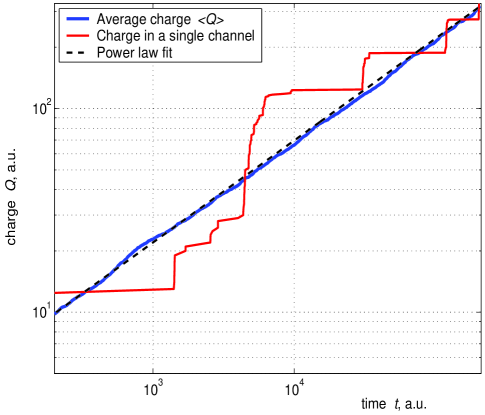
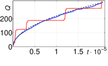
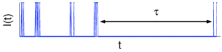
Figure 1: Time dependence of the net transmitted charge $Q(t)$ in a single channel (red line) and charge $\left<Q(t)\right>$ averaged over $N=100$ channels (blue line) simulated using WTD of the form (2) with $\mu=0.5$ (double log scale). Dashed line is a power law $Q\propto t^{\mu}$. Upper inset: The same plot in the linear scale. The large charge noise in a single channel is due to the lack of self-averaging for a wide-tail WTD. Lower inset: Current in a single channel with a wide distribution of waiting times (schematic). Short packets of current pulses are separated by very long waiting times $\tau\gg\tau_{0}$.

As shown in Appendix A, WTD of the form (2) indeed yields the power law decay (1) for the mean value of the current in a single channel with $\alpha=1-\mu$ and $I_{0}=\mu\sin\pi\mu/\pi a$. Qualitatively, the decrease in current with time can be understood as follows. The mean value of the waiting time for the process with WTD (2) is infinite. Thus, for a stochastic process governed by the WTD (2) which started infinitely early in the past, the observed value of the current would be zero. Turning the bias on at $t=0$ sets the clock for the process. In this case, for the measurement interval $t$, only the waiting times $\tau\leq t$ can occur, as illustrated by the simulation shown in Fig. 1 (note the double log scale). Observing the current over a larger time period effectively increases the chances for a channel to be closed for a longer time interval, which results in the decay in the average current, the latter approaching zero at $t\to\infty$. We note that in this transport model the system’s parameters characterizing the distribution (2) are time independent. Hence the process is stationary, i.e. each charge transmission event occurs after a delay time $\tau$ described by the distribution $p(\tau)$ independent of the total time $t$ passed after the beginning of the measurement.

Continuous time random walks with the Lévy WTDs often arise in the systems characterized by wide distributions of time scales.Bouchaud In the semiconductor physics the Lévy processes have been extensively studied in the context of the dispersive transport, e.g. in amorphous semiconductors. dispersive-transport A simple example is a system of electrons moving between charge traps. Its dynamics depends on energy $\epsilon$ via an activation exponential, $\tau=\tau_{0}\,e^{\beta\epsilon}$, where $\beta$ is the inverse temperature. For the distribution of the energies $\epsilon$ described by the density of states of exponential form, $\nu(\epsilon)=\nu_{0}e^{-b\epsilon}$, one obtains $p(\tau)$ of the power law form (2) with exponent $\mu=b/\beta$ and $a=\nu_{0}\,\tau_{0}^{\mu}/\beta$.

The probability distribution (2) leads to an unusual behavior which is the subject of the theory of Lévy flights. Levy-flights The main characteristic of the Lévy statisticsLevy-flights ; Bouchaud is the violation of the central limit theorem. To illustrate this unconventional behavior, let us recall what happens in a Poissonian channel characterized by the finite mean waiting time $\bar{\tau}$. The mean value of the transmitted charge $Q$ grows linearly with time, $\left<Q\right>=t/\bar{\tau}$, corresponding to a constant current. The variance of the charge is proportional to the mean, $\left<\!\left<Q^{2}\right>\!\right>=\frac{1}{2}\left<Q\right>$, in other words the relative charge fluctuation decreases, $\left<\!\left<Q^{2}\right>\!\right>^{1/2}/\left<Q\right>\propto t^{-1/2}$, in accord with the central limit theorem. In contrast, in the case of the distribution (2), the mean transmitted charge increases sublinearly as $\left<Q\right>\sim t^{\mu}$, whereas its variance is proportional to the square of the mean, $\left<\!\left<Q^{2}\right>\!\right>\propto\left<Q\right>^{2}$ (see Appendix A). Since relative charge fluctuation does not decrease with time, transport in a single channel is dominated by large fluctuations of waiting times (see Fig. 1).

Although in our model any given channel lacks self–averaging, the charge summed over $N\gg 1$ independent parallel channels averages to a smooth power law, Fig. 1, with fluctuations reduced by a factor of $N^{-1/2}$. For the typical sample geometry used in our experiments, consisting of ca. 50 layers, each layer of $1.6\cdot 10^{5}$ dots wide and 200 dots across, one expects large effective $N$ and small current fluctuations, as in Refs. qdots-transport, ; nicole, .

Also, as a check of robustness of this scenario with respect to spatially varying system properties, we considered parallel non–identical channels, characterized by non–equal values of $\mu$. We found that the average current obtained from such a model is approximately described by a power law of the form (1). We performed a simulation with $N=100$ channels, with the exponents of different channels drawn from a flat distribution, $0.45<\mu<0.55$. In this case, the transmitted charge time dependence was found to be numerically very close to that given in Fig. 1 with $\mu=0.5$.

III Memory Effects

Memory effects originate in our transport model in the manner analogous to aging in the Lévy systems.barkai'03 Because of large typical waiting times $\tau\gg\tau_{0}$, any given channel is most likely found in a non–conducting state when the voltage is turned off at $t=t_{1}$. In addition, we assume that, due to gradual time variation of channel parameters, taken to be very slow in this discussion, the channel state is likely to remain unchanged by the time the voltage is turned back on at $t=t_{2}>t_{1}$. In this case the channel conducts current as if the voltage has been on all the time. However, due to the aforementioned time variation of system parameters, there is a chance that the channel changes its state (resets) while the voltage is turned off during $t_{1}<t<t_{2}$. This reset probability $w_{12}\equiv w(t_{2}-t_{1})$, as a function of the off time $t_{2}-t_{1}$, is growing monotonically: $w(\tau_{0})\approx 0$, $w(\infty)=1$. As a simple model of this behavior, one can consider a Poisson process,

$$w(\tau)=1-e^{-\gamma t}$$

with the rate parameter $\gamma$ characterizing the reset probability.

The current at $t=t_{2}$ as a function of the shifted time $\tilde{t}=t-t_{2}$, obtained by averaging over $N\gg 1$ channels, is given by

$$I(\,\tilde{t}\,)=(1-w_{12})I_{0}\,(\tilde{t}+t_{2})^{-\alpha}\,+\,w_{12}I_{0}\,\tilde{t}^{-\alpha}\,.$$ (3)

Here we assume the reset of different channels to be independent and uncorrelated. The function $I(\tilde{t})$ has a singular part at $\tilde{t}\approx 0$ (the second term of Eq.(3)) with the amplitude $\tilde{I}_{0}=w_{12}I_{0}$ reduced compared to $I_{0}$ by the reset probability $w_{12}<1$. Thus at $\tilde{t}\ll t_{2}-t_{1}$ the first (regular) term in Eq. (3) is negligible compared to the second term. The current (3) is dominated by the latter, resulting in suppression of the measured transient current part which is singular at $t\approx t_{2}$.

We note that the described reset process, while leading to suppression of the singular part of the current, is accompanied by an overall enhancement of the total current (3), as compared to the current (1) at time $t$ in the absense of resetting. This prediction indeed agrees with our observations. We have verified that the reset probability $w_{12}=\tilde{I}_{0}/I_{0}$ is indeed a monotonic function of the time interval when the voltage is turned off. For waiting times from $10\,{\rm s}$ to $10^{4}\,{\rm s}$ in between $100\,{\rm s}$ long transients, we measure $0.65<w_{12}<0.85$; $w_{12}\to 1$ when applying a reverse bias, exposing the dots to the band gap light or waiting for longer times.

IV Noise frequency spectrum

The model described above, which is consistent with previously reported transport measurements, can be independently verified with the help of noise measurements. Here we consider the statistics of current fluctuations and formulate a prediction of the model based on the Lévy process (2).

The unconventional fluctuations exhibited by the Lévy process, discussed in Section II, manifest themselves in noise as follows. Consider the time-dependent current in a single channel, described in Section II, recorded during a long time interval $T\gg\tau_{0}$:

$$I(t)=\sum_{n=1,2,...}\delta(t-t_{n})\,,\quad 0<t<T\,.$$ (4)

The intervals $\tau_{n}=t_{n}-t_{n-1}$, $n=1,2,...$, $t_{0}\equiv 0$, are independent random variables distributed according to the WTD of the form (2). The fluctuations of current are defined in terms of the Fourier harmonics

$$I_{\omega}=\int_{0}^{T}e^{i\omega t}I(t)dt\,.$$ (5)

Here we consider the noise power spectrum

$$S(\omega)=\left<\left<I_{-\omega}I_{\omega}\right>\right>=\left<I_{-\omega}I_{\omega}\right>-\left<I_{-\omega}\right>\left<I_{\omega}\right>\,.$$ (6)

In Appendix A we show that the distribution (2) leads to the non–Poissonian spectrum

$$S(\omega)\propto\cases{T^{2\mu}\,,&$\omega T\ll 1$ ,\cr T^{\mu}\omega^{-\mu}\,,&$\omega T\gg 1$ .}$$ (7)

Here the low frequency part of (7) with $\omega T\ll 1$ corresponds to the fluctuation $\left<\!\left<Q^{2}\right>\!\right>$ of the net transmitted charge. Due to the relation $\left<\!\left<Q^{2}\right>\!\right>\propto\left<Q(T)\right>^{2}$ [Eq. (24)] between the first two moments of the Lévy process, which violates the central limit theorem, the quantity $S(\omega T\ll 1)$ is proportional to the square of the mean transmitted charge $Q(T)\propto T^{\mu}$.

Experimentally, however, it is more convenient to deal with $S(\omega)$ at finite frequency $\omega T\gg 1$. Eq. (7) predicts a characteristic power law spectrum for this quantity. We note that for $\omega T\gg 1$, the Lévy process (2) yields identical power laws for the noise spectrum (7) and for the average current, $\left<I_{\omega}\right>\sim\omega^{-\mu}$. Moreover, the relationship

$$\left<\left<I_{-\omega}I_{\omega}\right>\right>\propto\left<I_{\omega}\right>\propto\omega^{-\mu}\,,\quad\omega T\gg 1\,,$$ (8)

is robust with respect to averaging over $N$ independent channels, since for such averaging the central limit theorem holds. An experimental test of the proportionality relationship (8) between the frequency spectra of current and noise will be discussed below.

V Noise measurements

Here we briefly describe the experiments performed to obtain the data on noise frequency spectrum in QDAs. The QDAs were produced as described in Ref.qdots-transport, by self-assembly of nearly identical CdSe nanocrystals, 3 nm in diameter, capped with trioctylphosphine oxide, an organic molecule about 1 nm long. A film of about 200 nm thick of the nanocrystals was deposited on oxidized, degenerately doped Si wafers with oxide thickness $\approx$ 200 nm. The experimental setup was similar to that utilized in Ref. qdots-transport, . Gold electrodes, fabricated on the surface before deposition of the QDA, consist of bars 800$\mu$m long with separation of 2$\mu$m. The sample was annealed at 300 C in vacuum inside the cryostat prior to the electrical measurements. Annealing reduces the distance between the nanocrystals and enhances electron tunneling.qdots-transport

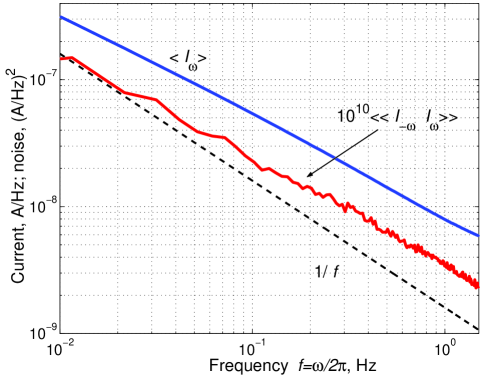
Figure 2: Measured mean current and noise spectrum, with averaging performed over 50 current transients on the same sample. The current Fourier harmonic mean $\left<I_{\omega}\right>$ [Eq. (5)] and variance $\left<\left<I_{-\omega}I_{\omega}\right>\right>$ [Eq. (6)] are shown. Both the current and the noise are described by power law $\omega^{-\mu}$ with the same $\mu\approx 0.72$. The $1/f$ dependence is shown for comparison (see text).

To measure the noise, we have recorded 200 current transients each $t=100$ s long. Measurements have been made on a single sample continuously stored in vacuum, inside of a vacuum cryostat in the dark at $77$ K. Each current transient was recorded for 100 s with a negative bias of $-90$ V. These periods of negative bias were separated from each other by a sequence of zero bias for 10 s, reverse pulse of $+90$ V for 100 s, and zero bias for 10 s, to eliminate the memory effects.qdots-transport We checked that current fluctuations for a substrate without the QDA were several orders of magnitude smaller than with the QDA.

At the beginning of our measurement the current transients were changing from one to the next because of the memory effect described above. Since an error in the average current can yield an error of order $\left<I_{\omega}\right>^{2}\propto\omega^{-2\mu}$ which may affect the measured noise spectrum power law, we discarded the first 150 transients. The noise (Fig. 2) was then deduced from the remaining 50 transients. To further compensate for residual memory effects, each transient was multiplied by a factor $\approx 1$ to have the same net integrated charge. This eliminated the zero frequency contribution to the noise.

Figure 2 shows the measured noise spectrum and the average current measured simultaneously. Both quantities have a power law behavior with nearly identical exponent values $\mu\approx 0.72$ for $\omega t\gg 1$, $t=100$ s. With relative $\sim 3-10\%$ deviations of the noise from the $\omega^{-\mu}$ law, the measured noise spectrum is clearly distinct from the $1/f$ noise typically found at low frequencies. For comparison, in Fig. 2 we draw the $1/f$ dependence, offset so that it coincides with the noise data at the lowest frequency. The discrepancy with the measured noise at the highest frequency by more than a factor of two indicates that the observations are not explained by the $1/f$ noise model.

One may question whether the observed colored noise, instead of being a consequence of the Lévy process, could result from interplay of the intrinsic $1/f$ noise and the time-dependent current decaying according to (1). In this case the fluctuations would be proportional to the current itself:

$$I(t)=\left<I(t)\right>(1+s(t))\,,\quad\left<s(t)s(t^{\prime})\right>\equiv\Gamma(t-t^{\prime})\,,$$ (9)

where $\Gamma_{\omega}\propto\omega^{-\eta}$, $\eta\simeq 1$ for the $1/f$ noise. This would yield the current fluctuation spectrum of the form

$$\left<\!\left<I_{-\omega}I_{\omega}\right>\!\right>=\int|\left<I_{\omega^{\prime}}\right>|^{2}\Gamma_{\omega^{\prime}-\omega}\frac{d\omega^{\prime}}{2\pi}\,.$$ (10)

When $\mu>1/2$, the integral is dominated by the $(\omega^{\prime})^{-2\mu}$ singularity, which effectively sets $\omega^{\prime}=0$, giving rise to the $1/\omega$ behavior. Physically this happens because the current (1) for $\alpha<1/2$ decays slowly enough so that all the harmonics of the $1/f$ noise have time to fully play out.

Conversely, in a system with $\mu<1/2$, the noise $\propto\omega^{-2\mu}$ may be indistinguishable from the errors in determining average current described above. For the consistency check of our model it is important that for our sample the observed current transient power law exponent fulfills $\mu>0.5$. The observation of the $\omega^{-\mu}$ noise indicates that transport is not dominated by the intrinsic $1/f$ noise. Instead, we conclude that the noise measurement agrees with the proposed transport model based on Lévy statistics of transmission events.

VI Discussion

Based on the noise measurements we can estimate the effective number $N$ of conduction channels introduced in Section II. Since both the measured current $\left<I_{\omega}\right>$ and noise $S(\omega)$ are proportional to $N$, the noise-to-current ratio $r(\omega)\equiv S(\omega)/\left<I_{\omega}\right>$ is a characteristic of a single channel. The model calculation for the latter [Appendix A] shows that at large frequency $\omega t\gg 1$ the noise-to-current ratio is frequency independent and proportional to the net charge $Q(t)$ transmitted through the channel during the time $t$ of measurement, $r(\omega t\gg 1)\sim Q(t)$ [Eq. (25)]. From Fig. 2 we find that the measured $r(\omega)$ is indeed frequency independent for $\omega t\gg 1$, and is of the order $r\approx 10^{-10}\,{\rm A}/{\rm Hz}$. [Averaging over 50 transients does not affect $r(\omega)$.] The effective number of channels is then estimated as the ratio of the measured net transmitted charge to that in a single channel, $N\sim\left<I_{\omega=0}\right>/r\sim 10^{4}$. This large number of independent channels is consistent with the sample geometry (aspect ratio $\sim 10^{3}$ and ca. 50 layers of dots).

How can the long waiting times with a distribution of Lévy form (2) arise microscopically? While presently there is no fully satisfactory answer to this question, one can make several observations. First, to rationalize a wide distribution of time scales such as (2), we suppose that the charge hops between neighboring dots are strongly constrained. The simplest constraint to imagine is the lack of energy relaxation (possibly due to a small number of available phonon states) that arises if the on–site energies of electrons on different dots are widely distributed. This is consistent with the absence of ohmic contribution to the conductivity in our QDA. The energy relaxation constraint then allows charge hops only between the aligned energy levels of the dots.

Next, the WTD (2) with a long tail can be explained if the energy levels strongly fluctuate in time, with $\mu=\frac{1}{2}$ corresponding to the Gaussian diffusion in energy. One can think of at least two reasons for the level fluctuations. First, the voltage bias energy $\sim 0.1$  eV dissipated per hop may provide the necessary energy reservoir. Second, current–induced fluctuations in the electrostatic environment in the absence of screening may result in a random time–dependent chemical potential for each dot. In particular, misalignment of the energy levels can arise due to the Coulomb field of an electron trapped in the vicinity, e.g. in the coatings. The “conduction channel” then opens up when the trapped electron escapes. Due to large applied bias, filling of the traps can happen much faster than escaping from them. With escape times exponentially dependent on trap parameters, the distribution (2) follows naturally.dispersive-transport

We note that this picture differs somewhat from the canonical dispersive transport mechanism, dispersive-transport in which a constant supply of carriers makes the current grow with time.street The growth of current occurs due to the increasing number of trapped electrons levelling the potential landscape, thereby enhancing conductivity. Contrarily, in the proposed picture the presence of traps regulates the dynamics of conducting channels.

We also note that the Lévy statistics was recently observed in fluorescence intermittency of individual nanocrystals.fluor Possibly, a better understanding of the microscopic mechanism of the anomalous transport can be achieved by establishing a connection between the statistics of fluorescence and of charge transmission in the same sample. This could discriminate between transport due to the properties of electron states in a single nanocrystal, and the collective transport phenomena.

VII Conclusions

This article presents a novel mechanism for a non–ohmic conductivity in a disordered system. In particular, we show that a non–stationary current response can arise in a stationary system with the Lévy statistics of waiting times. The model agrees well with the current and noise measurements in arrays of coated semiconducting nanocrystals. The non-Poissonian character of the Lévy process manifests itself in the non-ohmic character of transport observed as the current transients, in memory effects, and in the colored noise. Our results suggest that one needs to be careful in interpreting conductivity in such systemssionnest-science using simple ohmic models implying Poissonian statistics of transmission. We also demonstrate that the Lévy model can help to investigate the system even without precise knowledge of microscopic transport mechanism, by linking the power law observed in the noise with that of current transient.

Appendix A Current and noise in a single channel

Consider the current in a single channel

$$I(t)=\sum_{n=1}^{\infty}\delta(t-t_{n})\,e^{-\lambda t},$$ (11)

Here, instead of switching the current on and off at $t=0,T$ as in (4), we introduced a soft cutoff $\lambda=T^{-1}$. This cutoff helps to simplify calculations without qualitatively affecting the results. The Fourier harmonic of (11) is

$$I_{\omega}=\int e^{-i\omega t}I(t)dt=\sum_{n=1}^{\infty}e^{-zt_{n}}\,,$$ (12)

where $z=\lambda-i\omega$ and $t_{n}=\sum_{i=1}^{n}\tau_{i}\,$. Since waiting times $\tau_{i}$ are independent random variables distributed according to $p(\tau)$, average current is given by the geometric series

$$\left<{I_{\omega}}\right>={p_{z}\over 1-p_{z}}\,,$$ (13)

with $p_{z}$ the characteristic function

$$p_{z}\equiv\left<e^{-z\tau}\right>=\int e^{-z\tau}p(\tau)d\tau\,.$$ (14)

The correlator $\left<I_{-\omega}I_{\omega}\right>=\sum_{n,n^{\prime}=1}^{\infty}\left<e^{-\bar{z}t_{n^{\prime}}-zt_{n}}\right>$ can be evaluated as

$$\left<I_{-\omega}I_{\omega}\right>=\sum_{n=1}^{\infty}\left<e^{-2\lambda\tau_{n}}\right>\left(1+\sum_{m=1}^{\infty}\left<e^{-z\tau}\right>^{m}+{\rm c.c.}\right).$$ (15)

The last formula is obtained by splitting the summation into parts with $n=n^{\prime}$ and $n>n^{\prime}$ with $m=n-n^{\prime}$. The variance $\left<\left<I_{-\omega}I_{\omega}\right>\right>=\left<I_{-\omega}I_{\omega}\right>-\left<{I_{-\omega}}\right>\left<{I_{\omega}}\right>$ is given by

$$\left<\left<I_{-\omega}I_{\omega}\right>\right>=\frac{p_{2\lambda}-p_{z}p_{\bar{z}}}{(1-p_{2\lambda})(1-p_{z})(1-p_{\bar{z}})}\,.$$ (16)

where $p_{2\lambda}=p_{z=2\lambda}$.

The expressions for current average (13) and variance (16) are valid for any waiting time distribution. Consider now the WTD of the form (2). In this case the characteristic function is

$$p_{z}=1-\frac{z^{\mu}}{A_{\mu}}\,,\quad A_{\mu}=\frac{\mu}{a\Gamma(1-\mu)}\,,$$ (17)

where $|z|\tau_{0}\ll 1$, corresponding to the long time tail. Eq. (13) then yields

$$\left<{I_{\omega}}\right>=A_{\mu}\;(\lambda-i\omega)^{-\mu},$$ (18)

resulting in the average current of the form (1):

$$\left<{I(t)}\right>={\cal I}_{0}\;t^{-\alpha}\,,\quad\alpha=1-\mu\,,\quad{\cal I}_{0}=\frac{\mu\sin\pi\mu}{\pi a}\,.$$ (19)

The Fourier harmonic variance, obtained from Eq. (16), is of the form

$$\left<\left<I_{-\omega}I_{\omega}\right>\right>=A_{\mu}^{2}\;\frac{z^{\mu}+\bar{z}^{\mu}-(2\lambda)^{\mu}-A_{\mu}^{-1}|z|^{2\mu}}{(2\lambda)^{\mu}\,|z|^{2\mu}}\,.$$ (20)

We are interested in the noise spectrum on the time scale much greater than the pulse width $\tau_{0}$: $\omega,\lambda\ll\tau_{0}^{-1}$. Keeping the leading terms in Eq. (20), we have

$$\left<\left<I_{-\omega}I_{\omega}\right>\right>=A_{\mu}^{2}\;\frac{z^{\mu}+\bar{z}^{\mu}-(2\lambda)^{\mu}}{(2\lambda)^{\mu}\,|z|^{2\mu}}\,.$$ (21)

The limits of Eq. (21) are [$T=\lambda^{-1}$]:

$$\left<\left<I_{-\omega}I_{\omega}\right>\right>=\cases{\left(2^{1-\mu}-1\right)A_{\mu}^{2}\;T^{2\mu}\,,&$\omega T\ll 1$ ,\cr 2^{1-\mu}A_{\mu}^{2}\cos\frac{\pi\mu}{2}\;T^{\mu}\omega^{-\mu}\,,&$\omega T\gg 1$ .}$$ (22)

The result (19) corresponds to the net transmitted charge

$$\left<Q\right>=A_{\mu}T^{\mu}\,.$$ (23)

For the exponent $\mu<1$, all the moments of (2), including the mean and the variance, diverge, and thus the central limit theorem does not hold. Instead of $\left<Q\right>\propto T$ expected for a stationary random process, here we have a power law. Moreover, the distribution of $Q(T)$ is extremely broad, with dispersion proportional to the net charge:

$${\rm var}\,Q=\left(\left<Q^{2}\right>-\left<Q\right>^{2}\right)^{1/2}=\left(2^{1-\mu}-1\right)^{1/2}\;\left<Q\right>\,.$$ (24)

Hence the ratio ${\rm var}\,Q/\left<Q\right>$ does not decrease with time $T$, violating the central limit theorem.

The large frequency asymptotic behavior of the current and noise is given by the same characteristic power law. According to Eq. (22), the noise-to-current ratio is controlled by the net transmitted charge (23) through the channel:

$$r\equiv\frac{\left<\left<I_{-\omega}I_{\omega}\right>\right>}{|\left<I_{\omega}\right>|}=c\,Q(T)\,,\quad c=2^{1-\mu}\cos{\pi\mu\over 2}\,.$$ (25)

It is instructive to compare our results for the WTD (2) with those derived for the Poissonian statistics. In the Poissonian case, $p(\tau)=\bar{\tau}^{-1}e^{-\tau/\bar{\tau}}$, $p_{z}=(1+z\bar{\tau})^{-1}$. Eq. (13) yields the average current $\left<I_{\omega}\right>=\left[(\lambda-i\omega)\bar{\tau}\right]^{-1}$, corresponding to $\left<I(t)\right>=1/\bar{\tau}$ for $t\ll T=\lambda^{-1}$. At the same time, Eq. (16) yields the white-noise spectrum $\left<\left<I_{-\omega}I_{\omega}\right>\right>=T/2\bar{\tau}=\frac{1}{2}\left<I_{\omega=0}\right>$, in agreement with the central limit theorem.

References

- (1) C.B. Murray, C.R. Kagan, M.G. Bawendi, Science 270 (5240), 1335 (1995); C.B. Murray, D.J. Norris, M.G. Bawendi, J. Am. Chem. Soc. 115, 8706 (1993)
- (2) Semiconductor Spintronics and Quantum Computation, D. Awschalom, N. Samarth and D. Loss (eds.), Springer–Verlag, New York (2002); M. Ouyang and D.D. Awschalom, Science 301 (5636) 1074 (2003).
- (3) A.A. Middleton and N.S. Wingreen, Phys. Rev. Lett. 71, 3198 (1993)
- (4) D.S. Novikov, B. Kozinsky, L.S. Levitov, preprint cond-mat/0111345
- (5) J. Zhang, B.I. Shklovskii, Phys. Rev. B 70, 115317 (2004); I.S. Beloborodov, A.V. Lopatin, V.M. Vinokur, V.I. Kozub, preprint cond-mat/0501094; M.V. Feigel’man, A.S. Ioselevich, preprint cond-mat/0502481
- (6) A. Miller and E. Abrahams, Phys. Rev. 120, 745 (1960); B.I. Shklovskii, A.L. Efros, Electronic Properties of Doped Semiconductors, Springer, New York (1984)
- (7) N.Y. Morgan, C.A. Leatherdale, M. Drndic, M.V. Jarosz, M.A. Kastner, M.G. Bawendi, Phys. Rev. B 66, 075339 (2002); M. Drndic, M. Vitasovic, N.Y. Morgan, M.A. Kastner, M.G. Bawendi, J. Appl. Phys. 92, 7498 (2002)
- (8) N.Y. Morgan, Ph.D. Thesis (MIT), unpublished (2001); M.D. Fischbein and M. Drndic, Appl. Phys. Lett. 86, 193106 (2005).
- (9) D.S. Ginger and N.C. Greenham, J. Appl. Phys. 87, 1361 (2000)
- (10) D. Yu, C. Wang, P. Guyot-Sionnest, Science 300, 1277 (2003)
- (11) P. Guyot–Sionnest, private communication
- (12) M. Drndic, R. Markov, M.V. Jarosz, M.A. Kastner, M.G. Bawendi, N. Markovic, M. Tinkham, Appl. Phys. Lett. 84, 4008 (2003)
- (13) J.-P. Bouchaud, A. Georges, Phys. Rep. 195, 127 (1990)
- (14) H. Scher, E.W. Montroll, Phys. Rev. B 12, 2455 (1975); J. Orenstein, M.A. Kastner, Phys. Rev. Lett. 46, 1421 (1981); T. Tiedje, A. Rose, Solid State Commun. 37, 49 (1981); S.D. Baranovskii, V.G. Karpov, Sov.Phys.: Semiconductors, 19, 336 (1985)
- (15) P. Lévy, Théorie de l’Addition des Variables Aléatoires, Gauthier Villars, Paris (1954); A.Y. Khintchine and P. Lévy, Sur les lois stables, C.R. Acad. Sci. (Paris) 202, 374 (1936); B.V. Gnedenko and A.N. Kolmogorov, Limit distributions for Sums of Independent Random Variables, Addison Wesley, Reading, MA (1954); see also Ref. Bouchaud
- (16) E. Barkai and Y.-C. Cheng, J. Chem. Phys. 118, 6167 (2003)
- (17) R.A. Street, Solid State Communications 39, 263 (1981)
- (18) K. T. Shimizu, R.G. Neuhauser, C.A. Leatherdale, S.A. Empedocles, W.K. Woo and M.G. Bawendi, Phys. Rev. B 63, 205316 (2001); M. Kuno, D.P. Fromm, H.F. Hamann, A. Gallagher, D.J. Nesbitt, J. Chem. Phys. 112, 3117 (2000); J. Chem. Phys. 115, 1028 (2001); G. Messin, J.P. Hermier, E. Giacobino, P. Desbiolles, M. Dahan, Opt. Lett. 26, 1891 (2001); X. Brokmann, J.-P. Hermier, G. Messin, P. Desbiolles, J.-P. Bouchaud, M. Dahan, Phys. Rev. Lett. 90, 120601 (2003)