Effect of a magnetic flux on the critical behavior of a system with long range hopping

Abstract

We study the effect of a magnetic flux in a 1D disordered wire with long range hopping. It is shown that this model is at the metal-insulator transition (MIT) for all disorder values and the spectral correlations are given by critical statistics. In the weak disorder regime a smooth transition between orthogonal and unitary symmetry is observed as the flux strength increases. By contrast, in the strong disorder regime the spectral correlations are almost flux independent. It is also conjectured that the two level correlation function for arbitrary flux is given by the dynamical density-density correlations of the Calogero-Sutherland (CS) model at finite temperature. Finally we describe the classical dynamics of the model and its relevance to quantum chaos.

PACS numbers: 72.15.Rn, 71.30.+h, 05.45.Df, 05.40.-a

The addition of disorder to an otherwise metallic sample strongly modifies its properties. As disorder increases eigenfunctions start to localize. A MIT is observed in the thermodynamic limit in systems of dimension greater than two. The moments of the eigenfunctions at the MIT show anomalous scaling with the sample size [1] $L$, $P_{q}=\int d^{d}r|\psi({\bf r})|^{2q}\propto L^{-D_{q}(q-1)}$, $P_{q}$ is the inverse participation ratio and $D_{q}$ is a set of exponents describing the transition. Thus the scaling at the MIT is in between that of a good metal, $P_{q}\propto L^{-d(q-1)}$, and that of an insulator (localized eigenfunctions), $P_{q}\propto L^{0}$. Eigenfunctions with such anomalous scaling are named “multifractals”, for a review see [2]. Signatures of a MIT are found not only in the eigenfunctions [3] but also in the spectral fluctuations [4]. It was argued in [5] that although level repulsion typical of the metallic regime is still present at the MIT, the long range correlations are weaken due to the multifractal character of the wavefunctions. The number variance was claimed to be asymptotically linear with a slope around $0.25$[5]. These features, level repulsion and sub-Poisson number variance combined with the scale invariance of the spectrum [4] are named ’critical statistics’[6] and are considered genuine spectral signatures of a MIT. Eigenfunction and spectral properties are indeed related, for multifractal eigenstates not too sparse the slope of the number variance $\chi$ is related to the multifractal exponent $D_{2}$ by $\chi=\frac{d-D_{2}}{2d}$ [7], where $d$ is the dimension of the space. Different generalized random matrix model (gRMM) have been successfully employed to describe ’critical statistics’[8]. Recently [9, 10], the spectral correlations of one of those gRMM was demonstrated to be equivalent to the spatial correlations of the Calogero-Sutherland (CS) model [11] at finite temperature. Temperature in the CS model is related with the multifractal exponent $D_{2}$ at the transition.

Short range Anderson [12] models have been broadly utilized for numerical investigation at MIT. However in certain systems, like glasses with strong dipole interactions [15], long range hopping is possible and thus the Anderson model must be modified accordingly. Although the introduction of long range hopping dates back to the famous Anderson’s paper on localization[12], these models did not attract too much attention until the numerical work of Oono [13, 14] and the renormalization group treatment of Levitov [15] in the context of glassy systems. The main conclusion of these works was that power low hopping may induce a MIT even in one dimensional systems if the exponent of the hopping decay matched the dimension of the space. A related problem, a random banded matrix with a power law decay was discussed in [16]. It was shown analytically that for a $1/r$ band decay the eigenstates are multifractal and the spectral correlations resemble those at the MIT. Intense numerical study in recent years [17] has corroborated the close relation between this random banded matrix model and the Anderson model at the MIT.

Another related issue of current interest is the effect of a magnetic field at the MIT [18, 19]. In the metallic regime, an exact analytical treatment was developed in [20]. It turns out that, in this limit, the two level correlation function describing the crossover between orthogonal (no flux) and unitary symmetry is equivalent to the dynamical density-density correlations of the CS model [21] (see also [22] for different initial conditions) provided that “time” in the CS model is traded by magnetic field in the disordered system. Numerical results at the 3D MIT [18] show that the magnetic flux still influences the short-range spectral correlations. The impact on long range correlations is still not settled [19] though there is agreement that the effect, if any, must be small.

One of the main aims of this paper is to further clarify this issue by investigating a one dimensional (1D) wire with power low hopping and a magnetic flux attached to it. This model presents typical features of a MIT for all values of disorder with the advantage that much larger volumes can be simulated. We also conjecture, based on the analogy with the CS model above mentioned, a exact expression for the two level spectral correlation function at the MIT for arbitrary flux.

Our starting point is the following Hamiltonian describing a 1D closed wire with long-range hopping,

$${H=\sum_{n}\epsilon_{n}|n\rangle\langle n|+\sum_{n\neq m}\epsilon_{nm}e^{-2i\theta_{nm}}F(r,b)|n\rangle\langle m|}$$ (1)

where, $n,m$ label the lattice sites, $r=n-m$, $\epsilon_{n}$ and $\epsilon_{nm}$ are two sets of random number both distributed in a box $[-W,W]$, $F(r,b)$ is the long range hopping term,

$$F(r,b)=\left[1+{1\over\lambda^{2}}{\sin^{2}(\pi r/N)\over(\pi/N)^{2}}\right]^{-1/2}$$ (2)

$0<\lambda<\infty$ is the band size and $N$ is the system size Since $F(r,b)\sim 1/r$ for $N\gg r$ our model is critical, namely reproduce typical features of a MIT for all values of $\lambda$ [16]. Sine-like interaction is introduced in order to assure periodicity. The phase factor (Peierls substitution) above is related to the magnetic flux (in units of the fundamental flux $h/c$) by, $\theta_{nm}=\int_{n}^{m}\vec{A}d\vec{r}=\alpha(n-m)/N$ for $n-m<N/2$ and $\theta_{nm}=\int_{n}^{m}\vec{A}d\vec{r}=\alpha(1-(n-m)/N)$ for $n-m>N/2$, $\alpha$ is the magnetic flux. $\vec{A}$ is the (constant) potential vector. Such Hamiltonian may be relevant for glassy systems [14], quantum effect of classical anomalous diffusion [23] and quantum chaos [25].

The spectral fluctuations are studied by direct diagonalization of the Hamiltonian (1) for different sizes ranging from $N=500$ to $N=8000$. The eigenvalues thus obtained are unfolded with respect to the mean spectral density. The number of different realizations of disorder is chosen such that for each $N$ the total number of eigenvalue be at least $2\times 10^{5}$. In order to avoid edge effects, only $30\%$ of the eigenvalues around the center of the band are utilized. Without loss of generality we have set $W=1$.

First we investigate short range correlations by evaluating $P(s)$, the level spacing distribution (LSD). This correlator gives the probability of having two eigenvalues at a distance $s$. In the insulator regime (uncorrelated eigenvalues) $P(s)=e^{-s}$, in the metallic regime (Wigner-Dyson statistics) $P(s)\sim s^{\beta}$ for $s\ll 1$ (the presence of a flux drives the spectrum from $\beta=1$ orthogonal to $\beta=2$ unitary symmetry). At criticality one expects level repulsion as in Wigner-Dyson statistics $s\ll 1$ and exponential decay for $s\gg 1$, $P(s)\sim e^{-\kappa s}$ with $\kappa>1$ [26]. In figure 1 we plot $P(s)$ for different flux values $\alpha$ and $\lambda=2$. As the flux strength increases, a transition is clearly observed between orthogonal and unitary symmetry. For $s\ll 1$ (see inset) level repulsion is still present, $P(s)\sim s^{\beta}$ is Wigner-Dyson like but with the prefactor modified by the flux. The strong disorder regime is reached by choosing a coupling constant ($\lambda=0.44$) such that the resulting spectrum resembles the one at the 3D MIT. As observed in figure 2, $P(s)$ is almost independent of the flux strength. For $s>1$ the decay is exponential (see inset) and independent of the flux. For $s\ll 1$, the effect of the flux is still important, only for $\alpha\sim 0$ the expected $P(s)\sim s$ behavior for orthogonal symmetry is recovered. Such result agrees with previous [18, 19] numerical simulations. Let us now move to long range spectral correlations.

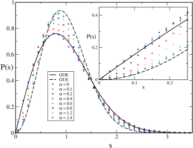
FIG. 1.: Level spacing distribution $P(s)$ for $\lambda=2$ and different fluxes $\alpha$. A transition between the Gaussian Orthogonal ($GOE$) and Gaussian Unitary ($GUE$) ensemble is observed as the flux is increased, even the asymptotic behavior of $P(s)$ is modified by the flux.

The number variance $\Sigma^{2}(L)=\langle L\rangle^{2}-\langle L^{2}\rangle=L-2\int_{0}^{L}ds(L-s)R_{2}(s,\alpha)$ ($R_{2}(s,\alpha)$ is the two level correlation function) measures the stiffness of the spectrum. Fluctuations are small in the metallic regime (Wigner-Dyson statistics) with $\Sigma^{2}(L)\sim\log(L)$ for $L\gg 1$. For localized eigenstates, the eigenvalues are uncorrelated (Poisson statistics) and $\Sigma^{2}(L)=L$. As mentioned earlier, the number variance is asymptotically proportional to $\chi L$ ($\chi<1$) at the MIT. In figure 3 we plot the number variance in the weak disorder regime ($\lambda=2$) for different flux values. As the flux is increased, a smooth transition is observed between critical $GOE$ [10, 9] and critical $GUE$ [8]. We remark the slope is not modified by the flux. This is in apparent disagreement with the results for a 2D Anderson model in the weak multifractality regime where the slope is two times smaller in the unitary case [20]. The reason for that is the way in which the flux is introduced due to the long range hopping. If the flux in (1) is introduced as usual in short range models the 2D Anderson model results are recovered. The asymptotically linear number variance (see fig 3) together with the level repulsion indicates that our model is described by critical statistics [6]. The strong disorder regime is explored by choosing a coupling constant ($\lambda=0.44$) such that the slope of the number variance $\chi\sim 0.29$ be similar to that at the 3D MIT. We observe (fig 4) that the flux only modifies the spectral correlations up to ($L\sim 1$) (see inset fig 4). Beyond this point the number variance is independent of the flux, thus suggesting that symmetry is washed out by disorder. We want to stress that the transition from weak to strong disorder is not sharp. As $\lambda$ decreases, the flux impact decreases smoothly. Curiously, until values of $\lambda$ very close to those at the 3D MIT, the effect, although small, is still sizable. Such behavior makes more difficult an accurate account of the flux at the 3D MIT. Finally let us mention that although not shown in the figures it was explicitly checked that the spectral correlators are not dependent on the size of the matrix as expected at a MIT.

FIG. 2.: P(s) for $\lambda=0.44$ and different fluxes. Only for $s\ll 1$ the system is sensitive to the flux. For $s\gg 1$ all curves become indistinguishable (inset).

After discussing the numerical results we propose an exact analytical relation for the two level correlation function of (1). We claim that such correlation function is equivalent to the dynamical density-density correlations of the CS model [11], ${{\hat{H}_{CS}}=-\sum_{j}\frac{\partial^{2}}{\partial x_{j}^{2}}+\frac{\beta(\beta-2)}{4}\sum_{i\neq j}\frac{1}{(x_{i}-x_{j})^{2}}+\frac{1}{4N^{2}}\sum_{j}x_{j}^{2}}$
at finite temperature where the position of the CS particles corresponds with the (unfolded) eigenenergies of (1), “time” $\sim\alpha^{2}$ and temperature $h$ is related to $\lambda$. Let us first argue how these density-density correlations are obtained [10, 21]. The density of probability of the CS ground state (zero temperature) for ($\beta=1,2,4$) is equivalent to the joint distribution of eigenvalue of the Gaussian random matrix models (GRMM). In the large $N$ limit, the two point spectral correlations of the GRMM are explicitly expressed through a spectral kernel. Such kernel in the language of the CS model corresponds with the amplitude of probability of having two free fermions in a ensemble of $N$ around two arbitrary positions. The idea is that, based on the Luttinger liquid nature of the CS model [24], the density-density correlations of the CS model at finite low temperature can be obtained by using the results of GRMM but replacing the spectral kernel above mentioned by its finite temperature analogue. In the grand canonical ensemble [8], $K(s=x-y,0)_{h}=\sum_{n}\frac{\psi_{n}(x)\psi^{\dagger}_{n}(y)}{1+z^{-1}e^{E_{n}/h}}$ where $\psi_{n}$ are the single particle wave functions for free fermions and $E_{n}=n/N$. In the large $N$ limit the wave functions are replaced by plane waves with energy given by $k^{2}$.

Dynamical density-density correlations [21] can be included in this formalism by expressing the time dependent density as $\rho(s,t\sim\alpha^{2})=e^{{\hat{H}_{CS}}t}\rho(s)e^{-{{\hat{H}}_{CS}}t}$. The crossover between orthogonal and unitary symmetry in the GRMM [20] corresponds in the language of the CS model with density-density correlations with initial conditions given by particles distributed according to the CS model for $\beta=1$ and then evolving for $t>0$ according to the CS model for $\beta=2$ (free fermions). The density-density correlations in this case [21] are also expressed through a spectral kernel as the one mentioned above but now involving the propagation of free fermions (hole and particle). Combining both effect, the dynamical (with the inital conditions above mentioned) density-density correlations of the CS model at finite temperature are given by (see [9, 21] for details),

$$\langle\rho(s,\alpha)\rho(0,0)\rangle_{h}-\langle\rho(s,\alpha)\rangle_{h}\langle\rho(0,0)\rangle_{h}=R_{2}(s,\alpha)_{h}=$$ (3)

$$K^{2}_{P}(s,0)_{h}-\left(\frac{d}{ds}K_{P}(s,\alpha)_{h}\right)\int_{s}^{\infty}{K_{H}}(s^{\prime},\alpha)_{h}ds^{\prime}$$ (4)

$$K_{P}(s,\alpha)_{h}=\int_{0}^{\infty}dkn_{P}(k){e^{\alpha^{2}u^{2}}\cos(\pi sk)}$$ (5)

$$K_{H}(s,\alpha)_{h}=\int_{0}^{\infty}dkn_{H}(k)e^{-\alpha^{2}k^{2}}\cos(\pi sk)$$ (6)

where $n_{H}(k)=1-n_{P}(k)=\frac{1}{1+ze^{k^{2}/h}}$ is the hole occupation number, $z=1/(e^{1/h}-1)$ is the fugacity, $\alpha$ is the magnetic flux (time), and $h$ is related to $\lambda$ by $2\pi h\sim 1/\lambda$ for $h\ll 1$ [16].

The $\alpha\rightarrow 0$ limit in (3) yields the density-density correlations of the CS model at finite temperature $h\ll 1$ [10, 9] which resembles the two point spectral correlations of a disordered system at the localization-delocalization transition. The limit $h\rightarrow 0$ corresponds with the exact analytical result for the crossover between orthogonal and unitary symmetry of a disordered system in the metallic regime [20] which is equivalent to the exact dynamical density-density correlations of the CS model [21].

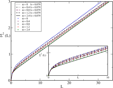
FIG. 3.: Number variance $\Sigma^{2}(L)$ for weak disorder $\lambda=2$ and different flux strengths. Lines are the analytical prediction (3) and symbols are the results obtained from the numerical diagonalization of (1) for $N=8000$.

The $s\gg 1,h\ll 1$ limit of (3) also agrees with the density-density correlations obtained in [24, 22] by using conformal field techniques.

Numerical calculations also support the validity of our conjecture. As observed in fig 3, the agreement between the analytical number variance based on (3) and the numerical result is excellent for the whole range of fluxes at $\lambda\sim 2$. We remark that no fitting is involved as the value of $h$ utilized corresponds with the analytical prediction $h=\frac{1}{2\pi\lambda}\sim 0.079$ [16]. In the strong disorder regime (see figure 4) the agreement is also remarkable but in this case no relation between $h$ in $\lambda$ is known so the parameter $h=0.267$ is the best fit to the numerical results. We want to point out that further work is needed to test whether the conjecture (3) is valid beyond the $h\ll 1$ limit.

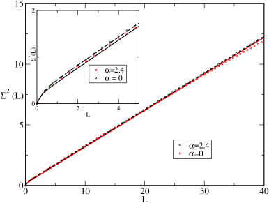
FIG. 4.: Number variance $\Sigma^{2}(L)$ for a disorder ($\lambda=0.44$) mimicking a true 3D Anderson transition. The lines represent the analytical prediction (3) ($h=0.267$) for no flux (segment) and maximum flux (solid). The symbols correspond to the numerical diagonalization of (1) for $N=8000$. The dependence on the flux observed for small $L\sim 1$ (see inset) is also reproduced by (3).

Finally we study the relation between classical and quantum properties of our model. For $\alpha=0,h\ll 1$, the two level spectral correlation function ($s\gg 1$) can be expressed through the spectral determinant of a diffusion operator [28] describing the classical dynamics of (1),

$$R_{2}(s) = -\frac{1}{2\pi^{2}}\frac{\partial^{2}G(s)}{\partial s^{2}}+2\cos(2\pi s)\,e^{2G(s)}$$ (7)

where, $e^{G(s)}=\frac{D(s)}{2\pi^{2}\,s^{2}}$,${D^{-1}(s)=\prod_{m\neq 0}\frac{{\epsilon_{m}}^{2}+s^{2}}{{\epsilon_{m}}^{2}}}$ is the spectral determinant and $\epsilon_{m}=m/h$ are the eigenvalues of the (anomalous) diffusion operator. As expected, the ($s\gg 1,\alpha=0$), limit of (3) coincides with (7). Unlike short range models, the type of classical diffusion associated with (1) is anomalous [23]. Such diffusion is described by a fractional Fokker-Planck equation [29]. For band decaying as $1/r^{\gamma}$, $1/2<\gamma<3/2$, the resulting classical dynamics is superdiffusive with $|r|\sim t^{1/(2\gamma-1)}$[16]. In the our case ($\gamma=1$) the associated fractional Fokker Planck equation is first order in space [30] and the eigenvalues of the diffusion operator (7) are thus linear in $m$ instead of quadratic as for normal diffusion. This link between anomalous classical motion and quantum correlations at the MIT may be utilized to find out conditions for the Anderson transition in quantum chaotic systems.

In conclusion, we have performed a numerical and analytical investigation in a 1D wire with long range disorder and a flux attached to it. In the weak disorder regime we have observed that despite the critical character of the model the effect of the flux is still important. By contrast, in the strong disorder limit, the spectral correlations are almost independent of the flux except for small eigenvalue separations. We have also conjectured, by exploiting an analogy with the CS model, an exact analytical relation for the spectral correlations at the MIT valid for arbitrary flux and disorder $h\ll 1$. We have suggested that, at least in 1D, the MIT, a quantum mechanic phenomenon, may be related with certain features of the classical dynamics (anomalous diffusion). We expect this relation to be relevant in quantum chaos problems.

Discussions with Gilles Montambaux and Patricio Leboeuf are gratefully acknowledged. This work was supported by the European Union network “Mathematical aspects of quantum chaos”.

REFERENCES

- [1] F. Wegner, Z. Phys. B 36, 209 (1980).
- [2] M. Janssen, Phys. Rep. 295, 1 (1998).
- [3] C. Castellani and L. Peliti, J. Phys. A: Math. Gen. 19, L429 (1986);H. Grussbach and M. Schreiber, Phys. Rev. B 45 (1993) 6650.
- [4] B.I. Shklovskii, B. Shapiro, B.R. Sears, P. Lambrianides and H.B. Shore, Phys. Rev. B 47, (1993) 11487.
- [5] B.L. Altshuler, I.K. Zharekeshev, S.A. Kotochigova and B.I. Shklovskii, JETP 67 (1988) 62.
- [6] V.E. Kravtsov and K.A. Muttalib, Phys. Rev. Lett. 79, 1913 (1997).
- [7] J.T. Chalker, I.V. Lerner, and R.A. Smith, Phys. Rev. Lett. 77, 554 (1996); J.T. Chalker, V.E. Kravtsov, and I.V. Lerner, Pis’ma Zh. Eksp. Teor. Fiz. 64, 355 (1996)
- [8] M. Moshe, H. Neuberger and B. Shapiro, Phys. Rev. Lett. 73, (1994) 1497; K.A. Muttalib, Y. Chen, M.E.H. Ismail and V.N. Nicopoulos, Phys. Rev. Lett. 71, (1993) 471.
- [9] A.M. Garcia-Garcia and J.J.M. Verbaarshot, Phys. Rev. E 67, 046104 (2003).
- [10] V.E. Kravtsov and A.M. Tsvelik, Phys. Rev. B 68, (2000) 9888.
- [11] B. Sutherland, J. Math. Phys. 12, 246 (1971);F. Calogero, J. Math. Phys. 10, 2191 (1969).
- [12] P.W. Anderson, Phys. Rev. 109, 1492 (1958).
- [13] G. Yeung and Y. Oono, Europhys. Lett. 4, 1061 (1987).
- [14] C.C. Yu, Phys.Rev.Lett. 63, (1989) 1160.
- [15] L.S. Levitov, Phys. Rev. Lett. 64, 547 (1990).
- [16] A.D. Mirlin, Y.V. Fyodorov, F.-M. Dittes, J. Quezada, and T.H. Seligman, Phys. Rev. E 54, 3221 (1996).
- [17] F. Evers and A.D. Mirlin, Phys.Rev.Lett. 84, (2000) 3690;E. Cuevas, M. Ortuno et.al. Phys. Rev. Lett. 88, (2002) 016401;I. Varga and D. Braum, Phys. Rev. B 61, (2000) R11859.
- [18] E. Hofstetter and M. Schreiber, Phys. Rev. Lett. 73, (1994) 3137.
- [19] M. Batsch, M. Schweitzer et.al Phys. Rev. Lett. 77, (1996) 1552.
- [20] A. Altland, S. Iida, K.B. Efetov, J. Phys. A 26, (1993) 3545; A. Pandey and M.L. Mehta, Commun.Math.Phys. 87, 449 (1983).
- [21] A. Pandey and P. Shukla, J.Phys. A, 24, (1991) 3907.
- [22] Z.N.C. Ha, Phys. Rev. Lett. 73, 1574 (1994).
- [23] R. Metzler and J. Klafter, Phys. Rep. 339, (2000) 1.
- [24] N. Kawakami and S. Yang, Phys. Rev. Lett. 67, (1991) 2493.
- [25] B.L. Altshuler and L.S. Levitov, Phys. Rep. 288, 487 (1997).
- [26] S. Nishigaki, Phys. Rev. E 59, (1999) 2853
- [27] V. I. Falko and K.B. Efetov, Phys. Rev. B 50, (1994) 11267.
- [28] A. V. Andreev and B. L. Altshuler, Phys. Rev. Lett. 75, (1995) 902.
- [29] G.M. Zaslavsky, Phys.Rep. 371, (2002) 461.
- [30] H.C. Fogedby, Phys. Rev. B 50, 1657 (1994).