Exact first-order density matrix for a $d$-dimensional harmonically confined Fermi gas at finite temperature

Abstract

We present an exact closed form expression for the finite temperature first-order density matrix of a harmonically trapped ideal Fermi gas in any dimension. This constitutes a much sought after generalization of the recent results in the literature, where exact expressions have been limited to quantities derived from the diagonal first-order density matrix. We compare our exact results with the Thomas-Fermi approximation (TFA) and demonstrate numerically that the TFA provides an excellent description of the first-order density matrix in the large-$N$ limit. As an interesting application, we derive a closed form expression for the finite temperature Hartree-Fock exchange energy of a two-dimensional parabolically confined quantum dot. We numerically test this exact result against the 2D TF exchange functional, and comment on the applicability of the local-density approximation (LDA) to the exchange energy of an inhomogeneous 2D Fermi gas.

I Introduction

The recent technical advances made by DeMarco and Jin jin in the area of trapped, ultra-cold Fermi gases, has led to the experimental realization of what is close to being an ideal, non-interacting, many-body system of harmonically confined fermions. Using current state-of-the art magneto-optical traps, it is also now possible to “tune” the dimensionality of the gas from three-dimensions (3D) to quasi-2D or quasi-1D. Such a model system is of great interest to physicists, as it provides an opportunity to study the role of dimensionality, and the quantum statistical properties of a many-body system, exactly. As a result, the last few years have seen a renewed interest in the theoretical description of harmonically trapped ideal Fermi gases at both zero vignolo1 ; gleisberg ; brack2 ; minguzzi1 ; minguzzi2 ; vignolo2 ; howard1 ; murthy and finite temperatures akdeniz ; brack1 . The primary focus of these studies has been on examining (analytically and numerically) the expressions for the local thermodynamic properties of the gas, e.g., the single-particle and kinetic energy densities. These quantities are, of course, of great importance in the density-functional theory (DFT) of inhomogeneous Fermi systems, whereby one can by-pass the numerically expensive one-particle Schrödinger equations.

However, the more fundamental quantity, from which the single-particle and kinetic energy densities are both derived, is the first-order density matrix $\rho_{1}({\bf r}_{1},{\bf r}_{2})$ parr . Unfortunately, to date, there are relatively few examples in which a closed analytical form for $\rho_{1}({\bf r}_{1},{\bf r}_{2})$ can be written. One of the earliest examples dates back more than 60 years to Husimi husimi , in which the zero temperature first-order density matrix of a 1D harmonic oscillator was derived. Other examples that we are aware of are the so-called Bardeen model bardeen , corresponding to a planar metal surface, and the work of Bhaduri and Sprung bhaduri_sprung dealing with a 3D oscillator with a smeared occupancy. More recently, Howard et. al howard have evaluated the zero temperature first-order density matrix of the $d$-dimensional harmonic oscillator for an arbitrary number of closed shells. Unfortunately, their form for $\rho_{1}({\bf r}_{1},{\bf r}_{2})$ is somewhat impractical in that it is given in terms of multidimensional integrals. While these integrals are numerically easy to evaluate, they are not very useful for further analytical analysis (e.g, examining the asymptotic behaviour of $\rho({\bf r})$ as $N\rightarrow\infty$ brack1 ; murthy ).

One of the central theoretical reasons for pursuing a closed form expression for $\rho_{1}({\bf r}_{1},{\bf r}_{2})$ is that its off-diagonal elements determine the exchange integrals of two-body operators, and hence, the nonlocal properties of the system. From an experimental point of view, a closed form expression for $\rho_{1}({\bf r}_{1},{\bf r}_{2})$ is desirable because, e.g., the momentum density $n({\bf p})$ (which is just the Fourier transform of the first-order density matrix), is experimentally accessible by measuring the line-shape in Compton scattering. Thus, in the case of a weakly-interacting harmonically confined Fermi gas, an exact knowledge of $\rho_{1}({\bf r}_{1},{\bf r}_{2})$ can serve as a benchmark from which the effects of interparticle interactions may be extracted.

The primary goal of this paper then, is to present an exact closed form analytical expression for the finite temperature first-order density matrix of a harmonically confined ideal Fermi in any dimension. We organize our paper as follows. In Sec. II, we briefly review some of the basic definitions given in brack2 ; brack1 , and then proceed to derive a closed form expression for the finite temperature first-order density matrix in arbitrary dimensions. Following this calculation, we compare our exact $\rho_{1}({\bf r}_{1},{\bf r}_{2})$ with the TFA in 2D and discuss the applicability of the LDA for describing the nonlocal properties of the 2D trapped gas. Then, in Sec. IV, we apply our results to construct a closed form expression for the finite temperature Hartree-Fock (HF) exchange energy density of a parabolically confined 2D quantum dot. We numerically investigate this exact exchange energy density and comment on its applicability in the context of the LDA. Finally, in Sec. V, we present a summary of our results and briefly highlight some interesting avenues for further investigation.

II First-order density matrix in $d$-dimensions

In keeping with our our earlier work brack1 ; brack2 , we begin by considering a system of noninteracting fermions at zero temperature described by the time-independent Schrödinger equation

$${\hat{H}}\phi_{i}({\bf r})=[\hat{T}+V({\bf r})]\phi_{i}({\bf r})=\varepsilon_{i}\phi_{i}({\bf r})~{},$$ (1)

where $V({\bf r})$ is a one-body potential to be specified later (all $\epsilon_{i}$’s are taken to be positive). The (spinless) first-order density matrix can be obtained by an inverse Laplace transform of the zero-temperature Bloch density matrix, $C_{0}({\bf r}_{1},{\bf r}_{2})$:

$$\rho_{1}({\bf r}_{1},{\bf r}_{2})=2\sum_{\varepsilon_{i}<E_{F}}\phi_{i}^{\star}({\bf r}_{2})\phi_{i}({\bf r}_{1})\Theta(E_{F})={\cal L}_{E_{F}}^{-1}\left[\frac{2}{\beta}C_{0}({\bf r}_{1},{\bf r}_{2};\beta)\right]~{},$$ (2)

where

$$C_{0}({\bf r}_{1},{\bf r}_{2};\beta)=\sum_{{\rm all~{}}i}\phi_{i}^{\star}({\bf r}_{2})\phi_{i}({\bf r}_{1})\exp(-\beta\varepsilon_{i})~{},$$ (3)

and $E_{F}$ is the Fermi energy; the factor of two accounts for spin. We have put in the unit step-function $\Theta(E_{F})$ in Eq. (2) so that the Laplace transform with respect to $E_{F}$ may formally be taken to be two-sided pol . Note that in quantum statistical mechanics, $\beta$ is usually identified with the inverse temperature, $\beta=1/k_{B}T$. However, in our present context, $\beta$ is to be interpreted as mathematical variable which in general is taken to be complex, and not the inverse temperature $1/k_{B}T$.

At finite temperature, the first-order density matrix is obtained from the Bloch density matrix by using the relation brack

$$\rho_{1}({\bf r}_{1},{\bf r}_{2};T)={\cal L}^{-1}_{\mu}\left[\frac{2}{\beta}C_{T}({\bf r}_{1},{\bf r}_{2};\beta)\right]~{},$$ (4)

where

$$C_{T}({\bf r}_{1},{\bf r}_{2};\beta)=C_{0}({\bf r}_{1},{\bf r}_{2};\beta)\frac{\pi\beta T}{\sin(\pi\beta T)}~{},$$ (5)

is the finite temperature Bloch density matrix, and $\mu$ is the chemical potential. In Eq. (4), the Laplace transform with respect to $\mu$ is two-sided, so that $\mu$ is allowed to go negative. Specializing now to the case of an isotropic harmonic oscillator in $d$ dimensions, viz.,

$$V({\bf r})=\frac{1}{2}m\omega^{2}r^{2},~{}~{}~{}~{}~{}~{}r=\sqrt{x_{1}^{2}+x_{2}^{2}+\cdot\cdot\cdot+x_{d}^{2}}~{},$$ (6)

we have for the zero-temperature Bloch density matrix wilson

$$C_{0}^{(d)}({\bf r}_{1},{\bf r}_{2};\beta)=C^{(d)}_{0}\left({\bf r}+\frac{{\bf s}}{2},{\bf r}-\frac{{\bf s}}{2};\beta\right)=\left(\frac{1}{2\pi}\right)^{d/2}\frac{1}{\sinh^{d/2}(\beta)}\exp\left\{-\left[r^{2}\tanh(\beta/2)+(s^{2}/4)\coth(\beta/2)\right]\right\}~{}.$$ (7)

In the above expression (and what follows), all lengths and energies have been scaled by $l_{osc}=\sqrt{\hbar/m\omega}$ and $\hbar\omega$, respectively, and we have introduced the center-of-mass and relative coordinates:

$${\bf r}=\frac{1}{2}({\bf r}_{1}+{\bf r}_{2}),~{}~{}~{}~{}~{}{\bf s}={\bf r}_{1}-{\bf r}_{2}~{}.$$ (8)

The finite temperature density matrix can, in principle, be obtained by performing the inverse Laplace transform given by Eq. (4) with Eq. (7). However, rather than following this direct approach (which is a very difficult task), we first consider the following identities

$$\exp\{-x\tanh(\beta/2)\} = \sum_{n=0}^{\infty}(-1)^{n}L_{n}(2x)e^{-x}\{e^{-n\beta}+e^{-(n+1)\beta}\}$$

$$\exp\{-y\coth(\beta/2)\} = \sum_{k=0}^{\infty}L_{k}(2y)e^{-y}\{e^{-k\beta}-e^{-(k+1)\beta}\}~{}.$$ (9)

Identifying $x=r^{2}$ and $y=s^{2}/4$, and using (9) in Eq. (7), the Bloch density matrix now reads

$$C_{0}^{(d)}(x,y;\beta) = \left(\frac{1}{2\pi}\right)^{d/2}\frac{1}{\sinh^{d/2}(\beta)}\sum_{k=0}^{\infty}\sum_{n=0}^{\infty}(-1)^{n}L_{n}(2x)L_{k}(2y)e^{-(x+y)}\{(e^{-n\beta}+e^{-(n+1)\beta})(e^{-k\beta}-e^{-(k+1)\beta})\}$$ (10)

$$= \left(\frac{1}{2\pi}\right)^{d/2}\frac{1}{\sinh^{d/2}(\beta)}\sum_{k=0}^{\infty}\sum_{n=0}^{\infty}(-1)^{n}L_{n}(2x)L_{k}(2y)e^{-(x+y)}\{e^{-(n+k)\beta}-e^{-(n+k+2)\beta}\}~{}.$$

Substituting Eq. (10) into Eq. (5) and performing the inverse Laplace transform, Eq. (4), leads to the finite temperature first-order density matrix $\rho_{1}({\bf r}_{1},{\bf r}_{2};T)$ in any dimension. For the sake of clarity, we will now proceed to give an explicit calculation for the simplest case of 2D, followed by a statement of the general result in arbitrary dimensions.

II.1 Two dimensions

We begin by noting the following important exact inverse Laplace transforms (all two-sided):

$${\cal L}^{-1}_{\eta}\left[\frac{e^{-n\beta}}{\sinh(\beta)}\right]=2\sum_{k=0}^{\infty}\delta(\eta-(2k+1)-n)~{}\Theta(\eta),$$ (11)

$${\cal L}^{-1}_{\mu}\left[\frac{\pi T}{\sin(\pi\beta T)}\right]=\frac{1}{\left[\exp(-\frac{\mu}{T})+1\right]}~{}.$$ (12)

Putting $d=2$ in Eq. (10) and using Eqs. (4), (5), the finite temperature first-order density matrix is given by

$$\rho_{1}^{(2)}(x,y;T)=\left(\frac{1}{\pi}\right)\sum_{k=0}^{\infty}\sum_{n=0}^{\infty}(-1)^{n}L_{n}(2x)L_{k}(2y)e^{-(x+y)}\\ \times{\cal L}_{\mu}^{-1}\left[\left(\frac{e^{-(n+k)\beta}-e^{-(n+k+2)\beta}}{\sinh(\beta)}\right)\frac{\pi T}{\sin(\pi\beta T)}\right]$$ (13)

Applying the convolution theorem for Laplace transforms and making use of Eqs. (11), (12), we immediately obtain

$$\rho_{1}^{(2)}(x,y;T) = \left(\frac{2}{\pi}\right)\sum_{k=0}^{\infty}\sum_{n=0}^{\infty}(-1)^{n}L_{n}(2x)L_{k}(2y)e^{-(x+y)}\times\sum_{l=0}^{\infty}\left\{\int_{-\infty}^{\infty}d\tau\delta(\tau-(2l+1)-(n+k))\frac{1}{\left[\exp(\frac{\tau-\mu}{T})+1\right]}\right.$$ (14)

$$- \left.\int_{-\infty}^{\infty}d\tau\delta(\tau-(2l+3)-(n+k))\frac{1}{\left[\exp(\frac{\tau-\mu}{T})+1\right]}\right\}$$

$$= \left(\frac{2}{\pi}\right)\sum_{k=0}^{\infty}\sum_{n=0}^{\infty}(-1)^{n}L_{n}(2x)L_{k}(2y)e^{-(x+y)}\times\sum_{l=0}^{\infty}\left\{\frac{1}{\left[\exp(\frac{2l+n+k+1-\mu}{T})+1\right]}-\frac{1}{\left[\exp(\frac{2l+n+k+3-\mu}{T})+1\right]}\right\}$$

$$= \left(\frac{2}{\pi}\right)\sum_{k=0}^{\infty}\sum_{n=0}^{\infty}(-1)^{n}L_{n}(2x)L_{k}(2y)e^{-(x+y)}\times\frac{1}{\left[\exp(\frac{\varepsilon_{n}+k-\mu}{T})+1\right]}$$

$$= \left(\frac{2}{\pi}\right)\sum_{k=0}^{\infty}\sum_{n=0}^{\infty}F^{(2)}_{n,k}(\mu)(-1)^{n}L_{n}(2x)L_{k}(2y)e^{-(x+y)}~{},$$

where the function $F^{(2)}_{n,k}(\mu)$ is defined as

$$F^{(2)}_{n,k}(\mu)\equiv\frac{1}{\left[\exp(\frac{\varepsilon_{n}+k-\mu}{T})+1\right]}~{},$$ (15)

and $\varepsilon_{n}=(n+1)$ is the noninteracting energy spectrum (in scaled units) of the 2D harmonic oscillator potential. Putting back our original variables, we finally arrive at the following simple expression

$$\rho_{1}^{(2)}({\bf r}_{1},{\bf r}_{2};T) = \left(\frac{2}{\pi}\right)\sum_{k=0}^{\infty}\sum_{n=0}^{\infty}F^{(2)}_{n,k}(\mu)(-1)^{n}L_{n}\left(\frac{|{\bf r}_{1}+{\bf r}_{2}|^{2}}{2}\right)L_{k}\left(\frac{|{\bf r}_{1}-{\bf r}_{2}|^{2}}{2}\right)$$ (16)

$$\times \exp\left(-\left|\frac{{\bf r}_{1}+{\bf r}_{2}}{2}\right|^{2}-\frac{|{\bf r}_{1}-{\bf r}_{2}|^{2}}{4}\right)~{}.$$

In terms of the center-of-mass and relative coordinates the density matrix is given by

$$\rho_{1}^{(2)}\left({\bf r}+\frac{{\bf s}}{2},{\bf r}-\frac{{\bf s}}{2};T\right) = \left(\frac{2}{\pi}\right)\sum_{k=0}^{\infty}\sum_{n=0}^{\infty}F^{(2)}_{n,k}(\mu)(-1)^{n}L_{n}\left(2r^{2}\right)L_{k}\left(\frac{s^{2}}{2}\right)\exp\left(-\left(r^{2}+\frac{s^{2}}{4}\right)\right)$$ (17)

Therefore, the density-matrix only depends on the modulus of ${\bf r}$ and ${\bf s}$, and there is a clean separation of the variables. Notice that Eq. (16) has only two sums owing to the cancellation of all but the $l=0$ term in the $l$-sum of Eq. (14). In addition, it is readily seen that by setting ${\bf r}={\bf r}_{1}={\bf r}_{2}$, we immediately obtain the finite temperature single-particle density

$$\rho_{1}^{(2)}({\bf r}_{1},{\bf r}_{1})\equiv\rho^{(2)}({\bf r};T)=\left(\frac{2}{\pi}\right)\sum_{n=0}^{\infty}F^{(2)}_{n}(\mu)(-1)^{n}L_{n}(2r^{2})e^{-r^{2}}~{},$$ (18)

with

$$F^{(2)}_{n}(\mu) \equiv \sum_{k=0}^{\infty}F^{(2)}_{n,k}(\mu)$$ (19)

$$= \sum_{k=0}^{\infty}\frac{1}{\left[\exp(\frac{\varepsilon_{n}+k-\mu}{T})+1\right]}~{}.$$

Equation (18) is of course identical to the result obtained in Ref. brack1 where only the diagonal part of the first-order density matrix was investigated. Furthermore, the exact 2D zero temperature density matrix can be obtained from Eq. (16) by taking the $T\rightarrow 0$ limit, and when filling $M+1$ shells, reduces to (with all dimensional constants recovered)

$$\rho^{(2)}_{1}({\bf r}_{1},{\bf r}_{2}) = \frac{2m\omega}{\pi\hbar}\sum_{n=0}^{M}(-1)^{n}L_{n}\left(\frac{m\omega}{2\hbar}|{\bf r}_{1}+{\bf r}_{2}|^{2}\right)L_{M-n}^{1}\left(\frac{m\omega}{2\hbar}|{\bf r}_{1}-{\bf r}_{2}|^{2}\right)\exp\left(-\frac{m\omega}{2\hbar}(r_{1}^{2}+r_{2}^{2})\right)$$ (20)

$$= \frac{2m\omega}{\pi\hbar}\sum_{n=0}^{M}(-1)^{n}L_{n}\left(\frac{2m\omega}{\hbar}r^{2}\right)L_{M-n}^{1}\left(\frac{m\omega}{2\hbar}s^{2}\right)\exp\left(-\frac{m\omega}{\hbar}\left(r^{2}+\frac{s^{2}}{4}\right)\right)$$

where $L_{M-n}^{1}(x)$ is an associated Laguerre polynomial gr [see also Eq. (34)] which has the property that $L_{M-n}^{1}(0)=M-n+1$. It is straightforward to show [with the aid of Eq. (35)] that Eq. (20) is indeed idempotent, viz.,

$$N=\int\int\rho_{1}^{(2)}({\bf r}_{1},{\bf r}_{2})\rho_{1}^{(2)}({\bf r}_{2},{\bf r}_{1})~{}d{\bf r}_{1}d{\bf r}_{2}~{}.$$ (21)

II.2 Arbitrary dimensions

The derivation of the first-order density matrix in arbitrary dimensions closely parallels that of the 2D case. The few extra steps required to obtain $\rho_{1}^{(d)}({\bf r}_{1},{\bf r}_{2};T)$ are clearly laid out in Ref. brack1 , and so here, we simply state the final result:

$$\rho_{1}^{(d)}({\bf r}_{1},{\bf r}_{2};T)=2\left(\frac{1}{\pi}\right)^{d/2}\sum_{k=0}^{\infty}\sum_{n=0}^{\infty}F_{n,k}^{(d)}(\mu)(-1)^{n}L_{n}\left(\frac{|{\bf r}_{1}+{\bf r}_{2}|^{2}}{2}\right)L_{k}\left(\frac{|{\bf r}_{1}-{\bf r}_{2}|^{2}}{2}\right)\exp\left(-\frac{1}{2}(r_{1}^{2}+r_{2}^{2})\right)~{},$$ (22)

where

$$F_{n,k}^{(d)}(\mu)\equiv\left(\frac{1}{\exp[(\varepsilon^{(d)}_{n}+k-\mu)/T]+1}+\sum_{m=1}^{\infty}\frac{g_{m}^{(d)}}{\exp[(\varepsilon^{(d)}_{n}+k+2m-\mu)/T]+1}\right)~{},$$ (23)

and $\varepsilon^{(d)}_{n}=n+d/2$. The expansion coefficients can be given in the compact form

$$g_{m}^{(d)} = \frac{1}{m!}\frac{\Gamma(d/2+m-1)}{\Gamma(d/2-1)}~{}.$$ (24)

In particular, we observe that $g_{m}^{(2)}=0$ for all $m$. We have verified the correctness of Eq. (22) at $T=0$ by checking that it is an exact solution of the partial differential equation (valid in any dimension)

$$\frac{1}{\xi\eta}\frac{\partial^{2}\rho_{1}(\xi,\eta)}{\partial\xi\partial\eta}=\frac{4m^{2}\omega^{2}}{\hbar^{2}}\rho_{1}(\xi,\eta)~{},$$ (25)

where following the notation of howard , we have defined $\xi=|{\bf r}_{1}+{\bf r}_{2}|/2$ and $\eta=|{\bf r}_{1}-{\bf r}_{2}|/2$ and

$$\rho^{(d)}_{1}(\xi,\eta)=2\left(\frac{1}{\pi}\right)^{d/2}\sum_{n=0}^{M}(-1)^{n}L_{n}(2\xi^{2})\left[L_{M-n}^{1}(2\eta^{2})+\sum_{m=1}^{(M-n)/2}g_{m}^{(d)}L_{M-n-2m}^{1}(2\eta^{2})\right]e^{-(\xi^{2}+\eta^{2})}~{}.$$

Equation (22) also provides us with a direct way to calculate the finite temperature kinetic energy density in any dimension, viz.,

$$\xi^{(d)}({\bf r};T)=-\frac{1}{2}\nabla_{s}^{2}\rho_{1}^{(d)}\left({\bf r}+\frac{{\bf s}}{2},{\bf r}-\frac{{\bf s}}{2};T\right)_{s=0}~{}.$$ (26)

This is an easier route compared with our previous evaluation of $\xi^{(d)}({\bf r};T)$, which required an additional inverse Laplace transform of the Bloch density matrix at finite temperature (see Eq. (33) of Ref. brack1 ). It should be noted that when making contact with experimental studies on fully spin-polarized trapped Fermi atoms, it is appropriate to focus on singly filled levels, which implies that the factor of two appearing in Eq. (22) should be dropped.

We also briefly mention that an analogous expression for $\rho_{1}^{(d)}({\bf r}_{1},{\bf r}_{2};T)$ for the harmonically trapped (spinless) Bose gas in any dimension can also be obtained by simply removing the factor of two in front of Eq. (22) and changing the $+1$ to $-1$ in the denominator of Eq. (23). While this resulting novel expression for the Bose gas is very different from what is found in the literature, it can be shown to be entirely equivalent to the more commonly used form brack1

$$\rho^{(d)}_{1}({\bf r}_{1},{\bf r}_{2};T) = \sum_{j=1}^{\infty}\frac{e^{j\mu/T}}{[\pi(1-e^{-2j/T})]^{d/2}}\times$$ (27)

$$\exp\left(-\frac{|{\bf r}_{1}+{\bf r}_{2}|^{2}}{4}\tanh(j/2T)-\frac{|{\bf r}_{1}-{\bf r}_{2}|^{2}}{4}\ \coth(j/2T)\right)~{}.$$

II.3 Second-order density matrix

In the present context of non-interacting fermions, the second-order density matrix, $\rho^{(d)}_{2}({\bf r}_{1}{\bf r}_{2},{\bf r}_{1}^{\prime}{\bf r}_{2}^{\prime})$ can immediately be obtained from our knowledge of $\rho_{1}^{(d)}({\bf r}_{1},{\bf r}_{2})$ (this is in the spirit of the HF approximation) parr . An important quantity derived from $\rho_{2}$ is its diagonal element, which corresponds to the pair density, and is given by:

$$\rho^{(d)}_{2}({\bf r}_{1}{\bf r}_{2},{\bf r}_{1}{\bf r}_{2})=\frac{1}{2}\left\{\rho^{(d)}({\bf r}_{1})\rho^{(d)}({\bf r}_{2})-\frac{1}{2}|\rho_{1}^{(d)}({\bf r}_{1},{\bf r}_{2})|^{2}\right\}~{}~{}~{}~{}~{}~{}{\rm[closed~{}shell]}~{}.$$ (28)

For example, in the HF approximation, the electron-electron potential energy is given by

$$V^{\rm HF}_{ee}=\int\int\frac{\rho^{(d)}_{2}({\bf r}_{1}{\bf r}_{2},{\bf r}_{1}{\bf r}_{2})}{|{\bf r}_{1}-{\bf r}_{2}|}d{\bf r}_{1}d{\bf r}_{2}~{},$$ (29)

so that the the first term in (28) is responsible for the classical Coulomb repulsion and the second term yields the quantum-statistical exchange energy.

III Comparison with the Thomas-Fermi approximation

In this section, we compare our exact expression for the first-order density matrix with that of the TFA. Since the largest deviations between the exact and TF results are known to be at low temperatures (and small particle numbers, especially in low-dimensional systems), we will restrict our comparisons to zero temperature, and simply state here that the temperature dependence of the exact $\rho_{1}({\bf r}_{1},{\bf r}_{2};T)$ is readily studied, should it be desirable. Again, for the sake of simplicity, we will focus explicitly on the 2D case, although the extension of the analysis to other dimensions is straightforward.

In the TFA, the 2D zero temperature Bloch density matrix is given by brack

$$C_{TF}({\bf r}_{1},{\bf r}_{2};\beta)=\left(\frac{1}{2\pi\beta}\right)e^{-\beta V[({\bf r}_{1}+{\bf r}_{2})/2]}e^{-|{\bf r}_{1}-{\bf r}_{2}|^{2}/2\beta}~{}.$$ (30)

Figure 1: Comparison of the exact zero temperature density matrix [Eq. (20) (solid curves)] with the TFA [Eq. (31) (dashed curves)] for various particle numbers. Panels (a)-(c) correspond to fixing the center-of-mass coordinate to ${\bf r}=0$, and panels (d)-(f) have ${\bf r}=3$. In all cases, $\rho_{1}$ is normalized to the central density in the trap, $\rho(0)$.

Figure 2: Comparison of the exact zero temperature density matrix [Eq. (20) (solid curves)] with the TFA [Eq. (31) (dashed curves)] for various particle numbers. Panels (a)-(c) correspond to fixing the relative coordinate to ${\bf s}=1$. In all cases, $\rho_{1}$ is normalized to the central density in the trap, $\rho(0)$. Note that at the classical turning point, the TF expression drops abruptly to zero.

The inverse Laplace transform given by Eq. (2) (with Eq. (30) for the Bloch density matrix) is readily performed, and we find for the 2D harmonically confined gas

$$\rho_{1}^{TF}({\bf r}_{1},{\bf r}_{2}) = \frac{1}{\pi}\sqrt{2\left(E_{F}-V\left(\frac{{\bf r}_{1}+{\bf r}_{2}}{2}\right)\right)}~{}J_{1}\left[\sqrt{2\left(E_{F}-V\left(\frac{{\bf r}_{1}+{\bf r}_{2}}{2}\right)\right)}|{\bf r}_{1}-{\bf r}_{2}|\right]\frac{1}{|{\bf r}_{1}-{\bf r}_{2}|}$$ (31)

$$= \frac{1}{\pi}\sqrt{2\left(E_{F}-V\left({\bf r}\right)\right)}J_{1}\left[\sqrt{2(E_{F}-V({\bf r}))}~{}s\right]\frac{1}{s}~{},$$

where $J_{1}(x)$ is a cylindrical Bessel function and it is understood that the right-hand side of Eq. (31) is multiplied by the unit step function $\Theta(E_{F}-V({\bf r}))$. Note that Eq. (31) is also an exact solution of Eq. (25). We immediately observe that for $E_{F}\gg V({\bf r})$ (i.e., far from the classical turning point, $r_{cl}$), Eq. (31) becomes effectively identical to the uniform gas result, viz., $V({\bf r})=0$. Thus, as $N\rightarrow\infty$, $r_{cl}\rightarrow\infty$, and the first-order density matrix is essentially unmodified by the trapping potential.

Now, it is far from obvious by simply looking at the functional forms of Eqs. (20) and (31) that the TF and exact expressions are even qualitatively similar. Indeed, it is well-known that for local properties, such as $\rho({\bf r})$, the TF and exact densities have very different qualitative behaviour, especially in low-dimensions and small particle numbers. In particular, the shell oscillations observed in the exact expressions are not reproduced by the (smooth) TF profiles brack2 . To address this issue, we show in Fig. 1 the exact zero temperature density matrix (solid curves) along with Eq. (31) (dashed curves) for various particle numbers. Let us first focus on the left panels [i.e., Fig. 1(a)-(c)] which correspond to fixing the center-of-mass coordinate to ${\bf r}=0$. We observe that for low-particle numbers, there is a sizable quantitative difference between the two expressions, but by $N\sim O(10^{3})$, the exact and TF expressions agree quite well. In particular, the spatial oscillations in the exact and TFA expressions are in almost quantitative agreement by Fig. 1(c). For the right panels (which have ${\bf r}=3$), we note the same trend, but now with the agreement between the two expressions noticeably improved (i.e., for the same number of particles). Similar behaviour is seen for other values of ${\bf r}$, clearly illustrating that even at moderate particle numbers, the LDA is a good description of $\rho_{1}({\bf r}_{1},{\bf r}_{2})$, as a function of the relative coordinate $s$.

In Fig. 2(a)-(c) we also compare the exact and TFA of $\rho_{1}$, but now with the relative coordinate fixed to $s=1$ and the center-of-mass coordinate allowed to vary. Note that fixing $s=0$ yields the zero temperature single-particle density, which has already been investigated in Ref. brack2 . While the overall spatial behaviour of the two expressions are in agreement, the TFA clearly does not reproduce the fine spatial oscillations in the exact expression, which are associated with shell-filling effects. The reason for this, of course, is due to the fact that the LDA fails to take into account the discrete nature of the energy level structure of the trap. We will come back to this point in the Sec. IV C below. Nevertheless, by $M=49$, the agreement between the exact and TF expression is quite good, except near the classical turning point, where the TF curves drop abruptly to zero.

While it is possible to show analytically the reduction of the zero temperature particle and kinetic energy densities to their TF forms, e.g., $\lim_{N\rightarrow\infty}\rho({\bf r})^{\rm exact}\rightarrow\rho_{\rm TF}({\bf r})$ brack1 ; murthy , we have not yet been able to analytically establish a similar result for $\rho({\bf r}_{1},{\bf r}_{2})$. The demonstration of this result is an interesting problem in its own right.

IV Exchange energy for a 2D quantum dot: Hartree-Fock approximation

As a simple application of our results, we now consider the evaluation of an exact closed form expression for the HF exchange energy suitable for the study of 2D parabolically confined quantum dots. Here, our motivation for focusing to strictly two dimensions is grounded in our previous findings for the local properties of the zero temperature trapped 2D Fermi gas. Specifically, in Ref. brack2 , we showed analytically the surprising result that the 2D TF functional for the kinetic-energy density (i.e., without gradient corrections), when integrated over all space, leads to the exact quantum mechanical kinetic energy. Moreover, we also demonstrated numerically that if the exact single-particle density is inserted into the 2D TF kinetic-energy functional, even the local shell oscillations are reproduced remarkably well footnote . Thus, the unique local and global properties of the trapped 2D system are reason enough for us to focus on two-dimensions. Nevertheless, we wish to re-emphasize that extending the following calculations to other dimensions requires nothing more than introducing the $d$-dimensional measure, which is given by

$$\int d^{d}r(...)=\frac{\pi^{d/2}}{\Gamma(d/2)}\int_{0}^{\infty}x^{d/2-1}dx(...)~{}.$$ (32)

For orientation, we will first consider the case for $T=0$ and then generalize the result to finite temperatures. After presenting our analytical expressions, we will close this section with some illustrative numerical results at zero temperature.

IV.1 Zero temperature

Before proceeding with the zero temperature calculation, let us first consider a particular class of integrals that invariably arise during our manipulations of $\rho_{1}({\bf r}_{1},{\bf r}_{2};T)$, irrespective of dimensionality and temperature, viz.,

$$I_{m,n}(\alpha,\beta,\gamma) = \int_{0}^{\infty}x^{\alpha}e^{-x}~{}L_{m}^{\beta}(x)L_{n}^{\gamma}(x)~{}dx,$$ (33)

where the associated Laguerre polynomials are defined by

$$L_{m}^{\beta}(x)=\sum_{k=0}^{m}\frac{(-1)^{k}}{k!}\frac{(m+\beta)!}{(m-k)!(\beta+k)!}x^{k}~{}.$$ (34)

Inserting Eq. (34) into (33) and integrating term by term, we are left with a double sum, which can be resummed in closed form to give note2

$$I_{m,n}(\alpha,\beta,\gamma)=\frac{\Gamma(1+\alpha)\Gamma(n+\gamma+1)\Gamma(\beta-\alpha+m)}{\Gamma(m+1)\Gamma(n+1)\Gamma(1+\gamma)\Gamma(\beta-\alpha)}~{}_{3}F_{2}[1+\alpha-\beta,-n,1+\alpha;1+\gamma,1+\alpha-\beta-m;1]~{},$$ (35)

where ${}_{3}F_{2}[a,b,c;d,e;z]$ is the generalized hypergeometric function gr . We are now ready to proceed with the calculation of HF exchange energy for the 2D quantum dot.

The HF exchange energy, in the terms of the variables ${\bf r}$ and ${\bf s}$, reads (hereby we set $e=1$):

$$E_{\rm ex} = -\frac{1}{4}\int\int\frac{|\rho_{1}\left({\bf r}+\frac{{\bf s}}{2},{\bf r}-\frac{{\bf s}}{2}\right)|^{2}}{s}d{\bf s}d{\bf r}$$ (36)

$$= -\frac{\pi}{2}\int\int_{0}^{\infty}\left|\rho_{1}\left({\bf r}+\frac{{\bf s}}{2},{\bf r}-\frac{{\bf s}}{2}\right)\right|^{2}dsd{\bf r}~{},$$

where, from Eq. (20),

$$\left|\rho_{1}\left({\bf r}+\frac{{\bf s}}{2},{\bf r}-\frac{{\bf s}}{2}\right)\right|^{2}=\frac{4}{\pi^{2}}\sum_{n=0}^{M}\sum_{k=0}^{M}(-1)^{n+k}L_{n}(2r^{2})L_{k}(2r^{2})e^{-2r^{2}}L_{M-n}^{1}(s^{2}/2)L_{M-k}^{1}(s^{2}/2)e^{-s^{2}/2}~{}.$$ (37)

Equation (36) can now be written as

$$E_{\rm ex}=-\frac{2}{\pi}\sum_{n=0}^{M}\sum_{k=0}^{M}(-1)^{n+k}\int L_{n}(2r^{2})L_{k}(2r^{2})e^{-2r^{2}}d{\bf r}\int_{0}^{\infty}L_{M-n}^{1}(s^{2}/2)L_{M-k}^{1}(s^{2}/2)e^{-s^{2}/2}ds~{}.$$ (38)

Going over to the variables $x=s^{2}/2$, $y=2r^{2}$ and making use of Eq. (35), viz.,

$$I_{m,n}(-1/2,1,1) = \int_{0}^{\infty}x^{-1/2}L_{m}^{1}(x)L_{n}^{1}(x)e^{-x}dx$$ (39)

$$= 2(m+1)(n+1)\frac{\Gamma(n+3/2)}{\Gamma(n+2)}~{}_{3}F_{2}\left[-\frac{1}{2},-m,\frac{1}{2};2,-n-\frac{1}{2};1\right]~{},$$

we obtain

$$E_{\rm ex} = -\frac{\sqrt{2}}{\pi}\sum_{n=0}^{M}\sum_{k=0}^{M}(-1)^{n+k}\int L_{n}(2r^{2})L_{k}(2r^{2})e^{-2r^{2}}d{\bf r}\int_{0}^{\infty}e^{-x}x^{-1/2}L_{M-n}^{1}(x)L_{M-k}^{1}(x)dx$$ (40)

$$= -{\sqrt{2}}\sum_{n=0}^{M}\sum_{k=0}^{M}(-1)^{n+k}(M-n+1)(M-k+1)\frac{\Gamma(M-n+3/2)}{\Gamma(M-n+2)}~{}_{3}F_{2}\left[-\frac{1}{2},n-M,\frac{1}{2};2,k-M-\frac{1}{2};1\right]$$

$$\times \int_{0}^{\infty}L_{n}(y)L_{k}(y)e^{-y}dy$$

$$= -\sqrt{2}\sum_{n=0}^{M}(M-n+1)^{2}\frac{\Gamma(M-n+3/2)}{\Gamma(M-n+2)}~{}_{3}F_{2}\left[-\frac{1}{2},n-M,\frac{1}{2};2,n-M-\frac{1}{2};1\right]~{}.$$

Equation (40) can be written in the more suggestive form

$$E_{\rm ex}=\int\varepsilon_{\rm x}({\bf r})d{\bf r}~{},$$ (41)

whereby we identify the exchange energy density as

$$\varepsilon_{\rm x}({\bf r}) = -2\frac{\sqrt{2}}{\pi}\sum_{n=0}^{M}\sum_{k=0}^{M}(-1)^{n+k}(M-n+1)(M-k+1)L_{n}(2r^{2})L_{k}(2r^{2})e^{-2r^{2}}$$ (42)

$$\times \frac{\Gamma(M-n+\frac{3}{2})}{\Gamma(M-n+2)}~{}_{3}F_{2}\left[-\frac{1}{2},n-M,\frac{1}{2};2,k-M-\frac{1}{2};1\right]~{}.$$

Note that the first line in Eq. (42) is $\propto[\rho({\bf r})]^{2}$. However, the terms in the second line of (42) (i.e., the hypergeometric and Gamma functions) prevent us from writing $\varepsilon_{\rm x}({\bf r})$ as a simple functional of $[\rho({\bf r})]^{2}$.

IV.2 Finite temperature

The finite temperature exchange is readily calculated from Eq. (36) by using Eq. (16) for the finite temperature first-order density matrix. The calculation is entirely analogous to the zero temperature result, with the central difference being that we now have to evaluate the integral [see Eq. (17)]

$$I_{m,n}(-1/2,0,0) = \int_{0}^{\infty}x^{-1/2}L_{m}(x)L_{n}(x)e^{-x}dx$$ (43)

$$= \frac{\Gamma(n+1/2)}{\Gamma(n+1)}~{}_{3}F_{2}\left[-m,\frac{1}{2},\frac{1}{2};\frac{1}{2}-n,1;1\right]~{}.$$

Our final result for the 2D finite temperature exchange energy is given by

$$E_{\rm ex}(T) = -\frac{\sqrt{2}}{\pi}\sum_{n=0}^{\infty}\sum_{n^{\prime}=0}^{\infty}\sum_{k=0}^{\infty}\sum_{k^{\prime}=0}^{\infty}(-1)^{n+n^{\prime}}F^{(2)}_{n,k}(\mu)F^{(2)}_{n^{\prime},k^{\prime}}(\mu)\frac{\Gamma(k^{\prime}+1/2)}{\Gamma(k^{\prime}+1)}~{}_{3}F_{2}\left[-k,\frac{1}{2},\frac{1}{2};\frac{1}{2}-k^{\prime},1;1\right]$$ (44)

$$\times \int L_{n}(2r^{2})L_{n^{\prime}}(2r^{2})e^{-2r^{2}}d{\bf r}$$

$$= -\frac{1}{\sqrt{2}}\sum_{n=0}^{\infty}\sum_{k=0}^{\infty}\sum_{k^{\prime}=0}^{\infty}F^{(2)}_{n,k}(\mu)F^{(2)}_{n,k^{\prime}}(\mu)\frac{\Gamma(k^{\prime}+1/2)}{\Gamma(k^{\prime}+1)}~{}_{3}F_{2}\left[-k,\frac{1}{2},\frac{1}{2};\frac{1}{2}-k^{\prime},1;1\right]~{}.$$

The finite temperature exchange energy density is similarly given by

$$\varepsilon_{\rm x}({\bf r};T) = -\frac{\sqrt{2}}{\pi}\sum_{n=0}^{\infty}\sum_{n^{\prime}=0}^{\infty}\sum_{k=0}^{\infty}\sum_{k^{\prime}=0}^{\infty}(-1)^{n+n^{\prime}}F^{(2)}_{n,k}(\mu)F^{(2)}_{n^{\prime},k^{\prime}}(\mu)L_{n}(2r^{2})L_{n^{\prime}}(2r^{2})e^{-2r^{2}}$$ (45)

$$\times \frac{\Gamma(k^{\prime}+1/2)}{\Gamma(k^{\prime}+1)}~{}_{3}F_{2}\left[-k,\frac{1}{2},\frac{1}{2};\frac{1}{2}-k^{\prime},1;1\right]~{}.$$

While Eq. (45) looks somewhat unwieldy, it turns out that the sums can be truncated relatively quickly, so that the temperature dependence can be numerically studied, should the need arise.

IV.3 Numerical results

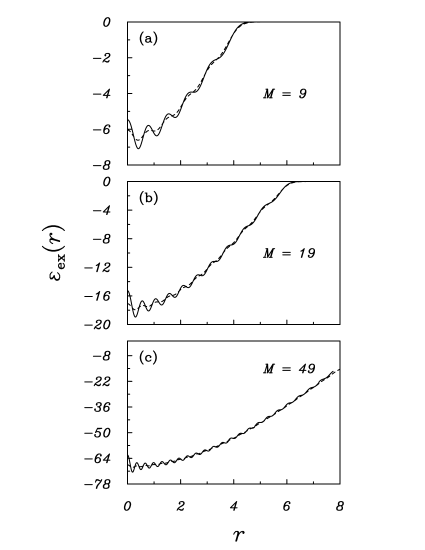
Figure 3: Comparison of the exact [Eq. (41), solid curves] and TF [Eq. (45), dashed curves] 2D exchange energy densities at zero-temperature, and various particle numbers. The TF exchange energy density has been generated by using the exact single-particle density as input [see Eq. (46)].

As mentioned above, the exact zero temperature kinetic energy density, $\tau({\bf r})$, for the trapped 2D Fermi gas agrees remarkably well with the corresponding TF expression, $T=\pi[\rho({\bf r})]^{2}/2$, when the exact $\rho({\bf r})$ is used as input (see Fig. 3 in Ref. brack2 ). It is then of interest to examine how well the 2D TF exchange energy density compares with the exact expression, Eq. (42), in both the small and large $N$-limit. Specifically, we will investigate the applicability of the well-known 2D Dirac exchange energy functional note3 ,

$$E^{\rm TF}_{\rm ex} = -\frac{4}{3}\sqrt{\frac{2}{\pi}}\int~{}[\rho({\bf r})]^{3/2}d{\bf r}$$ (46)

$$= \int\varepsilon_{\rm ex}^{\rm TF}({\bf r})~{}d{\bf r}~{},$$

for the inhomogeneous 2D gas when the exact density, as given by Eq. (20) with ${\bf r}_{1}={\bf r}_{2}$, is used as input. To this end, we present in Fig. 3 (a)-(c) the exact (solid curves) and TF (dashed curves) exchange energy densities for various particle numbers. It is clear from this figure that while both expressions have similar qualitative behaviour, the fine spatial oscillations (i.e., shell-filling effects) are not well reproduced by the TFA. This result is entirely expected considering our discussion in Sec. III in connection to Fig. 2(a)-(c). Specifically, in obtaining $\varepsilon_{\rm ex}^{\rm TF}(r)$, we have integrated over $s$, so that we are left only with the center-of-mass coordinate $r$. Therefore, even though the TFA for $\rho_{1}$ is quite good for the $s$ integration, its failings become apparent upon an examination of the exchange density as a function of $r$; the TFA for $\varepsilon_{\rm ex}(r)$ leads to a smooth, monotonically increasing profile because the resulting $r$-dependence is $\propto-[\rho^{\rm TF}({\bf r})]^{3/2}=-[(E_{F}-V({\bf r}))/\pi]^{3/2}$ [see Eq. (46) above]. However, in Fig. 3, $\varepsilon_{\rm ex}^{\rm TF}(r)$ has been obtained by using the exact single-particle density as input, which does have the shell effects encoded in its spatial dependence. Thus, although shell oscillations can be included in the TFA of $\varepsilon^{\rm TF}_{\rm ex}(r)$ (i.e., by using the exact density), it is important to note that for a given $r$, the weighting given to the Laguerre polynomials in $[\rho^{\rm exact}(r)]^{3/2}$ is not the same as the weight assigned to the Laguerre polynomials in Eq. (42). Consequently, the exchange energy densities do not agree as we vary the center-of-mass coordinate. We note in particular that the shell-effects in TFA are less pronounced than the exact result, and by $M=49$ and $r\gtrsim 3$, are essentially washed out [see Fig. 3(c)]. It is also worth recounting here, that by $M=19$ (see Fig. 3 in Ref. brack2 ), the deviations between the exact and TF 2D kinetic energy densities are essentially nonexistent; this is clearly not the case for the exchange energy density. The reasons behind the success of the TFA for the kinetic energy density are thoughoroughly discussed in Ref. murthy . Nevertheless, the numerics clearly indicate here that as $N\rightarrow\infty$, $\varepsilon_{\rm ex}^{\rm exact}(r)\rightarrow\varepsilon_{\rm ex}^{\rm TF}(r)$.

While the local behaviour of the exact and TF exchange energy densities are not well reproduced (as opposed to the comparatively superb agreement between the exact and TF kinetic energy densities), the exchange energy itself agrees remarkable well. To illustrate this, we show in Table I the exact and TF exchange energies for various numbers of filled shells. The largest relative percentage error, which occurs at $M+1=10$, is only $\Delta E/E\simeq 0.5\%$. Thus, when global quantities are considered, the LDA is an excellent approximation for the inhomogeneous 2D exchange energy, even for $N\sim O(10^{2})$.

$M+1~{}~{}$	$~{}~{}E_{\rm ex}^{\rm exact}~{}~{}$	$E_{\rm ex}^{\rm TF}~{}~{}$	$\Delta E/E$
10	-171.71	-170.81	0.5$\%$
20	-914.05	-912.43	0.2 $\%$
50	-8703.06	-8699.51	0.04 $\%$

Table 1: Comparison of the zero temperature exchange energy for the exact [Eq. (40)] and TF [Eq. (46)] expressions for various numbers of filled shells. The last column displays the relative percentage error in the two quantities.

V Summary and future work

The main result of this paper can be summarized by Eq. (22), which defines the exact, $d$-dimensional, finite temperature first-order density matrix of an ideal gas of harmonically confined fermions. This expression should prove to be of interest in the general area of the DFT of inhomogeneous Fermi systems at both zero and finite temperatures. In this paper, we have used it to illustrate that (in 2D) the LDA is an excellent approximation for the the off-diagonal first-order density matrix in the large-$N$ limit. We have also obtained a simple, closed form expression for the finite temperature exchange energy density for a 2D parabolically confined quantum dot. In the spirit of our previous work brack2 , we have utilized this exact expression to test the validity of the LDA for the exchange energy density. In contrast to our earlier findings brack2 , the 2D TF exchange energy functional does not reproduce the shell effects of the exact result very well. Nevertheless, when the TF exchange energy density is integrated over all space, we find that the resulting exchange energy is always within $\lesssim 0.5\%$ of the exact result.

We wish to point out that the utility of our results are not limited to the topics discussed in this paper. The simple, analytical expressions that we have provided will be very useful in the obtaining other closed form expressions of interest to both theorists working in formal DFT, and experimentalists studying e.g., ultra-cold trapped fermions. One example that comes to mind is the 2D weakly interacting trapped Fermi gas. In Ref. brack1 , the use of a contact psuedopotential (in 2D) led to the surprising discovery that there is no splitting between states with different angular momentum values $l$ in a given shell at $T=0$. This occurs in spite of the fact that the perturbation interaction does not preserve the $SU(2)$ symmetry of the system. Whether this result still holds true for a finite-range psuedopotential is an interesting question, which can be addressed using our analytical expression for $\rho_{1}({\bf r}_{1},{\bf r}_{2})$. In addition, the close connection between trapped Fermi gases and the theory of nuclear structure suggests that our findings will be relavent in the area of nuclear physics (e.g., in the Fermi gas model of the nucleus). Finally, our work here should also be useful in the physics of metal clusters, which represent an intermediate stage in the transition from small molecules to bulk solids or liquids.

References

• (1) B. DeMarco and D. S. Jin, Science 285, 1703 (1999); M. J. Holland, B. DeMarco, and D. S. Jin, Phys. Rev. A 61, 053610 (2000).
• (2) P. Vignolo, A. Minguzzi, and M. P. Tosi, Phys. Rev. Lett. 85, 2850 (2000).
• (3) F. Gleisberg, W. Wonneberger, U. SchlΓΆder, and C. Zimmermann, Phys. Rev. A 62, 063602 (2000).
• (4) M. Brack and B. P. van Zyl, Phys. Rev. Lett. 86, 1574 (2001).
• (5) A. Minguzzi, N. H. March and M. P. Tosi, Eur. Phys. J. D15, 315 (2001).
• (6) A. Minguzzi, N. H. March and M. P. Tosi, Phys. Lett. A 281, 192 (2001).
• (7) P. Vignolo and A. Minguzzi, J. Phys. B: At. Mol. Opt. Phys. 34, 4653 (2001).
• (8) I. A. Howard and N. H. March, J. Phys. A: Math. Gen. 34, L491 (2001).
• (9) M. V. N. Murth and M. Brack, J. Phys. A: Math. Gen. 36, 1111 (2003).
• (10) Z. Akdeniz, P. Vignolo, A. Minguzzi, and M. P. Tosi, Phys. Rev. A 66, 055601 (2002).
• (11) B. P. van Zyl, R. K. Bhaduri, A. Suzuki and M. Brack, Phys. Rev. A 67, 023609 (2003).
• (12) R. G. Parr and W. Yang, Density-Functional Theory of Atoms and Molecules, (Oxford University Press, New York, 1989).
• (13) K. Husimi, Proc. Phys. Math. Soc. Japan 22, 264 (1940).
• (14) J. Bardeen, Phys. Rev. 49, 653 (1936).
• (15) R. K. Bhaduri and D. W. L. Sprung, Nucl. Phys. A297, 365 (1978).
• (16) I. A. Howard, N. H. March and L. M. Nieto, J. Phys. A: Math. Gen. 35, 4985 (2002).
• (17) B. van der Pol and H. Bremmer, Operational Calculus, (Cambridge University Press, Cambridge, U.K.), Second Ed. (1955).
• (18) M. Brack and R. K. Bhaduri, Semiclassical Physics, Addison-Wesley, part of the Frontiers in Physics vol.Β 96 (1997).
• (19) E. H. Sondheimer and A. H. Wilson, Proc. R. Soc. London A 210, 173 (1951).
• (20) I. S. Gradshteyn and I. M. Ryzhik, Table of Integrals, Series, and Products (Academic Press, New York, 4th ed., 1994).
• (21) Similar agreement is also found for other dimensions. However, it is only the 2D system whose TF kinetic energy functional (with the exact density used as input) integrates to the exact quantum mechanical kinetic energy.
• (22) We have used the mathematical software package, MapleΒ©, to evaluate this quantity. We have also checked this result by hand.
• (23) This functional can easily be derived by using Eq.Β (31) in Eq.Β (36), and identifying $\rho({\bf r})=(E_{F}-V({\bf r}))/\pi$.