Conductance distribution in quasi-one-dimensional disordered quantum wires

Abstract

We develop a simple systematic method, valid for all strengths of disorder, to obtain analytically the full distribution of conductances $P(g)$ for a quasi one dimensional wire within the model of non-interacting fermions. The method has been used in [1, 2, 3] to predict sharp features in $P(g)$ near $g=1$ and the existence of non-analyticity in the conductance distribution in the insulating and crossover regimes, as well as to show how $P(g)$ changes from Gaussian to log-normal behavior as the disorder strength is increased. Here we provide many details of the method, including intermediate results that offer much insight into the nature of the solutions. In addition, we show within the same framework that while for metals $P(g)$ is a Gaussian around $\langle g\rangle\gg 1$, there exists a log-normal tail for $g\ll 1$, consistent with earlier field theory calculations. We also obtain several other results that compare very well with available exact results in the metallic and insulating regimes.

, and

1 Introduction

The absence of self-averaging in mesoscopic disordered conductors leads to important fluctuation effects in the electronic transport properties [4]. In the metallic regime, this gives rise to the universal conductance fluctuations [5]. In this regime, for a given strength of macroscopic disorder, the probability distribution $P(g)$ of the dimensionless conductance $g$ (in units of $e^{2}/h$), for all possible microscopic distributions of randomness, is a Gaussian with a universal variance i.e. its value does not depend on microscopic details of the sample but depends on the symmetry of the system only. With sufficiently large disorder however, the moments of the conductance fluctuations can become of the same order of magnitude as the average conductance, and therefore the average value becomes insufficient in describing the statistical properties of the conductor. In the extreme case of the deeply insulating regime, $P(g)$ becomes log-normal, which means that it has a very long tail so that its mean value is very different from the most probable value. Thus for all strengths of disorder beyond the metallic regime, one must consider the full distribution of conductances. In particular, a very broad distribution may change the qualitative nature of the Anderson transition, the metal to insulator transition at zero temperature even in the absence of electron-electron interactions [6]. The numerically obtained $P(g)$ at critical disorder for the three dimensional (3D) Anderson transition is indeed very broad and highly asymmetric [7]. The conductance at the integer quantum Hall transition is also expected to have a very broad, almost flat, distribution [8, 9].

There is no theoretical method currently available to obtain directly the full distribution of conductances for all strengths of disorder in arbitrary dimensions [10]. Moments of the distribution have been calculated in dimension $D=2+\epsilon$, $\epsilon\ll 1$ [11] within the supersymmetric non-linear sigma model framework [12] but the critical distribution obtained from the moments [13] in $D=2+\epsilon$ differ qualitatively from the numerically obtained $P(g)$ in 3D. In the present work we will consider the distribution of conductances for the simpler case of a quasi one dimensional (quasi 1D) wire, for which the width $W$ is smaller than the elastic mean free path $l$, and much smaller than its length $L$. Although such a system has no phase transition, it has well defined metallic and insulating regimes, and a smooth crossover between them. The distribution in the crossover regime, where the localization length is of the order of the system size, should give a reasonably good qualitative picture of the distribution near the critical regime in higher dimensions, where the localization length diverges and becomes of the order of the system size. Even for this simple quasi 1D geometry, only the first two moments of $P(g)$ have been obtained for all strengths of disorder [14], using the non-linear sigma model. Numerical [9, 15] as well as experimental [16] results show a broad asymmetric distribution qualitatively similar to 3D.

We will use a scattering approach in which the conductance is given in terms of the transmission eigenvalues $T_{i}$ of a finite conductor sandwiched between two ideal leads [17]. The finite width of the lead quantizes the perpendicular momenta into $N$ values, providing $N$ channels of scattering and therefore $N$ number of transmission levels. The dimensionless conductance $g$ is simply given by the total transmission probability

$$g=\sum_{i=1}^{N}T_{i}.$$ (1)

The statistics of these levels as a function of the length $L\gg l$ of the conductor is described by the Dorokhov-Mello-Pereyra-Kumar (DMPK) equation [18]. This equation has been shown [19] to be equivalent to the non-linear sigma model [12] obtained from the microscopic tight binding Anderson model, where electrons hop to neighboring sites that have random energies chosen from a uniform distribution. An advantage of using the DMPK equation is that its solution i.e. the joint probability distribution (jpd) of all the transmission eigenvalues is known [20] and since the conductance is simply related to these eigenvalues, it is possible to write down the full distribution of conductances. The major problem is that the jpd involves $N$ constrained integrals for the $N$ eigenvalues, and that we would be interested in the case of a large number of transmission eigenvalues.

We have developed a simple systematic method, valid for all strengths of disorder, to evaluate analytically the full distribution of conductance for a quasi 1d wire, starting from the solution of the DMPK equation. For simplicity, we restrict our calculation mostly to the unitary symmetry case where time reversal symmetry is broken, e.g. by the application of a magnetic field. The method is valid for other symmetry classes also, and we will discuss extension of the calculation to these cases as well. As a check of the essential framework, we will show analytically that the method reproduces the known exact results for the mean, variance as well as the distribution of the conductances in both the metallic and insulating limits. We will also compute the leading correction to the mean conductance in the metallic regime, which agrees very well with the exact value obtained in [14]. Since the leading order correction to the variance vanishes for the unitary symmetry class, we will evaluate it for the other two symmetry classes; again the results agree very well with the exact results. Also, it has already been shown in [2] that the mean and the variance as a function of disorder obtained within the method agrees qualitatively well with exact results for all strengths of disorder including the crossover regime.

Some of the novel features of the distribution obtained within our method have been reported earlier [1, 2, 3]. Here we discuss details which provide insights about the rare but allowed configurations of the transmission eigenvalues obtained from the method and allow us to study these features. In particular, we provide details that led to the prediction of a ‘one-sided’ log-normal distribution near the crossover regime in [1], the changes in the shape of the distribution across the crossover regime obtained in [2] as well as the non-analyticity in the distribution near $g=1$ predicted in [3]. We also show for the first time within DMPK that while for metals the distribution is a Gaussian around $\langle g\rangle\gg 1$, there exists a long non-Gaussian tail for $g\ll 1$, consistent with earlier field theoretic calculations [11].

The paper is organized as follows. In section 2 we review the DMPK equation and its general solution. In section 3 we introduce the basic strategy of our new approach which is used to evaluate $P(g)$ from the jpd of the $T_{i}$ for all strengths of disorder in terms of certain saddle point free energies. Our method is based on separating out an appropriate number of discrete eigenvalues and treating the rest as a continuum. For simplicity, we start with separating out only one eigenvalue in section 3. In section 4 we obtain explicit forms for the density of the continuum and various free energy terms. In this section we also discuss some of the special features in the density and their implications for the distribution. In section 5 we focus on the metallic regime and obtain several analytical results and compare them with known exact results. We also obtain the non-Gaussian tail of the distribution. In section 6 we obtain approximate analytic expressions for the distribution in the insulating and crossover regimes based on the separation of one eigenvalue. In section 7 we extend our formulation by separating out two eigenvalues, which have been used to obtain the non-analyticity in $P(g)$ near $g=1$ and also to evaluate the distribution across the crossover regime. In section 8 we briefly discuss the case of other symmetries, and obtain corrections to the mean and variance of $g$ and compare them with known exact results. We provide a summary and discuss conclusions in section 9.

2 Brief review of DMPK equation

For a quasi 1D wire with $N$ channels, as shown in Fig. 1, the probability distribution $p(\lambda)$ of the variables $\lambda_{i}=(1-T_{i})/T_{i}$, where $T_{i}$ are the transmission eigenvalues, satisfies the well known DMPK equation [18]

$$l\frac{\partial p}{\partial L}=\frac{2}{N+1}\frac{1}{J(\lambda)}\sum_{a}\frac{\partial}{\partial\lambda_{a}}\left[\lambda_{a}(1+\lambda_{a})J(\lambda)\frac{\partial p(\lambda)}{\partial\lambda_{a}}\right],$$ (2)

where $l$ is the mean free path, $J(\lambda)=\prod_{i<j}^{N}|\lambda_{i}-\lambda_{j}|^{\beta}$ and the parameter $\beta$ depends on the symmetry of the ensemble [24]: $\beta=1$ for orthogonal symmetry with time reversal invariance, $\beta=2$ for unitary symmetry where time reversal symmetry is broken by e.g. the application of a magnetic field, and $\beta=4$ for symplectic symmetry where e.g. spin-orbit scattering is present.

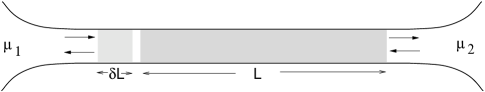
Figure 1: Quasi-one dimensional disordered wire attached to two electron reservoirs $\mu_{1},\mu_{2}$. The DMPK equation describe the evolution of the joint distribution of the transmission eigenvalues $T_{i}$ when system size L is increased e.g. by $\delta$L

The DMPK equation has been solved for all three values of $\beta$ [20, 21]. The general solution is complicated, but simplify in the metallic and insulating regimes. In these two regimes it can be written in the general form

$$p(\lambda)=\frac{1}{Z}\exp[-\beta H(\lambda)],$$ (3)

where $Z=\int\prod_{i}d\lambda_{i}\exp[-\beta H]$ is a normalizing factor independent of $\lambda_{i}$, and $H(\lambda)$ may be interpreted as the Hamiltonian function of $N$ classical charges at positions $\lambda_{i}$, interacting with a two-body repulsive interaction but confined by a one-body confinement potential, given as

$$H=\sum_{i<j}^{N}u(\lambda_{i},\lambda_{j})+\sum_{i}^{N}V(\lambda_{i}).$$ (4)

We will use the variables $\lambda_{i}=\sinh^{2}x_{i}$, in terms of which the solution in the metallic regime $1\ll L/l\ll N$ is given by

$$u(x_{i},x_{j})=-\frac{1}{2}\ln|\sinh^{2}x_{i}-\sinh^{2}x_{j}|-\frac{1}{2}\ln|x^{2}_{i}-x^{2}_{j}|,$$ (5)

$$V(x_{i})=\frac{\gamma l}{2L\beta}x^{2}_{i}-\frac{1}{2\beta}\ln|x_{i}\sinh 2x_{i}|..$$

Here $\gamma=\beta N+2-\beta$. In the insulating regime the solution is given by

$$u_{ins}(x_{i},x_{j})=-\frac{1}{2}\ln|\sinh^{2}x_{i}-\sinh^{2}x_{j}|-\frac{1}{\beta}\ln|x^{2}_{i}-x^{2}_{j}|,$$ (6)

$$V(x_{i})=\frac{\gamma l}{2L\beta}x^{2}_{i}-\frac{1}{2\beta}\ln|x_{i}\sinh 2x_{i}|-\frac{1}{2\beta}\ln x_{i}.$$

The parameters $N$, $L$ and $l$ appear in the above expressions in the combinations $L/l$ and $\Gamma=Nl/L$. We will consider the limit where both $N$ and $L$ approach infinity, keeping $\Gamma$ fixed. The limit $\Gamma\gg 1$ will correspond to the metallic regime while $\Gamma\ll 1$ will correspond to the localized regime. Note that for $\beta=2$, the solution in the insulating regime differs from the solution in the metallic regime only by a logarithmic term in the one-body potential.

In terms of the variables $\lambda_{i}$ or $x_{i}$, the dimensionless conductance is given by

$$g=\sum_{i}^{N}\frac{1}{1+\lambda_{i}}=\sum_{i}^{N}\frac{1}{\cosh^{2}x_{i}}.$$ (7)

In the insulating regime, $\langle g\rangle\ll 1$ and $x_{i}\gg 1$. In this limit both $\ln x_{i}$ and $\ln|x^{2}_{i}-x^{2}_{j}|$ terms in Eq. (6) are negligible compared to the other terms. Since these are the only terms that differ from Eq. (5), we can assume that the metallic expression (5) is valid for all regimes.

In the metallic regime $\langle g\rangle\gg 1$, the $\lambda_{i}$ are very close to each other so that a continuum description can be used with a density of $\lambda$ points finite between zero and an upper cutoff given by the normalization condition. Strictly speaking, Eq. (3) is valid only for $x^{2}>2/\beta\Gamma$ [21], but this approximation works well in the metallic regime. Within a global maximum entropy ansatz, such a continuum approximation was used [22] to show the relevance of a Wigner-Dyson like random matrix ensemble [25] for the transmission levels. The density of levels obtained from the DMPK solution within such a continuum approximation yields the correct value of the mean and the variance in the metallic regime [20], known from diagrammatic perturbation theory [5]. In the deeply insulating regime on the other hand, all $\lambda_{i}$ are exponentially large and separated exponentially from each other, and conductance is dominated by the smallest eigenvalue. This approximation yields the log-normal distribution of the conductance in the deeply insulating regime [23, 20]. It is clear however that none of the above descriptions can be used in the crossover regime, where the smallest eigenvalue is neither zero, nor exponentially large. Our approach combines the essential features of the two descriptions and provides a simple and systematic procedure to study the conductance distribution $P(g)$ at all strengths of disorder.

3 Generalized saddle point approximation for $P(g)$

Given the joint probability distribution $p(\lambda)$ and the definition of $g$ Eq. (7), the distribution of conductance can be written as

$$P(g)=\frac{1}{Z}\int_{-\infty}^{\infty}\frac{d\tau}{2\pi}\int_{0}^{\infty}\prod_{i=1}^{N}d\lambda_{i}\exp\left[i\tau\left(g-\sum_{i}^{N}\frac{1}{1+\lambda_{i}}\right)\right]p(\lambda).$$ (8)

For later use, we define a “Free energy”

$$F(\lambda;\tau)=\sum_{i}^{N}\frac{i\tau}{1+\lambda_{i}}+\beta H$$ (9)

such that the distribution of $g$ can be written as

$$P(g)=\frac{1}{Z}\int_{-\infty}^{\infty}\frac{d\tau}{2\pi}e^{i\tau g}\int_{0}^{\infty}\prod_{i=1}^{N}d\lambda_{i}\exp\left[-F(\lambda;\tau)\right].$$ (10)

This defines a statistical mechanical problem of $N$ classical charges in one dimension, at an inverse temperature $\beta$ and described by the free energy $F$, which includes a source term proportional to $\tau$. The basic idea of our method is to first separate out an appropriate number of the lowest eigenvalues, and treat the rest as a continuum by introducing a density for those eigenvalues. In [1] a single eigenvalue was separated out, which was sufficient to obtain the qualitative nature of $P(g)$ in the metallic regime, in the crossover region on the insulating side as well as deep in the insulating regime. In [2, 3], the importance of separating at least two eigenvalues in order to study the crossover region quantitatively was emphasized. However here we will consider in detail the case of separating out one eigenvalue in the metallic regime since it allows us to obtain many of our results analytically, which provides much insight into the nature of the solutions, and two eigenvalues in the crossover and insulating regimes where it becomes essential. The ‘density’ of the continuum, including the source term, is obtained following Dyson [24] by minimizing the free energy functional, which then yields a saddle point free energy. The qualitative nature of the density gives important information about the problem and will not only provide guidelines for appropriate approximations, but will also suggest novel possibilities in the distribution. We will see that at least for $\beta=2$, the $\tau$ dependence of $F(\lambda;\tau)$ is only quadratic, so the integral over $\tau$ in (10) can be done exactly. The evaluation of $P(g)$ is then reduced to two integrals in the metallic regime and three integrals in the crossover and insulating regimes, over all possible positions of the separated discrete levels, as well as over the beginning of the continuum. These integrals can then be done approximately analytically in some limiting cases to obtain qualitative results, or numerically to obtain quantitative results for comparison with direct numerical simulations. While we will mainly restrict our considerations to the case $\beta=2$ only, we would point out the results for other values of $\beta$ whenever they can be obtained without too much difficulty.

In the following, we will discuss the steps in more detail.

3.1 Separation of the lowest eigenvalue

We start by separating out only the lowest eigenvalue from the rest. This will be sufficient to study the metallic regime. In Sec. 7, we will show how to add a second discrete level, and write down the rules to extend the one-discrete level formulae to the two-discrete level case. This will keep the discussion of the basic framework simpler.

In the variable $x_{i}$, we get

$$H=H_{1}+\sum_{1<i<j}u(x_{i},x_{j})+\sum_{i>1}V(x_{i}),$$ (11)

where

$$H_{1}=\sum_{i>1}u(x_{i},x_{1})+V(x_{1}).$$ (12)

The idea is to treat the rest as a continuum, beginning at $x_{2}>x_{1}$.

3.2 Continuum approximation for the remaining eigenvalues

Before going to a continuum description, we note that $u(x_{i},x_{j})$ can be written as

$$u(x_{i},x_{j})=u^{\prime}(x_{i}-x_{j})+u^{\prime}(x_{i}+x_{j}),$$ (13)

$$u^{\prime}(x)=-\frac{1}{2}\ln(2x\sinh x).$$

The continuum description will then include the $x_{i}=x_{j}$ terms in $u^{\prime}(x_{i}+x_{j})$ which are not included in the discrete part. In order to get rid of these terms we rewrite the sum Eq. (11) as

$$H = H_{1}$$ (14)

$$+ \sum_{i>1}V(x_{i})+\frac{1}{2}\left[\sum_{1<i\neq j}u^{\prime}(x_{i}-x_{j})+\sum_{i,j>1}u^{\prime}(x_{i}+x_{j})-\sum_{i>1}u^{\prime}(2x_{i})\right].$$

The $x_{i}=x_{j}$ terms in $u^{\prime}(x_{i}-x_{j})$ are infinite, and will not make a difference in the continuum limit. Using in addition the expressions for $V(x_{i})$ and $u^{\prime}_{2}(2x_{i})$, we obtain

$$H=H_{1}+\frac{1}{2}\sum_{i,j>1}u(x_{i},x_{j})+\sum_{i>1}\left[V_{\Gamma}(x_{i})+2\alpha\ln(x_{i}\sinh 2x_{i})\right],$$ (15)

where

$$V_{\Gamma}(x_{i})=\frac{\Gamma}{2}x^{2}_{i}\hskip 19.91684pt\alpha=\frac{1}{8}\left(1-\frac{2}{\beta}\right)$$ (16)

Thus for $\beta=2$, the term proportional to $\alpha$ drops out.

The continuum approximation can now be made, giving for $\beta=2:$

$$H(x_{1},x_{2};\sigma(x)) = V(x_{1})+\int_{x_{2}}^{b}dx\sigma(x)u(x,x_{1})+\int_{x_{2}}^{b}dx\sigma(x)V_{\Gamma}(x)$$ (17)

$$+ \frac{1}{2}\int_{x_{2}}^{b}dx\int_{x_{2}}^{b}dx^{\prime}\sigma(x)u(x,x^{\prime})\sigma(x^{\prime})$$

where

$$V(x_{1})=\frac{\Gamma}{2}x^{2}_{1}-\frac{1}{2\beta}\ln(x_{1}\sinh 2x_{1})$$ (18)

and the ‘density’ $\sigma(x)$ has to be obtained in a consistent way, subject to the condition that it is positive everywhere. The upper limit $b$ in principle should take care of the normalization condition

$$\int_{x_{2}}^{b}\sigma(x)dx=N-1.$$ (19)

However, we will be interested in the $N\rightarrow\infty$ limit, and since the contributions to the conductance from large eigenvalues are negligible, we will not worry about enforcing the normalization condition and replace the upper limit by $\infty$. The Free energy can now be written in the continuum approximation as

$$F(x_{1},x_{2};\sigma(x))=\beta H(x_{1},x_{2};\sigma(x))+\frac{i\tau}{\cosh^{2}x_{1}}+i\tau\int_{x_{2}}^{\infty}\frac{\sigma(x)}{\cosh^{2}x}dx$$ (20)

and $P(g)$ is given by a functional integral on the generalized density $\sigma(x)$:

$$P(g)=\frac{1}{Z}\int_{-\infty}^{\infty}\frac{d\tau}{2\pi}e^{i\tau g}\int_{0}^{\infty}dx_{1}\int_{x_{1}}^{\infty}dx_{2}\int D[\sigma(x)]\exp[-F(x_{1},x_{2};\sigma(x))].$$ (21)

3.3 Integral equation for the saddle point density

We now minimize the free energy functional by taking a functional derivative with respect to $\sigma(x)$ keeping $x_{1}$ and $x_{2}$ fixed:

$$\frac{\delta F(x_{1},x_{2};\sigma(x))}{\delta\sigma(x)}=0.$$ (22)

This gives an integral equation for the saddle point density. We will see later that because the saddle point density goes to zero close to the origin, we will need to consider fluctuation corrections to the saddle point function.

Following Dyson (generalized for the non-logarithmic interaction case in [20]), we have the saddle point equation for $\sigma(x)$:

$$-\int_{x_{2}}^{\infty}dy\sigma(y)u(x,y)+4\alpha\left[\ln\sigma(x)+\delta u(x,y)+\frac{l}{L}x^{2}\right]=V_{tot}(x)+{\rm const,}$$ (23)

where $\delta u(x,y)=u(x,y)+\ln|x-y|$. Here $V_{tot}$ now includes

$$V_{tot}(x)=V_{\Gamma}(x)+u(x,x_{1})+\frac{i\tau}{\cosh^{2}x}.$$ (24)

Again the term proportional to $\alpha$ drops out for $\beta=2$.

3.4 The shift approximation

We define

$$u_{1}=\ln|\sinh^{2}x-\sinh^{2}y|;\;\;\;u_{2}=\ln|x^{2}-y^{2}|,$$ (25)

so that $u(x,y)=-\frac{1}{2}(u_{1}+u_{2})$. Then Eq. (23) for $\beta=2$ becomes

$$\int_{x_{2}}^{\infty}dy\sigma(y)[u_{1}(x,y)+u_{2}(x,y)]=2V_{tot}(x)+{\rm const};\;\;\;\;x>x_{2}.$$ (26)

In the limit $x_{2}\rightarrow 0$, the density can be extended symmetrically to negative values which makes it possible to invert the kernel and obtain $\sigma(x)$. Here the finite lower limit poses difficulty. A shift in the variables $x$ and $y$ to make the lower limit zero does not help, because the kernels are not translationally invariant. However in the variable $\lambda$, the kernel $u_{1}(\lambda-\lambda^{\prime})=\ln|\lambda-\lambda^{\prime}|$ is translationally invariant while $u_{2}(\lambda,\lambda^{\prime})=\ln|{\rm arsinh}\sqrt{\lambda}-{\rm arsinh}\sqrt{\lambda^{\prime}}|$ remains invariant for a metal ($\lambda\ll 1$), and is negligible in the insulating regime ($\lambda\gg 1$) compared to $u_{1}$. This suggests the following shift approximation to leading order, to which systematic corrections can be made:

(i) Write the integral equation in variable $\lambda$

$$\int_{\lambda_{2}}^{\infty}d\lambda^{\prime}[u_{1}(\lambda-\lambda^{\prime})+u_{2}(\lambda,\lambda^{\prime})]\rho(\lambda^{\prime})=2V_{tot}(\lambda).$$ (27)

where $\rho(\lambda^{\prime})d\lambda^{\prime}=\sigma(x)dx$. Now shift to $\eta=\lambda-\lambda_{2},$ and $\eta^{\prime}=\lambda^{\prime}-\lambda_{2}$ to make the lower limit zero:

$$\int_{0}^{\infty}d\eta^{\prime}[u_{1}(\eta-\eta^{\prime})+u_{2}(\eta+\lambda_{2},\eta^{\prime}+\lambda_{2})]\rho(\eta^{\prime}+\lambda_{2})=2V_{tot}(\eta+\lambda_{2}).$$ (28)

(ii) Write $u_{2}(\eta+\lambda_{2},\eta^{\prime}+\lambda_{2})=u_{2}(\eta,\eta^{\prime})+\Delta u_{2}$ where

$$\Delta u_{2}(\eta,\eta^{\prime};\lambda_{2})=\ln\frac{{\rm arsinh}^{2}\sqrt{\eta+\lambda_{2}}-{\rm arsinh}^{2}\sqrt{\eta^{\prime}+\lambda_{2}}}{{\rm arsinh}^{2}\sqrt{\eta}-{\rm arsinh}^{2}\sqrt{\eta^{\prime}}}.$$ (29)

For both $\eta\gg\lambda_{2}$ and $\eta\ll\lambda_{2}$, $\Delta u_{2}$ is negligible. In the metallic regime, the leading term of $\Delta u_{2}$ is a small correction linear in $\lambda_{2}$. So, for $\lambda_{2}\ll 1$ it is given by

$$\Delta u_{2}(\eta,\eta^{\prime};\lambda_{2})=\frac{\lambda_{2}}{{\rm arsinh}^{2}\sqrt{\eta}-{\rm arsinh}^{2}\sqrt{\eta^{\prime}}}\left[\frac{{\rm arsinh}\sqrt{\eta}}{\sqrt{\eta(1+\eta)}}-\frac{{\rm arsinh}\sqrt{\eta^{\prime}}}{\sqrt{\eta^{\prime}(1+\eta^{\prime})}}\right].$$ (30)

In the opposite limit i.e. in the insulating regime ($\lambda_{2}\gg 1$), the entire term $u_{2}$ is negligible compared to $u_{1}$. Therefore we will keep the leading term of $\Delta u_{2}$ as a small correction to the free energy in the metallic regime only. Its contribution to the saddle point density itself would be negligible. In this spirit, we make the approximation:

$$\int_{0}^{\infty}d\eta^{\prime}\Delta u_{2}(\eta,\eta^{\prime};\lambda_{2})\rho(\eta^{\prime}+\lambda_{2})\approx\int_{0}^{\infty}d\eta^{\prime}\Delta u_{2}(\eta,\eta^{\prime};\lambda_{2})\rho_{sp}(\eta^{\prime}+\lambda_{2}),$$ (31)

where the saddle point density $\rho_{sp}$ is the density obtained from the saddle point integral equation in the absence of the $\Delta u_{2}$ term. Then the integral equation (27) can be rewritten with the $\Delta u_{2}$ term taken to the right hand side to add to the $V_{tot}$, giving

$$\int_{0}^{\infty}d\eta^{\prime}[u_{1}(\eta-\eta^{\prime})+u_{2}(\eta,\eta^{\prime})]\rho_{sp}(\eta^{\prime}+\lambda_{2})=2V_{eff}(\eta;\lambda_{2}),$$ (32)

where the effective potential $V_{eff}$ is defined as $V_{eff}(\eta;\lambda_{2})=V_{tot}(\eta+\lambda_{2})-V_{2}(\eta;\lambda_{2})$, with $V_{tot}(x)$ defined in (24) and

$$V_{2}(\eta;\lambda_{2})=\frac{1}{2}\int_{0}^{\infty}d\eta^{\prime}\Delta u_{2}(\eta,\eta^{\prime};\lambda_{2})\rho_{sp}(\eta^{\prime}+\lambda_{2}).$$ (33)

In the crossover and insulating regimes, we will take $V_{2}=0$, since $\Delta u_{2}$ is negligible in these regimes.

(iii) Now change the variables in the saddle point equation (32):

$$\sinh^{2}t=\eta=\lambda-\lambda_{2},\;\;\;\sinh^{2}s=\eta^{\prime}=\lambda^{\prime}-\lambda_{2}$$ (34)

$$\int_{0}^{\infty}ds\left[\ln|\sinh^{2}t-\sinh^{2}s|+\ln|t^{2}-s^{2}|\right]\sigma(s)=2V_{eff}(\eta(t)+\lambda_{2}).$$ (35)

where we have defined

$$\sigma(s)=\rho_{sp}(\eta^{\prime}+\lambda_{2})\frac{d\eta^{\prime}}{ds}=2\sinh s\cosh s\;\rho_{sp}(\eta^{\prime}+\lambda_{2}).$$ (36)

Defining $\sigma(-s)=\sigma(s)$ we extend the density symmetrically to negative $s$ and using the relation: $\sinh^{2}t-\sinh^{2}s=\sinh(t-s)\sinh(t+s)$, the integral (35) can also be extended to $-\infty$, giving

$$\int_{-\infty}^{\infty}ds[\ln|\sinh(t-s)|+\ln|t-s|]\sigma(s)=2V_{eff}(\eta(t)+\lambda_{2}).$$ (37)

Since $\eta(-s)=\eta(s)$, this is true for all $s$.

(iv) Taking a derivative on both sides of the integral equation, we get

$$\int_{-\infty}^{\infty}dsK(t-s)\sigma(s)=2\frac{d}{dt}V_{eff}(\eta(t)+\lambda_{2})$$ (38)

where the kernel

$$K(t-s)=\coth(t-s)+\frac{1}{t-s}.$$ (39)

This kernel $K(t)$ can be inverted to give the saddle point density

$$\sigma(t)=2\int_{-\infty}^{\infty}dsK^{-1}(t-s)\frac{d}{ds}V_{eff}(\eta(s)+\lambda_{2}).$$ (40)

Using Fourier transform, we invert the kernels $K_{1}(t)=1/t$ and $K_{2}(t)=\coth t$ to obtain $K_{1}(q)=i\pi sign(q)$ and $K_{2}(q)=i\pi\coth(\pi q/2)$. Then using $\sigma(q)=[K_{1}(q)+K_{2}(q)]^{-1}\;2V^{\prime}_{eff}(q)$ we write

$$K^{-1}(t)=\int_{-\infty}^{\infty}\frac{dq}{2\pi}\frac{e^{-iqt}}{K_{1}(q)+K_{2}(q)}=-\frac{1}{\pi^{2}}\int_{0}^{\infty}dq\sin(qt)\frac{1}{2}(1-e^{-\pi q}).$$ (41)

Finally, introducing Eq. (41) into (40), the saddle point density is given by

$$\sigma(t)=\frac{2}{\pi^{2}}\int_{0}^{\infty}dq\cos(qt)(1-e^{-\pi q})\int_{0}^{\infty}ds\sin(qs)\frac{d}{ds}V_{eff}(\eta(s)+\lambda_{2}),$$ (42)

using the fact that $V_{eff}$ is even in $s$. Note that for $\beta\neq 2$, there would be additional terms in $V_{eff}$ proportional to the parameter $\alpha$.

3.5 Contributions to the Free energy

From the saddle point density, we obtain the saddle point Free energy by using the right hand side of the integral equation (23) to eliminate one of the two integrals of the last term in Eq. (17). Substituting this result into Eq. (20) and changing to the $\lambda$ variable (since shift has to be made in the $\lambda$ variable), we write the Free energy as

$$F_{sp}(\lambda_{1},\lambda_{2})=\frac{\beta}{2}\int_{\lambda_{2}}^{\infty}d\lambda V_{tot}(\lambda)\rho_{sp}(\lambda)+\beta V(\lambda_{1}).$$ (43)

Shifting by $\lambda_{2}$ to make the lower limit zero, and then going to the variable $t,s$ and using the expression for the density, we get

$$F_{sp}(\lambda_{1},\lambda_{2})=\frac{\beta}{2}\int_{0}^{\infty}dtV_{tot}(\eta(t)+\lambda_{2})\sigma(t)+\beta V(\lambda_{1}).$$ (44)

We will write

$$V_{tot}(\eta(t)+\lambda_{2})=V_{\Gamma}+V_{u_{1}}+V_{u_{2}}+V_{z}$$ (45)

with corresponding densities $\sigma(t)=\sigma_{\Gamma}+\sigma_{u_{1}}+\sigma_{u_{2}}+\sigma_{z}$ (Note that for $\beta\neq 2$, $V_{tot}$ has to be modified, Sec. 8), where

$$V_{\Gamma} = \frac{\Gamma}{2}\left(\sinh^{-1}\sqrt{\sinh^{2}t+\lambda_{2}}\right)^{2},$$

$$V_{u_{1}} = -\frac{1}{2}\ln\left(\sinh^{2}t+\lambda_{2}-\lambda_{1}\right),$$

$$V_{u_{2}} = -\frac{1}{2}\ln\left[\left(\sinh^{-1}\sqrt{\sinh^{2}t+\lambda_{2}}\right)^{2}-\left(\sinh^{-1}\sqrt{\lambda_{1}}\right)^{2}\right],$$

$$V_{z} = \frac{z/\beta}{\cosh^{2}t+\lambda_{2}};\;\;\;\;z=i\tau.$$ (46)

In addition, we define a density component $\sigma_{2}$, generated by $V_{2}$ as defined in (33). So the total free energy would be a sum of all combinations of partial free energies

$$F=\sum_{a,b}F_{ab}+F_{1}$$ (47)

where $a,b$ runs through the four indices $\Gamma,u_{1},u_{2},z$ as defined above and $b$ runs through an additional index $2$, and

$$F_{ab}=\frac{\beta}{2}\int_{0}^{\infty}dtV_{a}(\eta(t)+\lambda_{2})\sigma_{b}(t),$$ (48)

with the partial density

$$\sigma_{b}(t)=\frac{2}{\pi^{2}}\int_{0}^{\infty}dq\cos(qt)(1-e^{-\pi q})\int_{0}^{\infty}ds\sin(qs)\frac{d}{ds}V_{b}(\eta(s)+\lambda_{2}).$$ (49)

Here $F_{1}=\beta V(\lambda_{1})$. By doing a partial integration for both the $t,s$ integrals, we see that the boundary terms are independent of $\lambda$, giving $F_{ab}=F_{ba}$. Also, we note that we need to obtain the partial densities in order to calculate $V_{2}$.

3.6 The action for $P(g)$

Since $V_{eff}$ and therefore $\sigma$ are both linear in $\tau$ for $\beta=2$, the free energy is quadratic in $\tau$ and can be written in the form

$$F_{sp}=F^{0}+(i\tau)F^{\prime}+\frac{(i\tau)^{2}}{2}F^{\prime\prime}$$ (50)

and the integral over $\tau$ in (21) can be done exactly. The result is

$$P(g)=\frac{1}{Z}\int_{0}^{\infty}d\lambda_{1}\int_{\lambda_{1}}^{\infty}d\lambda_{2}e^{-S},$$ (51)

where the saddle point action $S$ is given by

$$S=-\frac{1}{2F^{\prime\prime}}(g-F^{\prime})^{2}+F^{0}.$$ (52)

Note that the quadratic form in (50) is no longer true for $\beta\neq 2$, because of the term $\ln(\sigma(x))$ in (23) which contains $\tau$ inside the logarithm. However, we will see later that the leading terms in the free energy are still quadratic in $\tau$, and will allow us to calculate the leading corrections to $\langle g\rangle$ and $var(g)$.

3.7 Mean and variance of $g$ as function of $\Gamma$

We can obtain the moments of $P(g)$ directly from the free energy instead of obtaining the full $P(g)$ first. The nth moment of conductance is given by

$$\langle g^{n}\rangle=\int_{0}^{\infty}dg\;g^{n}P(g)/\int_{0}^{\infty}dgP(g),$$ (53)

defining the integrals $I_{k}$ as

$$I_{k}(x_{1},x_{2})=\int_{0}^{\infty}dgg^{k}e^{-\frac{(g-F^{\prime})^{2}}{2|F^{\prime\prime}|}}$$ (54)

which can be done analytically: $I_{0}=\sqrt{2|F^{\prime\prime}|}f_{0}(Q)$; $I_{1}=|F^{\prime\prime}|e^{-Q^{2}}+F^{\prime}I_{0}$; $I_{2}=-F^{\prime 2}I_{0}+2F^{\prime}I_{1}+(2|F^{\prime\prime}|)^{3/2}f_{2}(Q)$, where $f_{0}(Q)=(\sqrt{\pi}/2)[1+{\rm Erf(Q)}]$ with Erf(Q) the Error function, $f_{2}(Q)=(f_{0}(Q)-Qe^{-Q^{2}})/2$, and $Q=F^{\prime}/\sqrt{2|F^{\prime\prime}|}$ . Defining

$$J_{k}=\int_{0}^{\infty}dx_{1}\int_{x_{2}}^{\infty}dx_{2}e^{-F^{0}}I_{k}(x_{1},x_{2}),$$ (55)

we have that the average and variance of $g$ can be expressed as

$$\langle g\rangle=J_{1}/J_{0};\;\;\;var(g)=J_{2}/J_{0}-(J_{1}/J_{0})^{2}.$$ (56)

4 Density and Free energy

In order to evaluate the free energy terms explicitly, we first need the five components of the total density, given by Eq. (49). While $\sigma_{z}$ and $\sigma_{u_{1}}$ can be evaluated exactly analytically, the others require approximations. In particular $\sigma_{2}$ can be evaluated only after the potential $V_{2}$ has been obtained from the other partial densities, and $V_{2}$ itself involves approximations. In principle, one could evaluate all the free energy terms directly numerically without any further approximations. This will involve at most triple integrals, Eqs. (48) and (49). More importantly, we will see that the qualitative nature of the various partial densities provide much insight into the nature of the problem and not only provides guidelines for appropriate approximations in various regimes, but also suggests novel possibilities in the distribution. We therefore will evaluate the density integrals analytically, albeit approximately when necessary. Here we list the results for the different $\sigma$’s; details of the calculations are given in Appendix A.

For $\sigma_{z}(t)$ and $\sigma_{u_{1}}(t)$ the results are exact while for $\sigma_{u_{2}}(t)$ and $\sigma_{\Gamma}(t)$ good approximations can be obtained analytically by modelling the derivatives of the potentials $V_{\Gamma}$ and $V_{u_{2}}$ as

$$V^{\prime}_{\Gamma}(s)\approx\Gamma s\left[1-\frac{a_{4}}{\cosh 2s+\cosh\delta_{1}}\right],$$ (57)

where $a_{4}$ and $\delta_{1}$ are chosen to match the exact form at $s\rightarrow 0$ and at $s=x_{2}$, and

$$V^{\prime}_{u_{2}}(s)\approx-s\frac{s^{2}+s^{2}_{m}}{(s^{2}+s^{2}_{m})^{2}+4c^{2}s^{2}}\left[1-\frac{as^{2}_{m}}{s^{2}+s^{2}_{m}}\right],$$ (58)

with $a$ and $c$ obtained by matching $V^{\prime}_{u_{2}}(s)$ at $s=0$ and $s=s_{m}$, $s_{m}$ being chosen to follow the maxima which occurs at $s=x_{d}$ for $x_{d}\rightarrow 0$ and at $s\approx x_{2}$ for $x^{2}_{d}\gg 1$, where $x^{2}_{d}=x_{2}^{2}-x_{1}^{2}$. Using these approximations we list the partial densities:

$$\sigma_{z}(t)=-\frac{z/\beta}{\sqrt{\lambda_{2}(1+\lambda_{2})}}\left[\frac{x_{2}+t}{((x_{2}+t)^{2}+(\pi/2)^{2})^{2}}+\frac{x_{2}-t}{((x_{2}-t)^{2}+(\pi/2)^{2})^{2}}\right],$$ (59a)

$$\sigma_{u_{1}}(t)=-\frac{1}{\pi}\left[\frac{(\pi-a_{0})/2}{(\pi-a_{0})^{2}/4+t^{2}}+\frac{(\pi+a_{0})/2}{(\pi+a_{0})^{2}/4+t^{2}}\right],$$ (59b)

$$\sigma_{u_{2}}(t) \approx -\frac{A_{+}}{2\pi\beta_{1}}\left(\frac{\beta_{1}+c}{t^{2}+(\beta_{1}+c)^{2}}-\frac{\pi+\beta_{1}+c}{t^{2}+(\pi+\beta_{1}+c)^{2}}\right)$$ (59c)

$$+\frac{A_{-}}{2\pi\beta_{1}}\left(\frac{\beta_{1}-c}{t^{2}+(\beta_{1}-c)^{2}}-\frac{\pi+\beta_{1}-c}{t^{2}+(\pi+\beta_{1}-c)^{2}}\right),$$

$$\sigma_{\Gamma}(t)\approx\Gamma\left(1+\frac{a_{4}\delta_{1}}{4\sinh\delta_{1}}\frac{\pi^{2}+\delta^{2}_{1}}{(t^{2}+(\pi^{2}-\delta_{1})/4)^{2}+(\pi\delta_{1}/2)^{2}}-\frac{a_{4}}{\cosh 2t+\cosh\delta_{1}}\right)$$ (59d)

with the following parameters:

$$a_{0}=\cos^{-1}[2(\lambda_{2}-\lambda_{1})-1];\;\;\;\;A_{\pm}=\beta_{1}\pm c+as_{m}^{2}/2c;\;\;\;\;a=1-\frac{s_{m}^{2}}{x_{2}p_{2}};$$

$$\beta_{1}^{2}=c^{2}+s_{m}^{2};\;\;\;\;s_{m}=x_{2}\sinh^{-1}p_{2};\;\;\;\;\;p_{2}=\frac{\sinh 2x_{2}}{2x_{2}^{2}}(x_{2}^{2}-x_{1}^{2}).$$

4.1 Positivity of the density

Both $\sigma_{u_{1}}$ and $\sigma_{u_{2}}$ diverge with negative coefficients in the limit $t=0$ (i.e. $\lambda=\lambda_{2}$) and $\lambda_{2}-\lambda_{1}\rightarrow 0$. This means that the total density (without the source term $\sigma_{z}$) given by

$$\sigma_{tot}(t)=\sigma_{\Gamma}+\sigma_{u_{1}}+\sigma_{u_{2}}$$ (60)

will always become negative near $t=0$ in this limit. Negative total density for any $t$ is clearly an unacceptable solution. To determine what to do with these negative density solutions, we need to understand why our saddle point equations produce such solutions. Both $\sigma_{u_{1}}$ and $\sigma_{u_{2}}$ are contributions from the repulsive interaction terms. The total density becomes negative when $\lambda_{2}-\lambda_{1}$ becomes less than certain value depending on $\Gamma$. Thus the negative total density corresponds to the unacceptable configurations of $\lambda_{2}$ too close to $\lambda_{1}$, which are very costly in energy due to the mutual repulsion of the eigenvalues. It is therefore clear that such solutions should be discarded. In fact, positivity of the total density can be guaranteed simply by imposing a minimum on the allowed values of $\lambda_{2}-\lambda_{1}$, such that $\sigma_{tot}(t=0)\geq 0$. In the metallic limit $\lambda_{2}\ll 1$, and the condition of positivity becomes

$$x^{2}_{2}-x^{2}_{1}\geq\left(\frac{2}{\pi\Gamma}\right)^{2},$$ (61)

while in the insulating limit $\lambda_{2}\gg\lambda_{1}\gg 1$ we have

$$x_{2}-x_{1}\geq 1/2\Gamma.$$ (62)

Figure 2a shows the total density $\sigma_{tot}(t)$ for $x_{1}=0.1$ and three different values of $x_{2}$ in the metallic regime; it shows how the negative part of the density for small $t$ gradually disappears with increasing $x_{2}$, such that the density can always be made positive for all $t$ by choosing the appropriate lower cut off $x_{r}$ for $x_{2}$.

Figure 2: Total density $\sigma_{tot}(t)$ as a function of $t$ (a) in the metallic regime $\Gamma=5$ with fixed $x_{1}=0.1$ for three different values of $x_{2}$ and (b) in the insulating regime $\Gamma=1/3$ with fixed $x_{1}=0.5$, for three different values of $x_{2}$, showing that the negative part of the density gradually disappears with increasing $x_{2}$. Note that in the metallic regime, $\sigma(t)$ saturates at $\Gamma$ for large $t$.

In all our analytical evaluations on the metallic side we will use the lower cut off (61). Note that since $x_{2}-x_{1}\ll 1$ in the metallic limit, the restriction (61) also imposes a condition $\Gamma\gg 2/\pi$ for which a positive density metallic solution can be obtained. This gives a crude estimate that the metallic region ends and the crossover region begins at $\Gamma\approx 1/2$. Similarly, Fig. 2b shows $\sigma_{tot}(t)$ for $x_{1}=0.5$ and three different values of $x_{2}$ in the insulating regime.

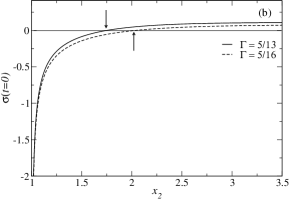
Figure 3: $\sigma_{tot}(t=0)$ as a function of $x_{2}$ for two different values of $\Gamma$: (a) in the metallic regime, for a given fixed $x_{1}=0.1$ and (b) in the insulating regime, for a given fixed $x_{1}=1.0$, and two different values of $\Gamma$, showing how the cutoff for the positivity of density depends on disorder.

In figure 3a, $\sigma(t=0)$ is plotted as a function of $x_{2}$ for two different values of $\Gamma$ in the metallic regime for a fixed $x_{1}=0.1$, while Fig. 3b shows the same in the insulating regime for a fixed $x_{1}=1.0$. From this figure 3b we can see how the increase in disorder (decrease in $\Gamma$) increases the cutoff for $x_{2}$ that ensures the positivity of the density. Fig. 4 shows several numerically evaluated roots $x_{2}=x_{r}$ of $\sigma(t=0)$. For comparison with Eq. (61), we plot the scaled quantities $(\Gamma x_{r})^{2}$ as a function of $(\Gamma x_{1})^{2}$ which, according to Eq. (61), should be a straight line in the metallic regime. Figure 4 shows that the metallic limit agrees very well with Eq. (61), and that the same equation provides a good estimate and an upper bound in the crossover and insulating regimes as well. Nevertheless, in our numerical evaluations, for each $x_{1}$, we will find the value of $x_{r}$ numerically by evaluating the total density at $t=0$. Because of the cutoff in $x_{2}$ at $x_{r}$, $P(g)$ will be given by

$$P(g)=\int_{0}^{\infty}dx_{1}\int_{x_{r}}^{\infty}dx_{2}e^{-S(x_{1},x_{2})}.$$ (63)

Note that since we used the variable $x$ instead of $\lambda$, the action $S(x_{1},x_{2})$ will contain appropriate Jacobian terms.

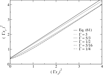
Figure 4: Values of $x_{2}=x_{r}$ for which $\sigma_{tot}(t=0)$ scaled by $\Gamma$ plotted as a function of $(\Gamma x_{1})^{2}$ for several $\Gamma$ in the metallic, insulating and crossover regimes. Eq. (61) fits the metallic regime well, and is a good estimate and an upper bound for the insulating and crossover regions.

The inequalities (61, 62) show that the separation between $x_{1}$ and $x_{2}$ increases with decreasing $\Gamma$. Since $\Gamma\gg 1$ describes metals and $\Gamma\ll 1$ describes insulators, this gives rise to the well-known qualitative picture that all eigenvalues in metals are close to the origin while they are all large and well-separated in the insulating regime. In addition, Eqs. (61) and (62) suggest two more qualitatively distinct regions involving rare but allowed configurations:

(i) $\Gamma\gg 1$, $x_{1}\gg 1$, $x_{2}\gg 1$, but $x_{2}\approx x_{1}$. We will show in this paper that even for metals, this gives rise to the existence of long tails in $P(g)$ in the region $g\ll 1$ (Sec. 5).

(ii) $\Gamma\ll 1$, $x_{1}\ll 1$, $x_{2}\gg 1$. In this insulating region a Gaussian cut off in the log-normal conductance distribution for $g>1$ was found in [1] (Sec. 6).

Thus the qualitative features of the density provide us with much insight, not only about various approximations and their limitations, but also suggesting rare but allowed configurations giving rise to novel possibilities in the distribution.

4.2 Fluctuation correction to the functional integral

As we have seen, the generalized density $\sigma(t)$ goes to zero at $t=0$. This means that the saddle point evaluation of the functional integration over the density requires corrections. The fluctuation correction will involve the integral

$$I_{\sigma}=\int D[\sigma]\exp\left[-\frac{1}{2}\int_{0}^{\infty}dt\int_{0}^{\infty}ds\delta\sigma(t)u(t,s)\delta\sigma(s)\right]$$ (64)

where $u(s,t)$ includes the two body terms, and $\delta\sigma=\sigma-\sigma_{sp}$. The result is in general of the form $I_{\sigma}\sim 1/\sqrt{det|u(t,s)|}.$ This will give rise to a contribution to the free energy of the form $\delta F=+\frac{1}{2}\ln(det|u|).$ Although it should be possible to evaluate the determinant numerically, we can already argue that the correction is usually negligible (see Appendix C). The fluctuation correction to the free energy is relevant only in the extreme metallic regime and it is given by

$$\delta F\approx\frac{1}{2}\ln\lambda_{d}.$$ (65)

4.3 The partial free energies

The partial free energies related with $\sigma_{z}$ and $\sigma_{u1}$ given by Eq. (48) are calculated exactly for any regime. In particular, $F_{zz}$ is relevant for the calculation of the exact variance in the metallic regime as well as to see the qualitative change in the solutions for large and small $x_{2}$:

$$F_{zz}=-\frac{z^{2}}{\beta}\frac{1}{\sinh^{2}(2x_{2})}\left[\frac{1}{3}-\frac{1}{4x^{2}_{2}}+\frac{1}{\sinh^{2}2x_{2}}\right]\;\;\;.$$ (66)

There are also two direct terms

$$F^{0}_{1}=\frac{\beta}{2}\Gamma x^{2}_{1}-\frac{1}{2}\ln(x_{1}\sinh(2x_{1}));\;\;\;F^{z}_{1}=\frac{z}{\cosh^{2}x_{1}},$$ (67)

and the contribution from the fluctuation correction to the functional integral $\delta F$ (65) valid for $x_{2}\ll 1$. Other free energy terms can be calculated within the same approximations as used for the densities (see Appendix B for details). In particular, the free energies can be obtained analytically in the metallic and insulating regimes, keeping the leading orders in $x_{2}$. On the other hand, we will see later that an interesting crossover regime on the insulating side will be determined by the case where $x_{2}\gg 1$, but $x_{1}$ can be arbitrary. Free energy expressions in this regime can also be obtained approximately analytically. Note also that these expressions will be valid for $\beta\neq 2$ as well, for which there will be additional $V_{j}$ terms and therefore additional free energy terms. For quantitative results on $P(g)$, we will integrate numerically Eq. (48) to obtain the free energy.

In the final saddle point action, we have written the total free energy in the form given in (50). Remembering a factor of two for symmetrical terms $F_{ab}=F_{ba}$ for $b\neq a$, we then have

$$F^{0} = F_{\Gamma\Gamma}+F_{u_{1}u_{1}}+F_{u_{2}u_{2}}+F^{0}_{1}+\delta F+2[F_{u_{1}\Gamma}+F_{\Gamma u_{2}}+F^{\Gamma}_{2\Gamma}+F_{u_{1}u_{2}}],$$ (68)

$$F^{\prime} = \frac{1}{z}F^{z}_{1}+\frac{2}{z}[F_{\Gamma z}+F_{zu_{1}}+F_{zu_{2}}+F_{z2}+F^{z}_{2\Gamma}],$$ (69)

$$F^{\prime\prime} = \frac{2}{z^{2}}F_{zz}.$$ (70)

Given the free energies, the action $S$ determines the full distribution $P(g)$. We will discuss several quantitative results in the metallic and deeply insulating regimes as well as qualitative results in the insulating side of the crossover regime analytically. The distribution in the crossover regime has to be obtained numerically.

5 The metallic regime

The metallic regime is characterized by $x_{2}\ll 1$ and the Free energy terms in this regime can be obtained analytically by expanding the potentials (46). Details of the calculations are given In Appendix B.

5.1 Free energy in the metallic limit:

Using $x_{1}<x_{2}\ll 1$ and therefore $\sqrt{\lambda_{d}}\approx\sqrt{x^{2}_{2}-x^{2}_{1}}$, the total free energy in the metallic limit is given by

$$F^{0} \approx a_{1}\Gamma^{2}x^{2}_{2}+a_{2}\ln(x^{2}_{2}-x^{2}_{1})-a_{3}\Gamma\sqrt{x^{2}_{2}-x^{2}_{1}}-\ln x_{1},$$ (71)

$$F^{\prime} \approx \Gamma-b_{1}\Gamma x^{2}_{2}+b_{2}\sqrt{x^{2}_{2}-x^{2}_{1}};\;\;\;\;F^{\prime\prime}\approx-\frac{1}{15},$$ (72)

where $a_{1}=3\pi^{2}/8$, $a_{2}=3/2$, $a_{3}=2\pi$, $b_{1}=2/3+2\left(8-2\zeta(2)-3\zeta(3)\right)/\pi^{2}$ and $b_{2}=32/\pi^{3}$, where $\zeta(n)$ is the Riemann zeta function.

5.2 Saddle point analysis in the deep metallic limit

Since $x_{2}\ll 1$, and $\Gamma\gg 1$, we will keep only the dominant first term in $F^{\prime}$ for the purpose of obtaining a saddle point solution (we will see that $x_{2}$ is $O(1/\Gamma)$, so that the neglected terms are smaller by a factor $1/\Gamma^{2}$ compared to the leading term ). In terms of the scaled variables $\mu\equiv\Gamma\sqrt{x^{2}_{2}-x^{2}_{1}}$ and $\nu\equiv\Gamma x_{1}$, the free energy in this limit is

$$F^{0}\approx a_{1}(\mu^{2}+\nu^{2})+2a_{2}\ln\mu-a_{3}\mu-\ln\nu-\ln\mu+\frac{1}{2}\ln(\mu^{2}+\nu^{2}),$$ (73)

$$F^{\prime}\approx\Gamma;\;\;\;\;F^{\prime\prime}=-\frac{1}{15}.$$ (74)

The last two terms in $F^{0}$ comes from the Jacobian of transformation $dx_{2}=\mu d\mu/(\Gamma\sqrt{\mu^{2}+\nu^{2}})$. Using (52), the solutions to the saddle point equations $\partial S/\partial\mu=\partial S/\partial\nu=0$ are given by

$$\frac{1}{\nu^{2}}=\frac{\mu a_{3}-2a_{2}+1}{\mu^{2}};\;\;\;\;\frac{1}{\mu^{2}+\nu^{2}}=-2a_{1}+\frac{1}{\nu^{2}}.$$ (75)

Eliminating $\nu$ we obtain a cubic equation for $\mu$, whose real solution turns out to be less than the cutoff due to the positivity of the density. This means that the metallic solution is dominated by the boundary value $\mu=\Gamma\sqrt{x^{2}_{2}-x^{2}_{1}}=2/\pi$. The corresponding $\nu=\mu/\sqrt{2}$. Thus the saddle point analysis gives both $x_{1}$ and $x_{2}$ to be of order $1/\Gamma$.

5.3 Correction to $\langle g\rangle$ in the metallic limit

The nth moment of $P(g)$ can be obtained from Eqs. (54) and (55). The average conductance in the metallic limit is $\Gamma$ with leading correction $\sim 1/\Gamma$, for $\beta=2$, with a coefficient obtained exactly in [14]. In order to compare with [14], we write $\langle g\rangle$ as

$$\langle g\rangle=\frac{\int_{0}^{\infty}dx_{1}\int_{x_{r}}^{\infty}dx_{2}\int_{0}^{\infty}dg[(g-F^{\prime})+F^{\prime}]e^{-S}}{\int_{0}^{\infty}dx_{1}\int_{x_{r}}^{\infty}dx_{2}\int_{0}^{\infty}dge^{-S}}.$$ (76)

The first integral over $g$ in the numerator can be done simply, and we write

$$\int_{0}^{\infty}dg[(g-F^{\prime})+F^{\prime}]e^{-S}=|F^{\prime\prime}|e^{-\frac{F^{\prime 2}}{2|F^{\prime\prime}|}-F^{0}}+F^{\prime}\int_{0}^{\infty}dge^{-\frac{(g-F^{\prime})^{2}}{2|F^{\prime\prime}|}-F^{0}}.$$ (77)

In the metallic regime, $F^{\prime}\sim\Gamma\gg 1$, and $|F^{\prime\prime}|=1/15\ll 1$; the first term in (77) is exponentially small and we neglect it. The numerator and the denominator in (76) then have the same integral over $g$. For $F^{\prime}\sim\Gamma\gg 1$, this integral depends on $|F^{\prime\prime}|$ only. Since $|F^{\prime\prime}|$ is a constant, it cancels out from the ratio and we have

$$\langle g\rangle\approx\frac{\int_{0}^{\infty}dx_{1}\int_{x_{r}}^{\infty}dx_{2}F^{\prime}e^{-F^{0}}}{\int_{0}^{\infty}dx_{1}\int_{x_{r}}^{\infty}dx_{2}e^{-F^{0}}}.$$ (78)

The leading term in $F^{\prime}$ is $\Gamma$, independent of $x_{1}$, $x_{2}$, so the leading term for the average conductance is simply $\Gamma$. Scaling $\bar{x}_{i}=x_{i}\Gamma$, we write

$$\langle g\rangle=\Gamma-\frac{\eta}{\Gamma}$$ (79)

where

$$\eta\approx\frac{\int_{0}^{\infty}d\bar{x}_{1}\int_{\bar{x}_{r}}^{\infty}d\bar{x}_{2}\left[b_{1}\bar{x}^{2}_{2}-b_{2}\sqrt{\bar{x}^{2}_{2}-\bar{x}^{2}_{1}}\right]e^{-\bar{F}^{0}}}{\int_{0}^{\infty}d\bar{x}_{1}\int_{\bar{x}_{r}}^{\infty}d\bar{x}_{2}e^{-\bar{F}^{0}}},$$ (80)

$$\bar{F}^{0}=a_{1}\bar{x}^{2}_{2}+a_{2}\ln(\bar{x}^{2}_{2}-\bar{x}^{2}_{1})-a_{3}\sqrt{\bar{x}^{2}_{2}-\bar{x}^{2}_{1}}-\ln\bar{x}_{1},$$ (81)

and $\bar{x}_{r}=\sqrt{\bar{x}^{2}_{1}+(2/\pi)^{2}}$. Note that while the free energy expressions are valid only for $x_{i}\ll 1$, the scaled variables $\bar{x}_{i}$ can be very large. However, the results become insensitive to the upper limit beyond 4. Setting the upper limit at 4 and doing the integral numerically we get

$$\eta=.027$$ (82)

compared to the exact result $\eta=1/45\approx.022$. This shows that our results are good in the metallic limit up to order $1/\Gamma$. This is consistent with the fact that $x_{i}\sim 1/\Gamma,(i=1,2)$, and that we kept only terms up to order $x_{i}$ and $\Gamma x^{2}_{i}$ in Eqs. (71, 72).

5.4 Variance in the metallic limit

Using $g^{2}=(g-F^{\prime})^{2}+2gF^{\prime}-F^{\prime 2}$, and the above approximation that $F^{\prime 2}/2|F^{\prime\prime}|\gg 1$ with $F^{\prime\prime}$ constant, we can write the second moment, following the same procedure as above, as $\langle g^{2}\rangle=\langle|F^{\prime\prime}|+F^{\prime 2}\rangle$. Then the variance is simply

$$var(g)=\langle g^{2}\rangle-(\langle g\rangle)^{2}=|F^{\prime\prime}|=\frac{1}{15},$$ (83)

which is the correct variance in the metallic limit. We do not calculate the correction to the variance for $\beta=2$, because the leading correction is of order $1/\Gamma^{2}$, and our approximate free energy expressions are not good up to this order in the metallic regime. However, the leading correction for $\beta\neq 2$ is of order $1/\Gamma$, and we will see later that our approximations yield values very close to the exact result.

More generally, we can evaluate the integrals $J_{k}$ defined in (55) numerically and obtain the average and variance of $g$ as a function of the disorder parameter $\Gamma$. Results of these calculations have been reported in [2]. They are in very good agreement with the exact results in the metallic region.

5.5 Conductance distribution in the metallic limit

The saddle point analysis of the metallic regime gives both $x_{1}$ and $x_{2}$ of order $1/\Gamma$, which justifies keeping only the leading term in $F^{\prime}$ in Eq. (72), namely $F^{\prime}=\Gamma$, deep in the metallic regime. Then the distribution $P(g)$ becomes trivial, because the $g$-dependent part can be taken out of the integrals over $x_{1}$ and $x_{2}$ and the integrals only give the normalization factor. We obtain the known Gaussian distribution:

$$P(g)\propto e^{-\frac{15}{2}(g-\Gamma)^{2}},$$ (84)

with mean $\langle g\rangle=\Gamma$ and $var(g)=1/15$. Using Eqs. (71, 72), $P(g)$ can be directly obtained by numerical integration. As an example, Fig. 5 shows the result of the numerical integration for $\Gamma=2$, compared with Eq. (84) appropriately normalized.

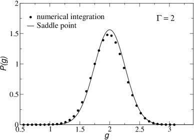
Figure 5: Gaussian distribution of the conductance in the metallic regime numerically obtained from Eqs. (71) and (72) for $\Gamma=2$, compared with the saddle point result Eq. (84).

5.6 $P(g)$ for $g\ll 1$ in the metallic limit

An important question for the metallic distribution is whether there are long (non-Gaussian) tails for $g\ll 1$. These will signal rare events (localized states) dominating the tail of the distribution, as suggested by field-theory models [11]. With appropriate approximations of our free energy, we can analytically consider this region qualitatively. We will be interested only in $g\ll 1$, which can happen only if $x_{1}\gg 1$ and $x_{2}\gg 1$. However, metal means large $\Gamma$, and the positivity of the density requires that $x^{2}_{2}-x^{2}_{1}>4/\pi^{2}\Gamma^{2}$, Eq. (61). This means that $x_{2}$ can be very close to $x_{1}$ (in contrast, for the insulating case, $\Gamma\ll 1$, and $x_{2}\gg x_{1}$).

The free energy in the limit $x_{2}\gg 1$ can be written as

$$F^{0}\approx 2\Gamma^{2}x^{2}_{2}-6\Gamma x_{2}+\Gamma x^{2}_{1}-\frac{1}{2}\ln(x_{1}\sinh(2x_{1}));$$ (85)

$$F^{\prime}\approx\frac{1}{\cosh^{2}x_{1}}+\frac{2\Gamma}{\sinh 2x_{2}};\;\;\;F^{\prime\prime}\approx-\frac{4}{3}e^{-4x_{2}}.$$ (86)

The saddle point solution is given by

$$\frac{\partial S}{\partial x_{1}}=\frac{2(g-F^{\prime})}{2|F^{\prime\prime}|}\left(-\frac{\partial F^{\prime}}{\partial x_{1}}\right)+\frac{\partial F^{0}}{\partial x_{1}}=0.$$ (87)

Since the quantity $1/|F^{\prime\prime}|$ is exponentially large, the saddle point solution is given simply by putting its coefficient equal to zero, i.e. $g=F^{\prime}+O(e^{-4x_{2}})$.

For both $x_{1}\gg 1$ and $x_{2}\gg 1$ but $x_{2}\approx x_{1}$ and $\Gamma\gg 1$, the second term in $F^{\prime}$ can become the dominant term (the first term dominates for $x_{2}\gg x_{1}\gg 1$ and $\Gamma\ll 1$ which will describe the insulating region, and also for $x_{1}\ll 1$ and $\Gamma\approx 1$ which will describe the crossover region). Then the saddle point solution for $x_{2}$ gives $g=2\Gamma/\sinh 2x_{2}$. The leading order solution is $x_{2}\approx\frac{1}{2}\ln(4\Gamma/g),$ leading to

$$P(g)\propto e^{-2\langle g\rangle^{2}\left(\ln\frac{4\langle g\rangle}{g}-\frac{3}{2\langle g\rangle}\right)^{2}};\;\;\;g\ll 1,\;\;\;\langle g\rangle\gg 1,$$ (88)

where we have used the fact that in the metallic limit $\langle g\rangle=\Gamma$. The fluctuation correction does not add any further $g$ dependence.

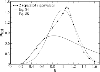
Figure 6: $P(g)$ for $\Gamma=1.0$ obtained in [2] compared with normalized (88) (solid line) and normalized (84) (dashed line). The log-normal tail of the distribution for $g\ll 1$ is clearly distinguishable from the Gaussian tail. Note that $\Gamma=1.0$ is slightly beyond the metallic regime (a larger value would be metallic) where (84) is not strictly valid. Nevertheless, it clearly shows the Gaussian tail in the $g\gg 1$ limit as expected for a metal but a log-normal tail in the $g\ll 1$ limit.

Figure 6 shows $P(g)$ given by Eq. (88) compared with the distribution of $g$ calculated from the two separated eigenvalue case for $\Gamma=1.0$, as well as the Gaussian tail expected from Eq. (84). Note that $\Gamma=1.0$ is slightly beyond the metallic regime (a larger value of $\Gamma$ would be metallic). Nevertheless it clearly shows the existence of a log-normal tail in the $g\ll 1$ regime compared to a Gaussian tail in the $g\gg 1$ regime for the same value of $\Gamma$ close to the metallic limit.

6 The insulating and crossover regimes within the one separated eigenvalue approximation

As emphasized in [2, 3], we need to isolate at least two eigenvalues in order to study the insulating and the crossover regimes. This we will do later. On the other hand, the one-eigenvalue framework allows us to obtain many analytical results, which helps us to better understand the qualitative nature of the solutions. We will therefore expect our results in this section to be valid only qualitatively. In particular, we will point out why the one eigenvalue separation fails very close to $g=1$ even qualitatively. In all other cases the numerical evaluations with two separated eigenvalues improve the one eigenvalue results quantitatively, without changing them qualitatively.

6.1 Free energy and saddle point solution in the insulating limit

In the limit $\Gamma\ll 1$ and $x_{2}\gg x_{1}\gg 1$, the free energy simplifies to

$$F^{0}\approx 2\Gamma^{2}x^{2}_{2}-6\Gamma x_{2}+\Gamma x^{2}_{1}-x_{1}$$ (89)

$$F^{\prime}\approx 4e^{-2x_{1}};\;\;\;F^{\prime\prime}\approx-\frac{4}{3}e^{-4x_{2}}.$$ (90)

As before, since $x_{2}\gg 1$, the saddle point solution is given by putting $g=F^{\prime}+O(e^{-4x_{2}})=4e^{-2x_{1}}$, so that $x_{1sp}=-\frac{1}{2}\ln u$, $u=g/4$. The saddle point value of $x_{2}$ is obtained from

$$\frac{\partial S}{\partial x_{2}}=3e^{4x_{2}}(g-F^{\prime})^{2}+\frac{\partial F^{0}}{\partial x_{2}}=\frac{\partial F^{0}}{\partial x_{2}}+O(e^{-4x_{2}})=0.$$ (91)

This gives $x_{2sp}=3/2\Gamma$, independent of $g$. As we will see (Eq. 95), since $x_{1sp}=-\ln u/2$, $x_{1sp}\sim 1/2\Gamma$, so $x_{2sp}\gg x_{1sp}$ for $\Gamma\ll 1$.

6.2 Conductance distribution in the insulating limit

Since $x_{2sp}$ is independent of $g$, it only contributes to the normalization constant. The distribution of conductance in saddle point approximation is determined by $x_{1}$ only,

$$P_{sp}(g)\propto e^{-(-x_{1}+\Gamma x^{2}_{1})}\propto e^{-\frac{\Gamma}{4}(\ln u+1/\Gamma)^{2}}.$$ (92)

To this we need to add the fluctuation correction around the saddle point $P(g)\propto e^{-S_{sp}}/\sqrt{|S^{\prime\prime}|}$, where

$$S^{\prime\prime}=\frac{\partial^{2}S}{\partial x^{2}_{1}}=\frac{g-F^{\prime}}{|F^{\prime\prime}|}\left(-\frac{\partial^{2}F^{\prime}}{\partial x^{2}_{1}}\right)+\frac{1}{|F^{\prime\prime}|}\left(\frac{\partial F^{\prime}}{\partial x_{1}}\right)^{2}+\frac{\partial^{2}F^{0}}{\partial x^{2}_{1}}.$$ (93)

The first term is zero at the saddle point. The third term is negligible compared to the exponentially large second term, which gives $S^{\prime\prime}(x_{sp})\propto g^{2}.$ The distribution of $\ln g$ can then be written as

$$P(\ln g)=P(g)\frac{dg}{d\ln g}=gP(g)\propto e^{-\frac{\Gamma}{4}(\ln(g/4)+1/\Gamma)^{2}}.$$ (94)

This is a log-normal distribution with mean and variance given by

$$\langle-\ln(g/4)\rangle=\frac{1}{\Gamma};\;\;\;var(\ln(g/4))=\frac{2}{\Gamma},$$ (95)

which agrees with known results.

6.3 Mean and variance of $g$ as function of $\Gamma$

In the insulating limit, the density is zero, and the calculation of the mean and the variance becomes simple. In the crossover regime, one can use the full free energy to numerically obtain the mean and the variance using (54-56). These two moments of $P(g)$ have been reported earlier in [2] and compared with exact result. They fail in the crossover regime, but the two separated eigenvalue approximation substantially improves the agreement with exact results both in the insulating and in the crossover regimes.

6.4 Distribution in the crossover regime

To obtain quantitative results in the crossover regime, we will need to obtain the free energy terms by numerically evaluating Eq. (51). However, the regime $x_{2}\gg 1$, $x_{1}\ll 1$, corresponds to $\Gamma$$\stackrel{{\scriptstyle<}}{{\sim}}$1 which characterizes the crossover regime from the insulating side. For this case, the free energy contributions are the same as in Eqs. (89,90). This time, however, the fact that $x_{2}\gg x_{1}$ makes the first term in $F^{\prime}$ dominate. The results have been discussed in [1], where a ‘one-sided log-normal distribution’ with sharp features in $P(g)$ at $g=1$ was predicted. Here as an example, we show in Fig. 7 the distribution $P(g)$ for $\Gamma=5/12$ calculated by using the results in [1]. On the other hand, note that the region $\Gamma$ $\stackrel{{\scriptstyle>}}{{\sim}}$1, which corresponds to the crossover regime from the metallic side, is characterized by $x_{2}\sim 1$, $x_{1}\ll 1$. Our approximate free energies are not valid in this regime.

The saddle point solution of $x_{1}$ is again given by $g=F^{\prime}$ and we have $\cosh x_{1}=\frac{1}{\sqrt{g}}$. Note that since $\cosh x_{1}\geq 1$, the boundary of the saddle point solution is given by $g\leq 1$. It is the existence of this boundary that makes the current solution fail very close to $g=1$. The two separated eigenvalue framework reveals the existence of a non-analyticity in the distribution near this point [3].

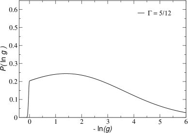
Figure 7: The ‘one-sided log-normal distribution’ of the conductance in the crossover regime from the insulating side, where sharp features in the distribution were found around g=1 [1].

7 Separating out two eigenvalues

As mentioned earlier, the two separated eigenvalue case has been treated in [2, 3]. Here we give a summary for completeness. Separating out 2 eigenvalues simply means that equation (12) for $H_{1}$ is now replaced by

$$H_{1,2}=\sum_{i\geq 3}u(x_{i},x_{1})+\sum_{i\geq 3}u(x_{i},x_{2})+u(x_{1},x_{2})+V(x_{1})+V(x_{2}).$$ (96)

The continuum approximation (17) now becomes

$$H(x_{1},x_{2},x_{3};\sigma(x))=V(x_{1})+V(x_{2})+u(x_{1},x_{2})+\int_{x_{3}}^{b}dx\sigma(x)u(x,x_{1})$$

$$+\int_{x_{3}}^{b}dx\sigma(x)u(x,x_{2})+\frac{1}{2}\int_{x_{3}}^{b}dx\int_{x_{3}}^{b}dx^{\prime}\sigma(x)u(x,x^{\prime})\sigma(x^{\prime})+\int_{x_{2}}^{b}dx\sigma(x)V_{\Gamma}(x),$$

while Eq. (20) for the free energy is now

$$F(x_{1},x_{2},x_{3};\sigma(x))=\beta H(x_{1},x_{2},x_{3};\sigma(x))+\frac{i\tau}{\cosh^{2}x_{1}}+\frac{i\tau}{\cosh^{2}x_{2}}+i\tau\int_{x_{3}}^{\infty}\frac{\sigma(x)}{\cosh^{2}x},$$ (98)

and the distribution $P(g)$ becomes

$$P(g)=\frac{1}{Z}\int_{-\infty}^{\infty}\frac{d\tau}{2\pi}\e^{i\tau g}\int_{0}^{\infty}dx_{1}\int_{x_{1}}^{\infty}dx_{2}\int_{x_{2}}^{\infty}dx_{3}\int D[\sigma(x)]\e^{-F(x_{1},x_{2},x_{3};\sigma(x))}.$$ (99)

The shift parameter in (28) is now $\lambda_{3}$ and $V_{tot}$ Eq. (45) has two additional terms

$$V_{tot}(\eta(t)+\lambda_{3})=V_{\Gamma}+V_{u_{11}}+V_{u_{21}}++V_{u_{12}}+V_{u_{22}}+V_{z}$$ (100)

with corresponding densities $\sigma(t)=\sigma_{\Gamma}+\sigma_{u_{11}}+\sigma_{u_{21}}+\sigma_{u_{12}}+\sigma_{u_{22}}+\sigma_{z}$. Here $V_{u_{11}}$ and $V_{u_{12}}$ are just the old $V_{u_{1}}$ and $V_{u_{2}}$ with shift parameter $\lambda_{2}$ replaced by $\lambda_{3}$, (similarly for $\sigma_{u_{11}}$ and $\sigma_{u_{12}}$). The new terms $V_{u_{21}}$ and $V_{u_{22}}$ can be written down following the substitution

$$V_{u_{21}}=V_{u_{1}}(\lambda_{2}\rightarrow\lambda_{3},\lambda_{1}\rightarrow\lambda_{2});\;\;\;V_{u_{22}}=V_{u_{2}}(\lambda_{2}\rightarrow\lambda_{3},\lambda_{1}\rightarrow\lambda_{2}),$$ (101)

and similarly for $\sigma_{u_{21}}$ and $\sigma_{u_{22}}$. In terms of the new saddle point densities and free energies, the expression for $P(g)$ is similar to (51), with one extra integral over $\lambda_{3}$:

$$P(g)=\frac{1}{Z}\int_{0}^{\infty}d\lambda_{1}\int_{\lambda_{1}}^{\infty}d\lambda_{2}\int_{\lambda_{2}}^{\infty}d\lambda_{3}e^{-S}$$ (102)

where the action $S$ has the same form as (52). The mean and the variance can be obtained from the integrals $J_{k}$ of (56), now given by

$$J_{k}=\int_{0}^{\infty}dx_{1}\int_{x_{1}}^{\infty}dx_{2}\int_{x_{3}}^{\infty}dx_{2}e^{-F^{0}}I_{k}(x_{1},x_{2},x_{3}).$$ (103)

The extra integral over $\lambda_{3}$ makes analytical calculations of $P(g)$ difficult. Even numerical evaluations become involved. We will not only put $V_{2}=0$ as discussed before, but also keep only the interaction between nearest $\lambda$’s, neglecting in the potential terms the argument $\lambda_{1}$ compared to $\lambda_{3}$. Thus e.g. we set

$$V_{u_{11}}\approx-\frac{1}{2}\ln(\sinh^{2}t+\lambda_{3})$$ (104)

Since $\lambda_{3}\gg\lambda_{1}$ beyond the metallic regime, this is a valid approximation in the regimes we are interested in.

The rest of the calculations are exactly as discussed for the one eigenvalue case. For example, the density again becomes negative for sufficiently small $x_{3}-x_{2}$. The positivity of the density is guaranteed by numerically obtaining the minimum value of $x_{3}$ for which the density is zero at its minimum.

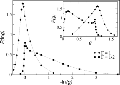
Figure 8: Distribution of the conductance in the crossover regime. A broad distribution is found for $\Gamma=1/2$ (squares); eventually $P(\ln g)$ goes to the log-normal distribution in the insulating regime. For $\Gamma=1$ (diamonds) $P(g)$ is closer to the Gaussian distribution (inset, from [2]) which is expected in the metallic regime.

It is straightforward to repeat the evaluations for the mean and the variance of $g$ as functions of $\Gamma$ within the two separated eigenvalue framework in the crossover regime, and in the insulating regime where the density is put equal to zero. These results have been reported before [2] and shows that they are much better than the one eigenvalue case. In particular the variance now follows the non trivial hump at $\Gamma=1/2$ in the exact result [14]. Details of the results for $P(g)$ in the crossover regime have also been reported in [2]. They compare well with numerical results available [9], including the direct Monte Carlo evaluation of Eq. (8) [27]. As an example of the results obtained by separating out two eigenvalues, we show in figure 8 the distribution of the conductance as a function of $\ln g$ and $g$ (inset) in the crossover region. For $\Gamma=1/2$, a broad distribution is observed, as reported in numerical studies. On the other hand, $P(\ln g)$ goes, eventually in the insulating regime, to a log-normal distribution (as the one shown in Fig. 7). For $\Gamma=1$, which is closer to the metallic regime, the profile of $P(g)$ is close to a Gaussian distribution, as expected.

Note that in our derivation for the distribution in the crossover region within the one separated eigenvalue framework, the saddle point solution existed only on one side of $g=1$ while the other side was dominated by the boundary value. Separating out two eigenvalues allows us to treat the case near $g=1$ with more accuracy. As discussed in [3], we obtain a discontinuity in $P^{\prime}(g)=dP(g)/dg$ at $g=1+\alpha$ where $\alpha=1/\cosh^{2}(3/2\Gamma)$ with $P^{\prime}\sim e^{-2/\Gamma}$ for $g\geq 1+\alpha$ and with an almost flat distribution for $g<1+\alpha$. In figure 9 we show $P(g)$ and its derivative (inset) around $g=1$ for two different values of disorder, both in the insulating regime, illustrating the discontinuity close to $g=1$ reported in [3] and observed in numerical analysis [7].

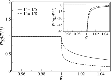
Figure 9: $P(g)$ and its derivative $P^{\prime}(g)$ (inset) around $g=1$ in the insulating regime. The discontinuity in $P(g)$ is at $g=1+\alpha$ [3]. Here $\alpha\sim 10^{-6}$ ($10^{-8}$) for $\Gamma=1/5$ ($\Gamma=1/8$).

8 The case $\beta\neq 2$

In this section we come back to our simpler one separated eigenvalue approximation. As in section 2, we will use the metallic limit Eq. (5) to be true for all regimes. Then the shift approximation and the corresponding expression for density carries through, the only difference is that there are three additional terms to be added to the $V_{tot}$, defined in (24). One is obtained from the last term in (15), while considering the continuum approximation: rewriting this last term in the $\lambda$ variable, using $\lambda=\sinh^{2}x$, and then doing the change of variable $\sinh t=\lambda-\lambda_{2}$, as in Eq. (34), we have

$$V^{\alpha}_{0}(t)=\alpha[\ln({\rm arsinh}^{2}\sqrt{\sinh^{2}t+\lambda_{2}})+\ln(\sinh^{2}t+\lambda_{2})+\ln(\cosh^{2}t+\lambda_{2})].$$ (105)

The same last term in (15) also gives a direct term from the separation of the lowest level,

$$V^{\alpha}_{1}(x_{1})=2\alpha\ln(x_{1}\sinh(2x_{1})).$$ (106)

A third term comes from the ‘entropy’ term of Dyson [24] derived as the second term in (23)

$$V^{\alpha}_{2}(t)=-4\alpha\ln\sigma(t).$$ (107)

It is normally assumed that this term does not change the density appreciably, so the density appearing in (44) can be taken to be the density due to the other terms. However, it includes $\sigma_{z}$, and therefore the free energy is no longer quadratic in $z$. This means that instead of doing the $\tau$ integral exactly analytically, we have to do it either numerically, or try for a saddle point solution. On the other hand, since the largest density in the metallic regime is $\sigma_{\Gamma}$, we can expand the logarithm and keep only the leading term in $z$. As we will see, this will be sufficient to give the leading correction to the variance of $g$ in this regime.

8.1 Correction to the metallic mean conductance

The leading contribution to $F^{\alpha}_{z1}$ determines the leading correction to the mean conductance $\langle g\rangle$. We have

$$F^{\alpha}_{z1}=\frac{\beta}{2}\int dtV_{z}\sigma^{\alpha}_{1},$$ (108)

where the density is obtained from the potential $V^{\alpha}_{1}(t)$, Eq. (105). Comparing with the potentials we already have, we can rewrite it as

$$V^{\alpha}_{1}(t)=-2\alpha\left(V_{u_{2}}|_{x_{1}\rightarrow 0}+V_{u_{1}}|_{\lambda_{d}\rightarrow\lambda_{2}}+V_{u_{1}}|_{\lambda_{d}\rightarrow 1+\lambda_{2}}\right).$$ (109)

Note that the last term is a $\lambda_{d}>1$ term but will contribute in the metallic limit when $\lambda_{2}\ll 1$. Thus the free energy can be written down in terms of known results

$$F^{\alpha}_{z1}=-2\alpha\left(F_{zu_{2}}|_{x_{1}\rightarrow 0}+F_{zu_{1}}|_{\lambda_{d}\rightarrow\lambda_{2}}+F_{zu_{1}}|_{\lambda_{d}\rightarrow 1+\lambda_{2}}\right).$$ (110)

Collecting all the (already known) results, we obtain in the metallic limit

$$F^{\alpha}_{z1}\approx\alpha z\left(\frac{4}{3}-b_{2}x_{2}\right).$$ (111)

Since there is a constant term independent of $x_{i}$ and this contributes to $F^{\prime}$, we immediately get a correction to the average conductance $\Gamma$, given by

$$\langle g\rangle=\Gamma+\alpha\frac{8}{3}=\Gamma+\left(1-\frac{2}{\beta}\right)\frac{1}{3},$$ (112)

where we have included a factor of two for the symmetric term in the free energy. The correction agrees with exact result.

8.2 Correction to the metallic variance of conductance

The leading correction to the variance comes from the contribution to $F^{\alpha z}_{z2}$ from $V^{\alpha}_{2}(t)$, Eq. (107). Note that $\sigma_{\Gamma}$ is the largest term, except very close to $t=0$ in a small range where $\sigma_{u_{1}}$ and $\sigma_{u_{2}}$ become comparable. We neglect this complication, and in order to extract the $z^{2}$ term, take as a first approximation $\sigma(t)\approx\sigma_{\Gamma}(t)+\sigma_{z}(t)$. Then using $\sigma_{\Gamma}(t)\gg\sigma_{z}(t)$, we expand the logarithm, $V^{\alpha}_{2}(t)\approx\ln\sigma_{\Gamma}+\sigma_{z}/\sigma_{\Gamma}$. The first term to leading order will give a constant which we ignore, and a term proportional to $x^{2}_{2}$ in the metallic limit. The second term to leading order would consist of taking the $\lambda_{2}\rightarrow 0$ limit of both the densities. Then we have

$$F^{\alpha z}_{z2}=\frac{\beta}{2}\int dt(-4\alpha)\frac{1}{\Gamma}\sigma_{z};\;\;\;\sigma_{z}=-\frac{8\alpha z^{2}}{\beta\Gamma}\int_{0}^{\infty}dt\left[\frac{\pi^{2}/4-3t^{2}}{(t^{2}+\pi^{2}/4)^{3}}\right]^{2}.$$ (113)

The result of this last integral is $12/\pi^{3}$. Then we have

$$F^{\alpha z}_{z2}=-\frac{1}{2}z^{2}\frac{1}{\beta\Gamma}\left(1-\frac{2}{\beta}\right)\frac{24}{\pi^{6}},$$ (114)

which gives a correction to the variance

$$\delta(var(g))=\frac{1}{\beta\Gamma}\left(1-\frac{2}{\beta}\right)\frac{24}{\pi^{6}}.$$ (115)

The exact result [14] can be written as $\delta(var(g))=\frac{1}{\beta\Gamma}(1-\frac{2}{\beta})\mu$, with $\mu=8/315=0.0254$, while for us, $\mu=24/\pi^{6}=0.0250$, which is very close. The $\beta$ and $\Gamma$ dependence are also correct (in [14], $\zeta/L=2\Gamma$; $\langle g\rangle$ and $var(g)$ have a factor 2 and 4 from spin, respectively).

8.3 The density $\sigma^{\alpha}_{1}$

Since the potential $V^{\alpha}_{1}$ can be written in terms of potential already considered, the corresponding density $\sigma^{\alpha}_{1}$ can also be written down from the known densities, given as

$$\sigma^{\alpha}_{1}(t)=-2\alpha\left(\sigma_{u_{2}}|_{x_{1}\rightarrow 0}+\sigma_{u_{1}}|_{\lambda_{d}\rightarrow\lambda_{2}}+\sigma_{u_{1}}|_{\lambda_{d}\rightarrow 1+\lambda_{2}}\right).$$ (116)

In the metallic limit this simplifies to

$$\sigma^{\alpha}_{1}(t)\approx 8\alpha\left[\frac{1}{4t^{2}+\pi^{2}}+\frac{1}{2\pi}\frac{x_{2}}{t^{2}+x^{2}_{2}}\right],$$ (117)

while in the limit $x_{2}\rightarrow 0$,

$$\sigma^{\alpha}_{1}(t)\rightarrow 8\alpha\left[\frac{1}{4t^{2}+\pi^{2}}+\frac{1}{4}\delta(t-0^{+})\right],$$ (118)

which agrees with [26].

9 Summary and conclusion

Given the distribution of the transmission eigenvalues, we have developed a simple method to obtain the full distribution of conductances $P(g)$ at all strengths of disorder. The method is based on the mapping of the $N$ eigenvalues to an electrostatic problem of $N$ charges on the positive line with one- and two-body interactions. Instead of treating all the charges as part of a continuum in the $N\rightarrow\infty$ limit, we introduce the idea of separating out a finite number of charges close to the origin (corresponding to the most conducting channels) and treating the rest as a continuum. This allows us to treat the strong disorder region as well where the continuum model breaks down due to the large separation between the charges, and where a finite number of discrete charges give a better description. While the set of discrete charges are treated exactly, the continuum part is treated within a saddle point approximation to obtain a saddle point free energy, from which all the relevant transport quantities are evaluated. The saddle point density of the continuum and its relation to the set of discrete charges show how the nature of the solution changes qualitatively with increasing disorder, and allows us to look for rare but allowed configurations that give rise to novel characteristics of the distribution. While two such characteristics, namely the existence of non-analyticity near $g=1$ and the resulting asymmetry in the distribution have been reported earlier, we show here for the first time within the same framework that there exists a log-normal tail in $P(g)$ for $g\ll 1$ even for weak disorder where the average $\langle g\rangle\gg 1$, consistent with earlier field theory calculations. In order to check the accuracy of our method, we also obtain several other results in the metallic limit for which exact results are available. These include the average and the variance of conductance to order $1/\Gamma$ for all symmetry classes and the difference in the saddle point density between different symmetry classes.

The method developed here is very general and can be applied to other quantities as well, e.g. the study of the distribution of shot noise as well as the conductance distribution in the presence of Andreev scattering in an NS (Normal metal-Superconductor) junction.

One should keep in mind that the DMPK approach does not contain the effects of wave function correlations in the transverse direction, which are expected to be important in higher dimensions [28]. Nonetheless, the novel features in $P(g)$ near $g=1$ within our framework appears under very robust conditions which are independent of dimensionality. It is therefore possible that some of the features will persist in higher dimensions as well. The similarities of the shape of $P(g)$ in the crossover regime obtained within the current framework with the numerically determined $P(g)$ in 3D at the critical point appears to be consistent with the above conjecture.

This work has been supported in part by SFB 195 and by the Center for Functional Nanostructures of the der Deutsche Forschungsgemeinschaft. P.W. acknowledges support through a Max-Planck Research Award. V. A. G. is grateful for hospitality at the IPCMS-GEMME, Strasbourg (France) where part of this work was done.

Appendix A Partial densities

In the following we give some details of the calculations for the partial densities mentioned in Sec. 4.

It is convenient to define the integral:

$$\Omega_{a}(q)=\int_{0}^{\infty}ds\sin(qs)\frac{d}{ds}V_{a}(\zeta(s)+\lambda_{2}).$$ (119)

Then the partial density $\sigma_{a}$ is given by

$$\sigma_{a}=\frac{2}{\pi^{2}}\int_{0}^{\infty}dq\cos(qt)(1-e^{-\pi q})\Omega_{a}(q).$$ (120)

• Partial density $\sigma_{z}$:

  Using the above definition with $V_{z}$ given by Eq. (46) we have

  $$\Omega_{z}(q)=\int_{0}^{\infty}ds\sin(qs)\frac{d}{ds}\frac{z}{\cosh^{2}s+\lambda_{2}}$$ (121)

  which can be done by partial integration with result [29]:

  $$\Omega_{z}(q)=-z\frac{\pi}{2}\frac{1}{\sqrt{\lambda_{2}(1+\lambda_{2})}}\frac{q\sin(qa/2)}{\sinh(q\pi/2)}$$ (122)

  where

  $$a={\rm arcosh}(1+2\lambda_{2})=2{\rm arsinh}\sqrt{\lambda_{2}}=2x_{2}.$$ (123)

  Therefore the density $\sigma_{z}$ can be written as

  $$\sigma_{z}(t)=\frac{2}{\pi}\frac{z}{\sqrt{\lambda_{2}(1+\lambda_{2})}}\frac{\partial}{\partial s}\frac{\partial}{\partial\gamma}\int_{0}^{\infty}dq\frac{\sin(qs)}{q}\sin\left(\frac{q2x_{2}}{2}\right)e^{-\gamma q}$$ (124)

  evaluated at $\gamma=\pi/2$. From [29] and after algebraic simplification we obtain $\sigma_{z}$ as given in (59a).

• Partial density $\sigma_{u1}$

  We will first consider the metallic regime. Taking the derivative of $V_{u1}$ we have

  $$\Omega_{u_{1}}=-\frac{1}{2}\int_{0}^{\infty}ds\frac{\sin(qs)\sinh(2s)}{\sinh^{2}s+\lambda_{2}-\lambda_{1}}$$ (125)

  and using $\sinh^{2}s=(\cosh(2s)-1)/2$ then $\Omega_{u_{1}}$ is given by

  $$\Omega_{u_{1}}=-\frac{\pi}{2}\frac{\cosh(qa_{0}/2)}{\sinh(q\pi/2)},\;\;\;{\rm for}\;\lambda_{d}<1,$$ (126)

  where $\lambda_{d}=\lambda_{2}-\lambda_{1}$ and $a_{0}=\pi-2\arcsin\sqrt{\lambda_{d}}$. Finally, after writing $(1-e^{-\pi q})=2e^{-\pi q/2}\sinh(\pi q/2)$ in (A2), $\sigma_{u1}$ can be written as given in (59b) for $\lambda_{d}<1$.

  In order to obtain $\sigma_{u1}$ for $\lambda_{d}>1$, we follow a different method. First we take the derivative w.r.t. $\lambda_{d}$:

  $$\frac{\partial\Omega_{u_{1}}}{\partial\lambda_{d}}=-\frac{1}{2}\int_{0}^{\infty}ds\sin(qs)\frac{d}{ds}\frac{1}{\sinh^{2}s+\lambda_{d}}.$$ (127)

  A partial integration gives the boundary term zero and

  $$\frac{\partial\Omega_{u_{1}}}{\partial\lambda_{d}}=\frac{q}{2}\frac{\partial I_{\Omega_{1}}}{\partial\lambda_{d}}$$ (128)

  where

  $$\frac{\partial I_{\Omega_{1}}}{\partial\lambda_{d}}=2\int_{0}^{\infty}ds\frac{\cos(qs)}{\cosh(2s)+(2\lambda_{d}-1)}.$$ (129)

  For $\lambda_{d}>1$ [29],

  $$\frac{\partial I^{>}_{\Omega_{1}}}{\partial\lambda_{d}}=\frac{\pi}{\sinh(q\pi/2)}\frac{\sin[(q/2){\rm arcosh}(2\lambda_{d}-1)]}{\sqrt{(2\lambda_{d}-1)^{2}-1}}.$$ (130)

  Using ${\rm arcosh}(2\lambda_{d}-1)=y$, we can integrate to obtain

  $$I^{>}_{\Omega_{1}}=-\frac{\pi}{q}\frac{\cos(qy/2)}{\sinh(q\pi/2)}+\textrm{terms independent of }\lambda_{d}.$$ (131)

  Neglecting the $\lambda_{d}$-independent terms, then we have a result valid for $\lambda_{d}>1$. Therefore we have

  $$\Omega_{u_{1}}=-\frac{\pi}{2\sinh(q\pi/2)}\left\{\begin{array}[]{ll}\cosh(qa_{0}/2),&\lambda_{d}<1;\\ \cos(qb_{0}/2),&\lambda_{d}>1;\end{array}\right.$$ (132)

  where we have included the result for $\lambda_{d}<1$ obtained within this method (see Eq. (A8)) and $b_{0}={\rm arcosh}(2\lambda_{d}-1)$. We can check that there is no $\lambda_{d}$ independent terms by comparing the two expressions of $\Omega_{u_{1}}$ at the boundary $\lambda_{d}=1$ i.e. at $a_{0}=0$ and $b_{0}=0$ for $\lambda_{d}<1$ and $\lambda_{d}>1$, respectively. We note that $b_{0}=ia_{0}$, and the expression for $\lambda_{d}<1$ becomes valid for $\lambda_{d}>1$ if we allow $a_{0}$ to be complex. The corresponding $\sigma_{u_{1}}$ for all $\lambda_{d}$ is then given by (59b).

• Partial density $\sigma_{u2}$

  Here we will use our approximation to $V^{\prime}_{u2}(s)$, Eq. (58). This approximation starts to fail for $x_{2}>5$ and/or $x_{d}\ll 1$, however the metallic limit $x_{2}\to 0$ is well described and also it has been shown in [2] that this approximation remains valid in the crossover regime. Equation (58) can also be written as

  $$V^{\prime}_{u_{2}}(s)\approx\frac{s}{2}\left[\frac{1}{(s-ic)^{2}+\beta^{2}_{1}}+\frac{1}{(s+ic)^{2}+\beta^{2}_{1}}\right]-\frac{as^{2}_{m}s}{(s^{2}+s^{2}_{m})^{2}+4c^{2}s^{2}}$$ (133)

  with $\beta_{1}^{2}=c^{2}+s_{m}^{2}$. Introducing this expression in (A1), we get

  $$\Omega_{u_{2}}(q)\approx-\frac{\partial}{\partial q}\int_{0}^{\infty}\frac{ds}{s}\cos(qs)V^{\prime}_{u_{2}}(s)=-\frac{\pi}{4\beta_{1}}\left[A_{+}e^{-q(\beta_{1}+c)}+A_{-}e^{-q(\beta_{1}-c)}\right]$$ (134)

  where $A_{\pm}=\beta_{1}\pm c\pm as^{2}_{m}/2c$, and the corresponding density becomes as given in (59c).

• Partial density $\sigma_{\Gamma}$

  In order to obtain $\sigma_{\Gamma}$ we will use our approximation to $V^{\prime}_{\Gamma}(s)$, Eq. (57). In this case, we have

  $$\Omega_{\Gamma} \approx \Gamma\int_{0}^{\infty}ds\sin(qs)s\left[1-\frac{a_{4}}{\cosh(2s)+\cosh\delta_{1}}\right]$$ (135)

  $$= -\pi\delta^{\prime}(q)+a_{4}\frac{\partial}{\partial q}\int_{0}^{\infty}ds\frac{\cos(qs)}{\cosh(2s)+\cosh\delta_{1}}$$

  $$= -\pi\delta^{\prime}(q)+a_{4}\frac{\pi}{2\sinh\delta_{1}}\frac{\partial}{\partial q}\frac{\sin(q\delta_{1}/2)}{\sinh(q\pi/2)}$$

  Therefore $\sigma_{\Gamma}$ is given by

  $$\sigma_{\Gamma}(t)\approx\frac{2}{\pi^{2}}\int_{0}^{\infty}dq\cos qt(1-e^{-\pi q})\left[-\pi\delta^{\prime}(q)+\frac{\pi a_{4}}{2\sinh\delta_{1}}\frac{\partial}{\partial q}\frac{\sin(q\delta_{1}/2)}{\sinh(q\pi/2)}\right].$$ (136)

  The integrals for each term in (A22) can be done. The final result is given in (59d).

• Partial density $\sigma_{2}$

  We first need to evaluate the potential $V_{2}$ given by (33), which can now be done with the densities evaluated above. Analytic expressions are possible only in the metallic regime, where the largest contributions come from $\sigma_{\Gamma}$ (which is proportional to $\Gamma\gg 1$) and $\sigma_{z}$. Since $V_{2}$ itself is proportional to $\lambda_{2}$, we will ignore the contributions from $\sigma_{u_{1}}$ and $\sigma_{u_{2}}$ as well as from $\sigma_{2}$, which will otherwise require a self consistent calculation.

  The potential $V_{2\Gamma}$ obtained from $\sigma_{\Gamma}$ is

  $$V_{2\Gamma}=-\Gamma\lambda_{2}A(t)$$ (137)

  where we have defined

  $$A(t)=\int_{0}^{\infty}ds\frac{1}{t^{2}-s^{2}}\left[\frac{t}{\sinh(2t)}-\frac{s}{\sinh(2s)}\right].$$ (138)

  and we have neglected the $\lambda_{2}$ dependent part of $\sigma_{\Gamma}$. We extend the integral to $-\infty$ and continue to the complex upper half plane. Note that there is no pole on the real line. Using variable $u=2s$ and keeping in mind that poles on the real line are to be excluded, we can rewrite it as

  $$A=-\frac{1}{2}\int_{c}du\frac{1}{4t^{2}-u^{2}}\frac{u}{\sinh(u)}.$$ (139)

  The poles are at $u=ik\pi$ for $k=$integers. This gives

  $$A=\sum_{k=1}^{\infty}\frac{k\cos(k\pi)}{k^{2}+4t^{2}/\pi^{2}}.$$ (140)

  The corresponding $\Omega_{2\Gamma}$, after a partial integration, can be written as

  $$\Omega_{2\Gamma}=\Gamma\lambda_{2}\frac{\pi^{2}}{8}q\left[\tanh(q\pi/4)-1\right].$$ (141)

  The density for this part is, after algebraic simplification,

  $$\sigma_{2\Gamma}=\frac{\Gamma\lambda_{2}}{2}\left[\frac{t^{2}-\pi^{2}/4}{(t^{2}+\pi^{2}/4)^{2}}-\frac{t^{2}-\pi^{2}}{(t^{2}+\pi^{2})^{2}}\right].$$ (142)

  Appendix B Partial free energies

  With the above partial densities of Appendix A, it is possible in principle calculate all the partial free energies $F_{ab}$ through the relation (48). However, only $F_{zz}$, $F_{zu_{1}}$ and $F_{u_{1}u_{1}}$ are evaluated analytically exactly. For some of the remaining free energy terms we made some approximations which gives both the exact metallic and insulating regimes and a reasonable approximation (as checked numerically) in the intermediate regime, while other free energies require different sets of approximations in different regimes. In the following we will point out the approximations used to obtain each expression in the paper.

• Free energy $F_{zz}$

  This can be obtained exactly. Although we have evaluated $\sigma_{z}$ already, it is useful to start with the full expression of $F_{zz}$ in terms of the three integrals (Eqs. 48, 49 ) because as we will see, changing the order of integrations (e.g. doing the $q$ integral last) will sometimes be more convenient. Using the result for $\Omega_{z}$ in (A4), writing $\cosh^{2}t=(\cosh(2t)+1)/2$, and $1-e^{-\pi q}=2e^{-\pi q/2}\sinh(\pi q/2)$, we have

  $$F_{zz}=-\frac{2z^{2}}{\pi\beta}\frac{1}{\sqrt{\lambda_{2}(1+\lambda_{2})}}\int_{0}^{\infty}dqq\sin(qx_{2})e^{-\pi q/2}\int_{0}^{\infty}dt\frac{\cos(qt)}{\cosh(2t)+1+2\lambda_{2}}$$ (143)

  The $t$ integral can be done. Changing variables $x=\pi q/2$ and writing $\sin^{2}(\theta)=(1-\cos(2\theta))/2$, the result is

  $$F_{zz}=-\frac{z^{2}}{2\pi\beta}\frac{1}{\lambda_{2}(1+\lambda_{2})}\int_{0}^{\infty}dx\frac{2x}{\pi}\left[1-\cos\left(\frac{2a}{\pi}x\right)\right]\frac{e^{-x}}{\sinh x}.$$ (144)

  where $a=2x_{2}$ has been defined for later convenience. The first term is known. The second integral can also be done by noting that $(2x/\pi)\cos(2a\pi x)$ can be rewritten as $(\partial/\partial a)\sin(2a\pi x)$. The final result is given by (66), valid for all $\lambda_{2}$. This is a crucial term that dictates the crossover from metallic to insulating behavior. Note that the leading term for $\lambda_{2}\ll 1$, after cancellations, is

  $$F_{zz}=-\frac{z^{2}}{15\beta}\left[1+O(\lambda_{2})\right].$$ (145)

  For $\lambda_{2}=0$, this gives the exact variance in the zeroth order.

• Free energy $F_{\Gamma z}$

  Using the expression for $\sigma_{z}$ (Eq. 59a), we obtain by partial integration:

  $$F_{\Gamma z}=\frac{\Gamma zx_{2}}{2\sqrt{\lambda_{2}(1+\lambda_{2})}}\int_{0}^{\infty}dt \frac{{\rm arsinh}\sqrt{\sinh^{2}t+\lambda_{2}}}{\sqrt{(\cosh^{2}t+\lambda_{2})(\sinh^{2}t+\lambda_{2})}}\times$$ (146)

  $$\frac{t\sinh(2t)}{(t^{2}+(\pi^{2}+a^{2})/4)^{2}-a^{2}t^{2}}.$$

  We first obtain an expression valid in the metallic limit.

  Expand the integrand in powers of $\lambda_{2}$ up to the first power. The leading $\lambda_{2}$-independent term leads to a simple integral, giving

  $$F^{1(met)}_{\Gamma z}=\frac{z\Gamma x_{2}}{2\sqrt{\lambda_{2}(1+\lambda_{2})}}=\frac{z\Gamma x_{2}}{\sinh(2x_{2})}.$$ (147)

  The next term involves

  $$I_{\Gamma z}=\int_{0}^{\infty}dt\left[\frac{1}{(t^{2}+\pi^{2}/4)^{2}}\frac{t}{\sinh 2t}-\frac{t^{2}}{2(t^{2}+\pi^{2}/4)^{2}}\left(\frac{1}{\sinh^{2}t}\right)\right].$$ (148)

  where a term $2(t^{2}-\pi^{2}/4)/(t^{2}+\pi^{2}/4)^{4}$ in the integrand coming from differentiating the $a=2x_{2}$ dependent factor in (B4) has been omitted because its integral over $t$ is zero. The first term in (B6) is of the form

  $$I_{1} = -\frac{\partial}{\partial b}\int_{0}^{\infty}\frac{dt}{t^{2}+b}\frac{t}{\sinh(2t)}=-\frac{\partial}{\partial b}\left[\frac{\pi}{4\sqrt{b}}+\pi\sum_{k=1}^{\infty}\frac{(-1)^{k}}{2\sqrt{b}+k\pi}\right].$$ (149)

  $$= \frac{1}{\pi^{2}}\left[1+2\sum_{k=1}^{\infty}\frac{(-1)^{k}}{(k+1)^{2}}\right]=\frac{1}{\pi^{2}}[\zeta(2)-1)].$$ (150)

  Writing $\frac{1}{\sinh^{2}t}+\frac{1}{\cosh^{2}t}=-2\frac{d}{dt}\frac{1}{\sinh(2t)}$, doing a partial integration and then using $\frac{t^{3}}{(t^{2}+\pi^{2}/4)^{3}}=\frac{t}{(t^{2}+\pi^{2}/4)^{2}}[1-\frac{\pi^{2}/4}{(t^{2}+\pi^{2}/4)}]$, the second term in (B6) can be rewritten as

  $$I_{2} = -\int_{0}^{\infty}\frac{dt}{\sinh(2t)}\left[-\frac{2t}{(t^{2}+\pi^{2}/4)^{2}}+\frac{\pi^{2}t}{(t^{2}+\pi^{2}/4)^{3}}\right].$$ (151)

  $$= -\frac{1}{\pi^{2}}[3\zeta(3)-\zeta(2)-1],$$ (152)

  where $\zeta(x)$ is the Zeta function. Collecting terms, the free energy is

  $$F^{(met)}_{\Gamma z}\approx-\frac{z\Gamma x^{2}_{2}}{3}-\frac{z\Gamma x^{2}_{2}}{\pi^{2}}[3\zeta(3)-2\zeta(2)],$$ (153)

  where we have used $\lambda_{2}\rightarrow 0$ limit and kept only the leading $x_{2}$ dependent terms.

  To obtain an expression valid in the crossover regime, we use the fact that $\sigma_{z}$ can be integrated exactly. We define

  $$\omega_{z}=\int dt\sigma_{z}(t)=\frac{z}{2\sinh 2x_{2}}\left[\frac{1}{(t+x_{2})^{2}+\pi^{2}/4}-\frac{1}{(t-x_{2})^{2}+\pi^{2}/4}\right].$$ (154)

  Then

  $$F_{\Gamma z}=\int_{0}^{\infty}dtV_{\Gamma}\sigma_{z}=V_{\Gamma}\omega_{z}|^{\infty}_{0}-\int_{0}^{\infty}dtV^{\prime}_{\Gamma}\omega_{z}.$$ (155)

  The first term is zero, and we use the approximation (57) for $V^{\prime}_{\Gamma}$ to obtain, after simple integrals,

  $$F^{(cross)}_{\Gamma z}=\frac{z\Gamma x_{2}}{\sinh 2x_{2}}(1+\frac{a_{4}}{2x_{2}}B),$$ (156)

  where

  $$B=\int_{-\infty}^{\infty}dz\frac{z}{\cosh z+\cosh\delta_{1}}\left[\frac{1}{(z+2x_{2})^{2}+\pi^{2}}-\frac{1}{(z-2x_{2})^{2}+\pi^{2}}\right].$$ (157)

  This can be done by contour integration. The integrand has poles at

  $$z=\pm i\pi\pm 2x_{2};\;\;\;z=\pm i(2k+1)\pi\pm\delta_{1},\;\;\;k=0,1,2,\cdots$$ (158)

  Closing the contour on the upper half plane, the sum over residues can be rearranged and identified with DiGamma functions $\Psi(x)$:

  $$B =\frac{2x_{2}}{\cosh 2x_{2}-\cosh\delta_{1}}-\frac{4x_{2}}{4x^{2}_{2}-\delta^{2}_{1}}\frac{\delta_{1}}{\sinh\delta_{1}}$$

  $$- \frac{1}{2\sinh\delta_{1}}\left(\Psi[1+ix_{2-}]-\Psi[1-ix_{2+}]-\Psi[1+ix_{2+}]+\Psi[1-ix_{2-}]\right),$$

  where $x_{2\pm}=x_{2}\pm\delta_{1}/2$.

• Free energy $F_{zu_{1}}$

  This is done exactly. Using the expression for $V_{z}$ in (46) and $\Omega_{u_{1}}$ in (A14), we get

  $$F_{zu_{1}}=-\frac{z}{\pi}\int_{0}^{\infty}\frac{dt}{\cosh^{2}t+\lambda_{2}}\int_{0}^{\infty}dq\cos(qt)\cosh(qa_{0}/2)e^{-q\pi/2}.$$ (160)

  We do the t-integral first, writing $\cosh^{2}t$ in terms of $\cosh(2t)$. For the $q$-integral, we use $e^{-q\pi/2}/\sinh(q\pi/2)=2/(e^{q\pi}-1)$, giving

  $$F_{zu_{1}}=\frac{z}{\sqrt{\lambda_{2}(1+\lambda_{2})}}\left[\frac{a}{a^{2}+a_{0}^{2}}-\frac{1}{2}\frac{\sinh a}{\cosh a-\cos a_{0}}\right].$$ (161)

  Finally, using $\lambda_{i}=\sinh^{2}x_{i}$, $a=2x_{2}$, and $\cosh a-\cos a_{0}=2(1+\lambda_{1})$, we get

  $$F_{zu_{1}}=\frac{z}{\sinh(2x_{2})}\left[\frac{4x_{2}}{4x^{2}_{2}+a_{0}^{2}}-\frac{\sinh(2x_{2})}{2\cosh^{2}x_{1}}\right].$$ (162)

  As mentioned after (A14), $a_{0}$ is imaginary for $\lambda_{d}>1$. Using $\Omega_{u_{1}}$ for $\lambda_{d}>1$ from (A14) gives the same result.

  The metallic limit of (B20) is simply

  $$F^{(met)}_{zu_{1}}\approx\frac{z8x_{d}}{\pi^{3}}.$$ (163)

• Free energy $F_{zu_{2}}$:

  Using the expression for $V_{z}$ and $\Omega_{u_{2}}$, writing $\cosh^{2}t$ in terms of $\cosh(2t)$ and doing the $t$-integral first as in $F_{zu_{1}}$ results in elementary integrals over $q$. The result is

  $$F_{zu_{2}}\approx-\frac{z}{4\beta_{1}}\frac{2x_{2}}{\sinh(2x_{2})}\left[\frac{A_{+}}{x^{2}_{2}+(\pi/2+\beta_{1}+c)^{2}}+(c\rightarrow-c)\right].$$ (164)

  Note that $\Omega_{u_{2}}$ itself uses an approximate expression for $V_{u_{2}}$. The free energy expression is a good approximation in both the metallic and the crossover regimes as checked numerically. In the metallic limit, $A_{\pm}\rightarrow\beta_{1}\rightarrow x_{d}$, $c\rightarrow 0$ and (B22) gives

  $$F^{(met)}_{zu_{2}}\approx\frac{z8x_{d}}{\pi^{3}}.$$ (165)

• Free energy $F_{z2}$:

  Since $\sigma_{2}$ is valid only in the metallic limit, $F_{z2}$ can be evaluated only in the metallic limit. We use the $\lambda_{2}\rightarrow 0$ limit of $V_{z}$ to get

  $$F^{(met)}_{z2}\approx\frac{z\Gamma\lambda_{2}}{2}\sum_{k=1}^{\infty}\cos(k\pi)\int_{0}^{\infty}\frac{dt}{\cosh^{2}t}\int_{0}^{\infty}dqq\cos(qt)\sinh(\pi q/2)e^{-\frac{\pi q}{2}(1+k)}.$$ (166)

  Doing the $t$-integral first and then the $q$ integral, we get

  $$F_{z2}\approx\frac{z\Gamma\lambda_{2}4}{\pi^{2}}\sum_{k=1}^{\infty}\frac{\cos(k\pi)}{(k+1)^{3}}.$$ (167)

  The sum can be rewritten as

  $$\sum_{k=1}^{\infty}\frac{\cos(k\pi)}{(k+1)^{3}}=-\sum_{k=2}^{\infty}\frac{(-1)^{k}}{k^{3}}=-\left[-\sum_{k=1}^{\infty}\frac{(-1)^{k+1}}{k^{3}}+1\right],$$ (168)

  and evaluated in terms of Zeta functions, giving finally, for $\lambda_{2}\ll 1$:

  $$F^{(met)}_{z2}\approx\frac{z\Gamma\lambda_{2}}{\pi^{2}}[3\zeta(3)-4],$$ (169)

• Free energy $F_{\Gamma\Gamma}$:

  This requires one approximation for the metallic limit, a second one for the insulating limit, and a third one for the crossover regime.

  For the metallic limit, we use expansions of $V_{\Gamma}$ and $\sigma_{\Gamma}$ in powers of $\lambda_{2}$:

  $$F^{(met)}_{\Gamma\Gamma}\approx\frac{\beta\Gamma^{2}}{4}\int_{0}^{\infty}dt\left[t^{2}+\lambda_{2}\frac{2t}{\sinh(2t)}\right]\left[1-\frac{\lambda_{2}}{2}\frac{\partial}{\partial t}\left(\frac{1}{t}-\frac{2}{\sinh(2t)}-\frac{t^{2}}{t^{2}+\frac{\pi^{2}}{4}}\right)\right].$$ (170)

  The first term diverges. However, it is independent of $\lambda_{2}$ and so we ignore it. Rest of the integrals, keeping only terms up to order $\lambda_{2}$, gives

  $$F^{(met)}_{\Gamma\Gamma}\approx\frac{\beta\Gamma^{2}x^{2}_{2}\pi^{2}}{16},$$ (171)

  where we have replaced $\lambda_{2}\ll 1$ by $x^{2}_{2}$.

  In the insulating limit, we approximate $V^{\prime}_{\Gamma}$ as

  $$V^{\prime}_{\Gamma}(s)\approx\frac{\Gamma}{2}\left\{\begin{array}[]{ll}\frac{\sinh(2s)x_{2}}{\sinh^{2}x_{2}},&{\rm for}\;s\ll x_{2};\cr\frac{\sinh(2s)s}{\sinh^{2}s},&{\rm for}\;s\gg x_{2},\end{array}\right.\\$$

  Then we obtain $\sigma_{\Gamma}(t)$ for $t\ll x_{2}$ and also for $t\gg x_{2}$ by dividing up the integral over $s$ from zero to $x_{2}$ and then from $x_{2}$ to infinity, using the approximation for $V^{\prime}_{\Gamma}$. We then obtain $F_{\Gamma\Gamma}$ by dividing the integral over $t$ into one from zero to $x_{2}$ and the other from $x_{2}$ to infinity. The final result is

  $$F^{(ins)}_{\Gamma\Gamma}=\beta\Gamma^{2}x^{2}_{2}.$$ (172)

  In the crossover regime, we use $\sigma_{\Gamma}(t)$ from (59d), and $V_{\Gamma}(t)=V^{0}_{\Gamma}(t)+\delta V_{\Gamma}(t)$, where $V^{0}_{\Gamma}=V_{\Gamma}(x_{2}\rightarrow 0)=\Gamma t^{2}/2$. The first term in integral (48) coming from the first term of $\sigma_{\Gamma}$ in (59e) involves

  $$K^{1}_{\Gamma\Gamma}=\int_{0}^{\infty}dtV_{\Gamma}(t)=\int_{0}^{\infty}dt\frac{1}{2}\Gamma t^{2}+\int_{0}^{\infty}dt\delta V_{\Gamma}(t).$$ (173)

  The first term diverges; but it is independent of $x_{i}$ and so we ignore it. We do a partial integration for the second term and use the approximation (57) for $\delta V^{\prime}_{\Gamma}$, leading to

  $$K^{1}_{\Gamma\Gamma}=a_{4}\Gamma\int_{0}^{\infty}dt\frac{t^{2}}{\cosh 2t+\cosh\delta_{1}}=-a_{4}\Gamma\left[\frac{1}{\lambda}\frac{\partial}{\partial\lambda}\int_{0}^{\infty}dt\frac{\cos\lambda t}{\cosh 2t+\cosh\delta_{1}}\right]_{\lambda=0}.$$ (174)

  Expanding the result for the integral in power series in $\lambda$ and taking the limit we obtain

  $$K^{1}_{\Gamma\Gamma}=\frac{a_{4}\Gamma}{24}\frac{\delta_{1}}{\sinh\delta_{1}}(\pi^{2}+\delta^{2}_{1}).$$ (175)

  The second term of $\sigma_{\Gamma}$ leads to integrals of the form

  $$K^{2}_{\Gamma\Gamma}=\int_{0}^{\infty}dtV_{\Gamma}(t)\left[\frac{1}{t^{2}+c^{2}_{+}}-\frac{1}{t^{2}+c^{2}_{-}}\right].$$ (176)

  The dominant term $V^{0}_{\Gamma}(t)$ gives $\Gamma\pi(c_{-}-c_{+})/4$. The next term $\delta V_{\Gamma}$ is again done by partial integration, leading to

  $$\Gamma a_{4}\int_{0}^{\infty}dt\frac{t}{\cosh 2t+\cosh\delta_{1}}\left[\frac{1}{c_{+}}\arctan\frac{t}{c_{+}}-\frac{1}{c_{-}}\arctan\frac{t}{c_{-}}\right].$$ (177)

  The third term of $\sigma_{\Gamma}$ leads to

  $$K^{3}_{\Gamma\Gamma}=\int_{0}^{\infty}dtV_{\Gamma}(t)\frac{1}{\cosh 2t+\cosh\delta_{1}}.$$ (178)

  Again the dominant term of $V_{\Gamma}(t)$ gives

  $$\frac{\Gamma}{48}\frac{\delta_{1}}{\sinh\delta_{1}}(\pi^{2}+\delta^{2}_{1}).$$ (179)

  The next term, after a partial integral, leads to

  $$\frac{\Gamma a_{4}}{\sinh\delta_{1}}\int_{0}^{\infty}dt\frac{t}{\cosh 2t+\cosh\delta_{1}}\tanh^{-1}\left(\tanh t\tanh\frac{\delta_{1}}{2}\right).$$ (180)

  Collecting all the terms with their appropriate pre-factors, we get the expression

  $$F_{\Gamma\Gamma}=\frac{\Gamma^{2}a_{4}}{12}\frac{\delta_{1}}{\sinh\delta_{1}}(\pi^{2}+\delta^{2}_{1})+\frac{\Gamma^{2}a^{2}_{4}}{i\pi\sinh\delta_{1}}\int_{0}^{\infty}dt\frac{t\Phi(t)}{\cosh 2t+\cosh\delta_{1}},$$ (181)

  where

  $$\Phi(t)=\frac{\pi+i\delta_{1}}{2}\arctan\frac{2t}{\pi-i\delta_{1}}-\frac{\pi-i\delta_{1}}{2}\arctan\frac{2t}{\pi+i\delta_{1}}$$

  $$-\pi\tanh^{-1}[\tanh t\tanh(\delta_{1}/2)]$$ (182)

  The integral with $\Phi(t)$ can not be done. However, to a good approximation, we can write

  $$\Phi(t)\approx\frac{D_{1}t}{(1+\sqrt{D_{1}/D_{2}}t^{2})^{2}};\;\;D_{1}=\frac{4i\pi\delta_{1}}{\pi^{2}+\delta^{2}_{1}}-i\pi\tanh\frac{\delta_{1}}{2};\;\;D_{2}=-i\frac{\pi\delta_{1}}{12}(\pi^{2}+\delta^{2}_{1}).$$ (183)

  Denoting $\eta^{\prime}=\sqrt{D_{1}/D_{2}}$, we need the integral

  $$\int_{0}^{\infty}dt\frac{1}{\cosh 2t+\cosh\delta_{1}}\frac{D_{1}t^{2}}{(1+\eta^{\prime}t^{2})^{2}}=-\frac{D_{1}}{2}\frac{\partial}{\partial\eta^{\prime}}\int_{-\infty}^{\infty}dt\frac{1}{\cosh 2t+\cosh\delta_{1}}\frac{1}{1+\eta^{\prime}t^{2}}.$$ (184)

  This integral is similar to (B15), and the result is

  $$\int_{-\infty}^{\infty}\frac{dt}{\cosh 2t+\cosh\delta_{1}} \frac{1}{t^{2}+a^{2}}=\frac{1}{ia\sinh\delta_{1}}$$ (185)

  $$\times\left[\Psi\left(\frac{1}{2}+\frac{a}{\pi}+\frac{i\delta_{1}}{2\pi}\right)-\Psi\left(\frac{1}{2}+\frac{a}{\pi}-\frac{i\delta_{1}}{2\pi}\right)\right].$$

  Note that the integral is true for $\delta_{1}$ either real or imaginary. Collecting terms, we finally have

  $$F_{\Gamma\Gamma} = \frac{\Gamma^{2}a_{4}}{12}\frac{\delta_{1}}{\sinh\delta_{1}}(\pi^{2}+\delta^{2}_{1})$$ (186)

  $$\times \left[1-\frac{a_{4}}{i4\sinh\delta_{1}}\left(\frac{1}{\eta}(\Psi[\eta_{+}]-\Psi[\eta_{-}])+\frac{1}{\pi}(\Psi^{\prime}[\eta_{+}]-\Psi^{\prime}[\eta_{-}])\right)\right],$$

  where

  $$\eta_{\pm}=\frac{1}{2}+\frac{\eta\pm i\delta_{1}/2}{\pi},$$ (187)

  and $\Psi^{\prime}$ is the derivative of the DiGamma function.

• Free energy $F_{\Gamma u_{1}}$:

  This energy is analytically calculated in the metallic and insulating regimes and numerically in the crossover region.

  In the metallic limit, we use $\sigma_{u_{1}}$ and the $\lambda_{2}\rightarrow 0$ limit of $V_{\Gamma}$:

  $$F^{(met)}_{\Gamma u_{1}}\approx-\frac{\beta\Gamma}{4\pi}\int_{0}^{\infty}dtt^{2}\left[\frac{\mu_{-}}{t^{2}+\mu^{2}_{-}}+\frac{\mu_{+}}{t^{2}+\mu^{2}_{+}}\right];\;\;\;\mu_{\pm}=\frac{\pi\pm a_{0}}{2}.$$ (188)

  Rewriting $\mu_{i}t^{2}/(t^{2}+\mu^{2}_{i})=\mu_{i}\left(1-\mu^{2}_{i}/(t^{2}+\mu^{2}_{i})\right)$ and the relation $\mu_{-}+\mu_{+}=\pi$, we get

  $$F^{(met)}_{\Gamma u_{1}}\approx-\frac{\beta\Gamma}{4\pi}\int_{0}^{\infty}dt\left[\pi-\left(\frac{\mu^{3}_{-}}{t^{2}+\mu^{2}_{-}}+\frac{\mu^{3}_{+}}{t^{2}+\mu^{2}_{+}}\right)\right].$$ (189)

  The first term is divergent but constant, so we ignore it. The second term, after using the definitions of $\mu_{i}$, gives

  $$F^{(met)}_{\Gamma u_{1}}\approx\frac{\beta\Gamma}{16}a^{2}_{0}.$$ (190)

  Using $a_{0}=\pi-2\arcsin\sqrt{\lambda_{d}}$ and $\lambda_{d}\ll 1$, and ignoring constants we finally obtain

  $$F^{(met)}_{\Gamma u_{1}}\approx-\frac{\beta\Gamma}{4}\pi x_{d}.$$ (191)

  In the insulating limit, $\sigma^{(ins)}_{\Gamma}\approx 2\Gamma/x_{2}$ which gives

  $$F^{(ins)}_{\Gamma u_{1}}\approx-\frac{\beta\Gamma}{2}3x_{2}.$$ (192)

• Free energy $F_{\Gamma u_{2}}$:

  $F_{\Gamma u_{2}}$ is calculated only in the metallic limit while for the crossover region, it is obtained numerically. Contribution in the insulating limit is negligible compared to $F^{(ins)}_{\Gamma u_{1}}$, and will not be evaluated.

  In the metallic limit we proceed as for $F_{\Gamma u_{1}}$. Using $\sigma_{u_{2}}$, the dominant term $V^{0}_{\Gamma}(t)=\Gamma t^{2}/2$ (defined above (B31)) gives a diverging constant that we ignore, plus a term

  $$F^{(met)}_{\Gamma u_{2}}\approx-\frac{\beta\Gamma\pi\beta_{1}}{4}$$ (193)

  where we have kept only the leading term in powers of $\lambda_{2}\ll 1$. Since in this limit $\beta_{1}\rightarrow x_{d}$, we obtain

  $$F^{(met)}_{\Gamma u_{2}}\approx-\frac{\beta\Gamma}{4}\pi x_{d}.$$ (194)

• Free energy $F_{u_{1}u_{1}}$:

  This can be done exactly. We use $V_{u_{1}}$ from (46) and $\Omega_{u_{1}}$ from (A14). We do the $t$ integral first,

  $$I_{u_{1}u_{1}}=\int_{0}^{\infty}dt\ln(\sinh^{2}t+\lambda_{d})\cos(qt).$$ (195)

  A partial integration gives a diverging term. We introduce a cut off $b$:

  $$I_{u_{1}u_{1}}=\frac{2}{q}[b\sin(qb)]_{b\rightarrow\infty}-\frac{\pi}{q}\frac{\cosh(qa_{0}/2)}{\sinh(q\pi/2)}$$ (196)

  The $q$-integral for the free energy leads to a diverging constant from the first term and we ignore it. The second term can be rewritten in the form

  $$F_{u_{1}u_{1}}=-\frac{\beta}{2}\int_{0}^{\infty}\frac{dq}{q}e^{-\pi q/2}\frac{1+\sinh^{2}(qa_{0}/2)}{\sinh(q\pi/2)}.$$ (197)

  Using $x=q\pi/2$, this integral can be done, and we get

  $$F_{u_{1}u_{1}}=-\frac{\beta}{2}\left[\frac{1}{2}\ln\left(\frac{a_{0}}{\sin a_{0}}\right)+\int_{0}^{\infty}\frac{dx}{x}\frac{e^{-x}}{\sinh x}\right].$$ (198)

  Neglecting the diverging constant, we finally have

  $$F_{u_{1}u_{1}}=-\frac{\beta}{4}\ln\left(\frac{a_{0}}{\sin a_{0}}\right).$$ (199)

  Again, $a_{0}$ is imaginary for $\lambda_{d}>1$.

• Free energy $F_{u_{2}u_{2}}$:

  Given the form (59c) for $\sigma_{u_{2}}$, this can be done exactly. However, $\sigma_{u_{2}}$ itself has approximations. The resultant approximate $F_{u_{2}u_{2}}$ will be valid in the crossover regime as checked numerically, and will also give the correct metallic limit.

  Using $\sigma_{u_{2}}$ and a partial integration, we start with

  $$F_{u_{2}u_{2}}\approx\frac{\beta}{4\pi\beta_{1}}\int_{0}^{\infty}dtV^{\prime}_{u_{2}}\times$$

  $$\left[A_{+}\left(\arctan\frac{t}{\Lambda_{1}}-\arctan\frac{t}{\Lambda_{2}}\right)+A_{-}\left(\arctan\frac{t}{\Lambda_{3}}-\arctan\frac{t}{\Lambda_{4}}\right)\right],$$ (200)

  where $\Lambda_{1}=\beta_{1}+c$, $\Lambda_{2}=\pi+\beta_{1}+c$, $\Lambda_{3}=\beta_{1}-c$, $\Lambda_{4}=\pi+\beta_{1}-c$. Consider the term with $\Lambda_{1}$. Derivative w.r.t. $\Lambda_{1}$ gives

  $$\frac{\partial}{\partial\Lambda_{1}}F^{\Lambda_{1}}_{u_{2}u_{2}}=-\frac{\beta A_{+}}{8\pi\beta_{1}}\int_{-\infty}^{\infty}dtV^{\prime}_{u_{2}}\frac{t}{t^{2}+\Lambda^{2}_{1}}.$$ (201)

  The integral can be done by simple contour integration. Then integrating back w.r.t. $\Lambda_{1}$ gives the final result

  $$F^{\Lambda_{1}}_{u_{2}u_{2}}=\frac{\beta A_{+}}{8\pi\beta_{1}}h_{\Lambda_{1}},$$ (202)

  where we defined

  $$h_{\Lambda_{i}}=\frac{\pi}{2}\ln\left[(\Lambda_{i}+\beta_{1})^{2}-c^{2}\right]+\frac{\pi}{2\beta_{1}}\left[c-\frac{a_{1}s^{2}_{m}}{2c}\right]\ln\frac{\Lambda_{i}+\beta_{1}+c}{\Lambda_{i}+\beta_{1}-c}.$$ (203)

  In terms of these definitions, collecting similar terms from other $\Lambda_{i}$ terms, we finally have

  $$F_{u_{2}u_{2}}\approx\frac{\beta}{8\pi\beta_{1}}\left[A_{+}(h_{\Lambda_{1}}-h_{\Lambda_{2}})+A_{-}(h_{\Lambda_{3}}-h_{\Lambda_{4}})\right].$$ (204)

  In the limit $\lambda_{2}\ll 1$, $A_{\pm}\rightarrow\beta_{1}$, $h_{\Lambda_{i}}\rightarrow\pi\ln[\Lambda_{i}+\beta_{1}]$, and $\beta_{1}\rightarrow x_{d}$, so that the metallic limit of $F_{u_{2}u_{2}}$ is given by

  $$F^{(met)}_{u_{2}u_{2}}\approx\frac{\beta}{4}\ln x_{d},$$ (205)

  where we have omitted the constant terms.

• Free energy $F_{u_{1}u_{2}}$:

  This again uses the approximate $\sigma_{u_{2}}$, which is valid in the crossover regime as well as the metallic limit. We proceed like $F_{u_{1}u_{1}}$. Using $V_{u_{1}}$ and $\Omega_{u_{2}}$, and doing the $t$-integral first, we generate a diverging constant term that we ignore. The rest becomes

  $$F_{u_{1}u_{2}}\approx-\frac{\beta}{4\beta_{1}}\int_{0}^{\infty}\frac{dq}{q}\cosh(qa_{0}/2)e^{-(\pi q/2)}[A_{+}e^{-q\Lambda_{+}}+A_{-}e^{-q\Lambda_{-}}]$$ (206)

  where $\Lambda_{\pm}=\beta_{1}\pm c$. Taking a derivative w.r.t. $a_{0}$ we get rid of the $1/q$ term and replace the $\cosh(qa_{0}/2)$ factor with $\sinh(qa_{0}/2)$. The integral can then be done, which can be integrated back w.r.t. $a_{0}$, giving

  $$F_{u_{1}u_{2}}\approx\frac{\beta}{8\beta_{1}}\left[A_{+}\ln[(\pi+2\Lambda_{+})^{2}-a_{0}^{2}]+A_{-}\ln[(\pi+2\Lambda_{-})^{2}-a_{0}^{2}]\right].$$ (207)

  As before, for $\lambda_{d}>1$, $a_{0}$ is imaginary. In the limit $\lambda_{2}\ll 1$, we get

  $$F^{(met)}_{u_{1}u_{2}}\approx\frac{\beta}{4}\ln x_{d}.$$ (208)

• Free energy $F_{2\Gamma}$:

  Since $V_{2}$ is already only up to order $\lambda_{2}$, this term is only valid in the metallic limit. We use the $\lambda_{2}\rightarrow 0$ limit for $\sigma_{\Gamma}$.

  $$F_{2\Gamma}=\frac{\Gamma\beta}{2}\left(V_{2\Gamma}+V_{2z}\right).$$ (209)

  The first term $F^{\Gamma}_{2\Gamma}$ involves an integral over $A(t)$ defined in (A20) which can be easily done, and using $\sum_{k=1}^{\infty}\cos(k\pi)=-1/2$, gives

  $$F^{\Gamma(met)}_{2\Gamma}\approx\frac{\Gamma^{2}x^{2}_{2}\pi^{2}}{8}$$ (210)

  The second term involves several parts. The first one is

  $$J_{1} = \int_{0}^{\infty}\frac{a^{2}-3t^{2}}{(t^{2}+a^{2})^{3}}A(t)dt,\;\;\;a=\pi/2.$$ (211)

  $$= \sum_{k=1}^{\infty}k\cos(k\pi)\frac{\pi^{2}}{2}\left[b\frac{\partial^{2}}{\partial b^{2}}+\frac{3}{2}\frac{\partial}{\partial b}\right]\int_{0}^{\infty}\frac{dt}{(t^{2}+b)(t^{2}+c)},$$

  evaluated at $b=\pi^{2}/4$ and $c=\pi^{2}k^{2}/4$. The result for the integral in (B69) is $(4/\pi^{2})\sum_{k=1}^{\infty}\cos(k\pi)/(k+1)^{3}$, after taking the derivatives and using values of $b$ and $c$. The sum can be obtained in terms of Zeta function, giving

  $$J_{1}=\frac{1}{\pi^{2}}[3\zeta(3)-4].$$ (212)

  The second part is the same as in (B8), given by

  $$J_{2}=\frac{1}{\pi^{2}}[\zeta(2)-1)].$$ (213)

  The third part is of the form

  $$J_{3}=\int_{0}^{\infty}\frac{dt}{(t^{2}+a^{2})^{3}}\frac{t}{\sinh(2t)}=\frac{1}{2}\frac{\partial^{2}}{\partial b^{2}}\int_{0}^{\infty}\frac{dt}{t^{2}+b}\frac{t}{\sinh(2t)},$$ (214)

  which can be done using the previous results. After the derivatives it becomes

  $$J_{3}=\frac{1}{\pi^{4}}\left[3+4\sum_{k=1}^{\infty}\frac{(-1)^{k}}{(k+1)^{3}}+2\sum_{k=1}^{\infty}\frac{(-1)^{k}}{(k+1)^{2}}\right]=\frac{1}{\pi^{4}}[3\zeta(3)+\zeta(2)-3)].$$ (215)

  The other integrals are elementary, of the form

  $$\int_{0}^{\infty}\frac{dt}{(t^{2}+a^{2})^{r}}=(-1)^{r-1}\frac{\sqrt{\pi}}{2}\frac{a^{1-2r}}{(r-1)!}\frac{\pi}{\Gamma(3/2-r)}.$$ (216)

  Collecting all the terms, we finally have

  $$\sum_{i}^{3}\int_{0}^{\infty}dtJ_{i}(t)=\frac{1}{\pi^{2}}[3\zeta(3)-4].$$ (217)

  Thus the Free energy contribution is

  $$F^{z(met)}_{2\Gamma}\approx-\frac{z\Gamma\beta x^{2}_{2}}{2\pi^{2}}[4-3\zeta(3)]$$ (218)

Appendix C correction to the functional integral

Here we give some details for the deduction of the relation (65).

As we mentioned, in general the integral (64) is of the form $I_{\sigma}\sim 1/\sqrt{det|u(t,s)|}.$ In the regime $\lambda_{2}\ll 1$, we can expand $u$ as $u=u_{0}+\lambda_{2}\delta u$, where $u_{0}$ is independent of $\lambda_{2}$. Therefore the determinant can be also expanded as $det|u_{0}|\times det[1+\lambda_{2}u^{-1}_{0}\delta u].$ The first term is independent of $\lambda_{2}$, and only contributes to the normalization. The second part can be written as $\exp[Tr\ln(1+\lambda_{2}u^{-1}_{0}\delta u)]$ Expanding the logarithm, it is clear that the correction to the Free energy is going to be proportional to $\lambda_{2}$, and the proportionality constant is small because the dominant metallic contributions come from the $u_{0}$ part and $\delta u$ is a small correction. Since all other terms in the Free energy in the metallic limit are of order $\Gamma\sqrt{\lambda_{2}}\sim 1$, the fluctuation corrections for the functional integral are in general negligible.

However, our saddle point density goes to zero at the lower limit $t=0$. It is approximately constant, equal to $\Gamma$, for large $t$. The scale over which it changes is $t^{2}\sim(\lambda_{2}-\lambda_{1})$. In general, for the saddle point value of $\sigma$ less than the width of the peak in $u$ vs $\sigma$, the lower limit of $\sigma(t)=0$ will matter. For example, in the extreme case where the saddle point $\sigma=0$, the integral over $\sigma$ would only give 1/2 the full value. We can not evaluate this correction explicitly, but we only need the $\lambda_{1}$ and $\lambda_{2}$ dependent contributions, which we can estimate. Let us consider the region of integral over $t,s$ up to some constant $\alpha$ times $\lambda^{1/2}_{d}=(\lambda_{2}-\lambda_{1})^{1/2}$, which is the scale beyond which the $t$ dependence becomes negligible. This is the part where the correction comes from. The integral $I_{\sigma}$ will have a contribution coming from the exponent

$$J_{\sigma}=\int_{0}^{\alpha\lambda^{1/2}_{d}}dt\int_{0}^{\alpha\lambda^{1/2}_{d}}ds\delta\sigma(t)\delta\sigma(s)u(t,s).$$ (219)

We scale out the $\lambda_{d}$ from the limit by changing variables $t^{\prime}=t/\alpha\lambda^{1/2}_{d}$, $s^{\prime}=s/\alpha\lambda^{1/2}_{d},$ which leads to $J_{\sigma}=\lambda_{d}J^{\prime}_{\sigma}$ where we defined

$$J^{\prime}_{\sigma}=\alpha^{2}\int_{0}^{1}dt^{\prime}\int_{0}^{1}ds^{\prime}\delta\sigma(t^{\prime})\delta\sigma(s^{\prime})u(t^{\prime},s^{\prime}).$$ (220)

Since $u$ is logarithmic in $t,s$ for small $t,s$, the change of variables will produce a $\ln\lambda_{d}$ term, plus terms independent of $\lambda$. Expand

$$\delta\sigma(t)=\sum_{n=-\infty}^{\infty}e^{i2\pi nt}\sigma_{n};\;\;\;u(t,s)=\sum_{m,n=-\infty}^{\infty}e^{i2\pi(mt+ns)}u_{mn},$$ (221)

such that $J^{\prime}_{\sigma}\sim\sum_{-\infty}^{\infty}\sigma_{m}u_{mn}\sigma_{n}$, where

$$u_{mn}=\int_{0}^{1}ds^{\prime}\int_{0}^{1}dt^{\prime}e^{i2\pi(ms^{\prime}+nt^{\prime})}u(s^{\prime},t^{\prime}).$$ (222)

It is now clear that if $u\propto\ln\sqrt{\lambda_{d}}$ is the dominant part, then only $m=0,n=0$ part is non-zero because the integral is proportional to terms like $\sin(2\pi m)/m$. In other words, $u_{mn}=u_{0}\delta_{m,0}\delta_{n,0}$, where $u_{0}=-\ln\sqrt{\lambda_{d}}$. Then we can write

$$I_{\sigma}=\int_{-\sigma_{sp}\lambda^{1/2}_{d}}^{\infty}d\sigma_{0}e^{-\lambda_{d}u_{0}\sigma^{2}_{0}}\sim\frac{1}{\sqrt{u_{0}\lambda_{d}}},$$ (223)

since $\sigma_{sp}\approx 0$. (The correction will again be powers of $\lambda$). In the Free energy, this gives a contribution (Eq. 65)

$$\delta F\approx\frac{1}{2}\ln\lambda_{d}.$$

Note that because of the logarithm, the coefficient of the $\ln\lambda_{d}$ term is one-half, despite all the approximations. The term appears simply from the scaling of the original variable, which was determined by the form of the diverging part of $\sigma_{u_{1},u_{2}}$ which sets the scale over which the saddle point density becomes independent of $t$ near the origin. Note also that for $\lambda_{d}\gg 0$, the density no longer has a dip at $t=0$, and the correction vanishes. Thus it will be relevant only in the metallic limit.

References

- [1] K.A. Muttalib and P. Wölfle, Phys. Rev. Lett. 83, 3013 (1999); P. Wölfle and K. A. Muttalib, Ann. Phys. (Leipzig) 8, 753 (1999).
- [2] V. A. Gopar, K. A. Muttalib and P. Wölfle, Phys. Rev. B 66, 174204 (2002).
- [3] K.A. Muttalib, P. Wölfle, A. García-Martín and V.A. Gopar, Europhys. Lett. 61, 95 (2003).
- [4] B.L. Altshuler, JETP Lett. 41, 648 (1985); P.A. Lee and A.D. Stone, Phys. Rev. Lett. 55, 1622 (1985).
- [5] For reviews, see Mesoscopic Phenomena in Solids ed. B.L. Altshuler, P.A. Lee and R.A. Webb, Elsevier, Amsterdam 1991; M. Janssen, Phys. Rep. 295, 1 (1998).
- [6] The importance of electron-electron interactions in the distribution has recently been pointed out in P. Mohanty and R. A. Webb, Phys. Rev. Lett. 88, 146601 (2002). Unfortunately, it is not possible to include interaction effects on the full at all disorder within any framework known today.
- [7] K. Slevin and T. Ohtsuki, Phys. Rev. Lett. 78, 4083 (1997); P. Marko, Phys. Rev. Lett. 83, 588 (1999); C. M. Soukoulis et. al., Phys. Rev. Lett. 82, 668 (1999); M. Rühlander, et. al. Phys. Rev. B 64, 212202 (2001); P. Marko, Phys. Rev. B 65, 104207 (2002); P. Marko cond-mat/0211037 .
- [8] Z. Wang, B. Jovanovic and D-H. Lee, Phys. Rev. Lett. 77, 4426 (1996); S. Cho and M.P.A. Fisher, Phys. Rev. B 55, (1997); D.H. Cobden and E. Kogan, Phys. Rev. B 54, R17316 (1997); B. Jovanovic and Z. Wang, Phys. Rev. Lett. 81, 2767 (1998).
- [9] V. Plerou and Z. Wang, Phys. Rev. B 58, 1967 (1998).
- [10] Exact distribution for 1d conductors is known, see e.g. B.L. Altshuler and V.N. Prigodin, JETP Lett. 45, 687 (1987), but there is no metallic regime in 1d. The 3rd cumulant of the distribution has been obtained for quasi-1D systems using random matrix theory by A.M. Macedo (Phys. Rev. B 49, 1858 (1994)) and by V. A. Gopar, M. Martinez, and P. A. Mello Phys. Rev. B 51, (1995) and using a scaling method by A. V. Tartakovski (Phys. Rev. B 52, 2704 (1995)). It has also been calculated for weak disorder in higher dimensions within standard perturbation theory by M.C. van Rossum et al (Phys. Rev. B 55, 4710 (1997)).
- [11] B.L. Altshuler, V.E. Kravtsov and I. Lerner, Phys. Lett. A 134, 488 (1989).
- [12] K. B. Efetov and A. I. Larkin, Sov. Phys. JETP 58, 444 (1983).
- [13] B. Shapiro, Phys. Rev. Lett. 65, 1510 (1990).
- [14] A. D. Mirlin, A. Müller-Groeling and M. Zirnbauer, Ann. Phys. (N.Y) 236, 325 (1994).
- [15] A. Garcia-Martin and J.J. Saenz, Phys. Rev. Lett. 87, 116603 (2001).
- [16] W. Poirier, D. Mailly and M. Sanquer, Phys. Rev. B 59, 10856 (1999).
- [17] R. Landauer IBM J. Res. Dev. 1, 223 (1957).
- [18] O. N. Dorokhov, JETP Lett. 36, 318 (1982); P. A. Mello, P. Pereyra and N. Kumar, Ann. Phys. (N.Y.) 181, 290 (1988).
- [19] P. W. Brouwer and K. Frahm, Phys. Rev. B 53, 1490 (1996).
- [20] C. W. J. Beenakker and B. Rejaei, Phys. Rev. Lett. 71, 3689 (1993); ibid, Phys. Rev. B 49, 7499 (1994).
- [21] M. Caselle, Phys. Rev. Lett. 74, 2776 (1995).
- [22] K.A. Muttalib, J-L. Pichard, and A.D. Stone, Phys. Rev. Lett. 59, 2475 (1987).
- [23] J-L. Pichard, N. Zanon, Y. Imry, and A.D. Stone, J. Phys. France 51, 587 (1990).
- [24] F.J. Dyson, J. Math. Phys. 13, 90 (1972).
- [25] M.L Mehta, Random Matrices, 2nd ed. (Academic, New York, 1991).
- [26] C.W.J. Beenakker, Rev. Mod. Phys. 69, 731 (1997).
- [27] L.S. Froufe-Perez et al, Phys. Rev. Lett. 89, 246403 (2002).
- [28] A generalized phenomenological DMPK equation has recently been proposed by K. A. Muttalib and V. A. Gopar Phys. Rev. B 66, 115318 (2002)
- [29] I. S. Gradshteyn and I. M. Ryzhik, Table of Integrals, Series and Products, Ed. Academic Press, FL 1980.