Efficient mixed-force first-principles molecular dynamics

Abstract

We present an efficient method to mix well converged ab initio forces with simpler and faster ones in molecular dynamics. While the cheap forces are evaluated every time step, the converged ones correct the trajectory only every $n$ time steps. For convenience, both types of forces are calculated with the same basic scheme, using density functional theory, norm conserving pseudopotentials, and a basis set of numerical atomic orbitals. The cheap forces are evaluated with a short-range minimal basis set and the non-selfconsistent Harris functional. Since these evaluations are hundreds of times faster than those of the converged forces, they add a neglegible cost, and the boost in computational efficiency is approximately a factor $n$. Our results indicate that one can use values of $n$ of up to 10, without affecting significantly the calculated structural and dynamical magnitudes.

Molecular dynamics (MD) is a fundamental tool in atomistic materials simulation Allen and Tildesley (1987). A majority of practicioners have used classical, semiempirical interatomic potentials. This is necessary for the large sizes and long times required to simulate many processes of enormous scientific and technological interest, from materials deformation and fracture Bulatov et al. (1998) to protein folding Duan and Kollman (1998). A large effort has been devoted to develop interatomic potentials for many types of systems Voter (1996). However, the quantitative reliability of such potentials in situations of bond formation and breaking is highly questionable. In such cases, it is imperative to use the much more expensive ab initio MD methods Car and Parrinello (1985); Payne et al. (1992), generally limited to a few hundred atoms and a few tens of picoseconds. Thus, it is essential to find methods that accelerate the integration of the dynamical equations, thus allowing for longer simulations.

In classical dynamics, one of such methods Tuckerman et al. (1992) uses multiple time scales to integrate the equations of motion for systems with both fast and slow dynamical degrees of freedom. The same method can be used to compute separately the hard, short-ranged forces from the soft, long-ranged ones. De Vita and Car De Vita and Car (1998) have proposed to adapt ‘on the fly’ the parameters of a classical potential using sporadic or periodic evaluations of ab initio forces. In this work, drawing ideas of those previous works, we propose a simple method to speed up dramatically ab initio MD. In principle, it could be implemented by combining classical and ab initio forces. However, such an approach would still require to develop a suitable classical force field for every new system with different interactions. Therefore, instead we take advantage of the fact that, while standard density functional forces require the simultaneous convergence of many parameters, much lower values of those parameters can still yield quite reasonable forces. Thus, by reducing drastically the size of the basis set, the Brillouin zone sampling, or the number of selfconsistency iterations, it is possible to reduce the computer time by enormous factors, and still obtain forces which are considerably more reliable than those of classical interatomic potentials.

To test our scheme, we have chosen the SIESTA method Ordejón et al. (1996); Soler et al. (2002), which is specially well suited to span the range from ‘quick and dirty’ calculations to fully converged ones. It uses density functional theory Kohn and Sham (1965) (DFT), norm-conserving pseudopotentials Troullier and Martins (1991) and a basis set of numerical atomic orbitals of strictly finite range Sankey and Niklewski (1989); Anglada et al. (2002). To calculate converged forces, we might typically use the generalized gradient approximation (GGA) to exchange and correlation (with spin polarization if required), double-$\zeta$ polarized (DZP) basis orbitals with a relatively long range, fine integration grids in real and reciprocal space, and a well converged selfconsistency between density and potential. For the cheap forces we may save on many different parameters, depending on the system and the properties studied. Thus, we may use the local density approximation (LDA), a minimal single-$\zeta$ basis set with short range, a coarser integration grid in real space, just the $\Gamma$ point in reciprocal space, and the non-selfconsistent Harris functional Harris (1985). All together, the cheap forces are typically hundreds of times faster to compute than the converged ones, and therefore they add a neglegible cost to the overall calculation, thus making unneccessary to resort to classical force fields.

As usual, we use the Born-Oppenheimer approximation and we treat the nuclei as classical particles, subject to the Hellmann-Feynman forces (including all Pulay corrections). The equations of motion are solved with the standard velocity-Verlet algorithm Allen and Tildesley (1987), what ensures the time reversibility of the trajectories Tuckerman et al. (1992). The atomic forces at time $t$ are defined as ${\bf F}_{fast}(t)+\Delta{\bf F}(t)$, where

$$\Delta{\bf F}(t)=\left\{\begin{array}[]{ll}n({\bf F}_{conv}(t)-{\bf F}_{fast}(t))&\mbox{if $(t/\Delta t\bmod n)=0$}\\ 0&\mbox{otherwise.}\end{array}\right.$$ (1)

Thus, the expensive converged forces ${\bf F}_{conv}$ need to be evaluated only once every $n$ time steps $\Delta t$. In those ‘correction steps’, the trajectories generated by the cheap (fast) forces ${\bf F}_{fast}$ are corrected by applying a force ‘kick’ equal to the difference between the converged and fast forces at that time, multiplied by $n$. The factor $n$ accounts for the concentration of the continuous force correction ${\bf F}_{conv}(t)-{\bf F}_{fast}(t)$ in one out of every $n$ steps. The method of Ref. Batcho and Schlick, 2001, based on the position-Verlet algorithm, was reported to have a better numerical stability in response to the correction ‘kicks’. The efficiency of that method in the present context will be studied in future works.

Figure 1 shows schematically the positions, velocities and forces of a particle moving in one dimension, generated with our mixed-force algorithm.

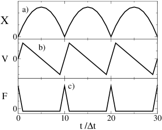
Figure 1: Schematic a) position, b) velocity, and c) force, in arbitrary units, for a particle moving in one dimension, generated by the mixed-force algorithm with zero initial velocity and a force correction interval of 10 time steps. For simplicity, the converged force is equal to zero and the cheap (fast) force is a negative constant. The periodic force correction ‘kicks’ are positive and invert the velocity. Notice that the position and velocity at the correction steps are equal to their correct converged value (zero).

For simplicity, we take the converged force and the initial velocity equal to zero, so that the correct converged position is also zero at all times. The mixed-force trajectory, for a constant negative fast force, shows periodic force kicks that change discontinuously the velocity and invert the trajectory at the correction steps.

We have applied this method to simulate a system of 64 silicon atoms at an average temperature of $\sim 2000$ K and an average pressure close to zero. This high temperature was intentionally chosen to test the method under specially stringent conditions, whith high kinetic energies and frequent formation and breaking of bonds. The simulations were performed with the SIESTA program Soler et al. (2002) but standard Hamiltonian diagonalizations were used instead of order-$N$ methods Ordejon et al. (1993); Kim et al. (1995), because of the metallic character of liquid silicon. For the cheap forces we use the Harris functional, a minimal basis set with a range of 3.5 and 4.0 Bohr for $s$ and $p$ orbitals, a real-space integration grid with a plane wave cutoff of 40 Ry, and only the $\Gamma$ $k$-point. For the converged forces, we use the self-consistent Kohn-Sham functional in the LDA, a double-$\zeta$ polarized (DZP) basis set with a range of 5.4, 6.5, and 3.8 for $s,p$ and $d$ basis orbitals, a real-space grid with a 80 Ry plane wave cutoff, and only the $\Gamma$ $k$-point. The forces are corrected according to equation (1) every $n$ time steps, with $\Delta t=1$ fs.

Figure 2 compares the magnitudes of the fast and converged forces, and of their difference.

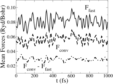
Figure 2: Decomposition of the total converged forces ${\bf F}_{conv}$ into a cheaply evaluated component ${\bf F}_{fast}$, and a remainder ${\bf F}_{conv}-{\bf F}_{fast}$. Represented are the average norms as a function of time. The trajectory was generated for 64 Si atoms at 2000 K, using the converged forces.

It can be seen that the latter is a relativelly small and smooth correction, what explains why it may be evaluated and applied less frequently.

Figure 3 represents the divergence of the trajectories, generated with different values of $n$, away from the reference converged trajectory (which corresponds to $n=1$ in Eq. (1)).

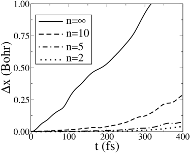
Figure 3: Divergence of the mixed-force MD trajectories from the converged-force trajectory for the liquid silicon system. $\Delta x$ is the average distance in atomic positions between the given and the reference trajectories. Force corrections were made every $n=2,5,10,20$, and $\infty$ (only fast forces) time steps.

It can be seen that even the $n=10$ trajectory diverges much more slowly than that obtained purely from the fast forces (labelled $n=\infty$, i.e. with no force corrections).

Figure 4 shows the total energy as a function of time.

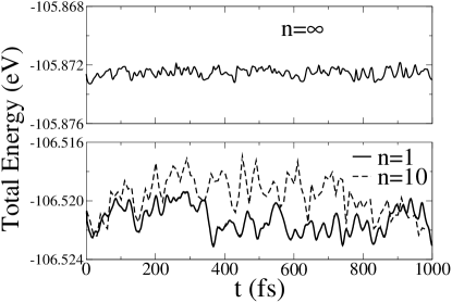
Figure 4: Total energy per atom, as a function of time, for the liquid silicon system. In the mixed-force ($n=10$) and converged-force ($n=1$) trajectories, the total energy was calculated at the correction steps, as the sum of the Kohn-Sham energy plus the nuclear repulsion and kinetic energies. In the fast-force trajectory ($n=\infty$), it was calculated at every step, using the Harris-functional for the electronic part. The standard deviations are 0.9, 1.3, and 0.3 meV/atom for the $n=1,10$, and $\infty$ trajectories, respectively.

The energy conservation is considerably worse in the selfconsistent converged-force trajectory ($n=1$) than in the Harris-force trajectory ($n=\infty$). This probably reflects larger effects of charge sloshings and analytic discontinuities in the forces, due to frequent level crossings in this highly disordered system. However, it is important to notice that the energy conservation in the mixed-force trajectory ($n=10$) is similar to that in the converged trajectory.

Despite the high simulation temperature, the charge transfer in elemental liquid silicon may be expected to be considerably smaller than in an ionic system, making the non-selfconsistent Harris functional specially adequate. In fact, we have seen that structural magnitudes like the bond length and bond angle distributions are not very different using the Kohn-Sham and Harris functionals. Therefore, we have also studied a more challenging system, liquid silica, using 72 atoms at a high average temperature of 5500 K and a low density of 0.42 g/cm³, typical of porous silica aerogels Rahmani et al. (2001). The distributions of bond legths and angles, presented in Figures 5 and 6, are indeed very different using the two functionals ($n=1$ and $n=\infty$).

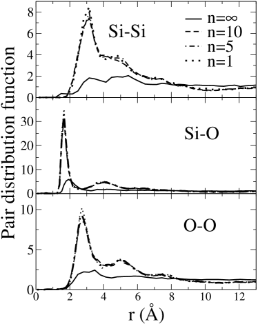
Figure 5: Radial pair distribution functions of liquid SiO₂ at 5500 K, using the new method with different values of $n$. The converged forces, used for $n=1$ and for the correction steps of $n=5$ and 10, were obtained with a double $\zeta$ plus polarization basis set, a real-space grid with a plane wave cutoff of 200 Ryd and only the $\Gamma$ $k$-point. The fast forces (that yield the $n=\infty$ curves when uncorrected) were calculated with a minimal basis set (single $\zeta$), a real-space grid with a plane wave cutoff of 150 Ryd and only the $\Gamma$ $k$-point.

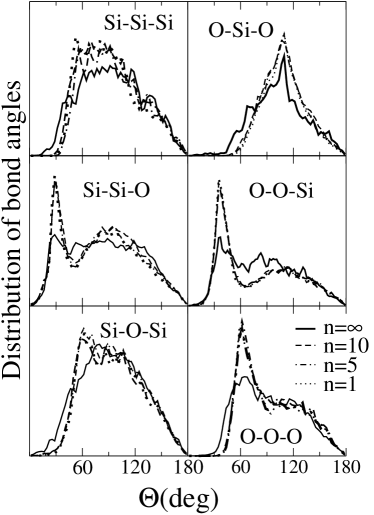
Figure 6: Bond-angle distribution functions of the liquid SiO₂ system, using the new method with different values of n. The bond cutoff radii were chosen 10% larger than the first maximum in the corresponding pair distribution functions of Fig. 5.

Despite this, the mixed-force method, with up to $n=10$, yields essentially the same distributions as the converged Kohn-Sham trajectory. Similar results, to be presented elsewhere, were obtained for an even more ionic system, liquid magnesium oxide, with 54 atoms at 6500 K and 30 GPa.

It might be expected that dynamical magnitudes are more sensitive than thermodynamic averages to changes in how the MD trajectories are obtained. Figure 7 shows the velocity autocorrelation function for the three systems studied, as a function of the interval $n$ between force corrections.

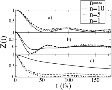
Figure 7: Velocity autocorrelation function $Z(t)=\langle{\bf v}_{i}(t^{\prime}){\bf v}_{i}(t^{\prime}+t)\rangle/\langle{\bf v}_{i}^{2}(t^{\prime})\rangle$, as a function of the interval $n$ between force corrections, for a) liquid Si at 2000 K and zero pressure, b) liquid MgO at 6500 K and 30 GPa, and c) liquid SiO₂ at 5500 K and a density of 0.42 g/cm³.

As expected, the trajectory of the non-selfconsistent Harris functional is reasonably accurate only for elemental liquid silicon. But, in every case, the mixed-force method, with up to $n=10$, yields essentially the same velocity autocorrelations as the converged Kohn-Sham trajectories. We have also calculated self-difussion coefficients from the average quadratic distances traversed as a funtion of time. Thus, for liquid silicon we obtain, respectively, $(2.4\pm 0.1)$, $(2.5\pm 0.1)$, $(2.6\pm 0.1)$, $(2.6\pm 0.1)$, and $(2.0\pm 0.1)\times 10^{-4}$ $\textrm{cm}^{2}/\textrm{s}$, for $n=1,5,10,20$ and $\infty$. Again, the mixed-force value, even with $n=20$, is the same, within the statistical error, as that of the converged trajectory. This indicates that dynamical and kinetic magnitudes, as well as structural or thermodynamic averages, are well reproduced even with quite large values of the boost factor $n$.

In conclusion, we have presented a new method to greatly accelerate ab initio molecular dynamics simulations by combining cheap force evaluations with accurate converged ones. Our results show that the method is very robust with respect to the reduced accuracy of the cheap forces. Although the acceleration factor will undoubtly depend on the system simulated, our present results indicate that factors of 10 can be expected in most cases.

We thank specially Gabriel Fabricius for discussions, for help with the liquid silicon parameterization, and for sharing with us his data-processing programs. We also acknowledge useful discussions with Emilio Artacho. This work has been supported by the Fundación Ramón Areces and by Spain’s MCyT grant BFM2000-1312.

References

- Allen and Tildesley (1987) M. P. Allen and D. J. Tildesley, Computer Simulation of Liquids (Oxford Univ. Press, Oxford, 1987).
- Bulatov et al. (1998) V. Bulatov, F. F. Abraham, L. Kubin, B. Devincre, and S. Yip, Nature 391, 669 (1998).
- Duan and Kollman (1998) Y. Duan and P. A. Kollman, Science 282, 740 (1998).
- Voter (1996) A. F. Voter, MRS Bull. 21, 17 (1996).
- Car and Parrinello (1985) R. Car and M. Parrinello, Phys. Rev. Lett. 55, 2471 (1985).
- Payne et al. (1992) M. C. Payne, M. P. Teter, D. C. Allan, T. A. Arias, and J. D. Joannopoulos, Rev. Mod. Phys. 64, 1045 (1992).
- Tuckerman et al. (1992) M. Tuckerman, B. J. Berne, and G. J. Martyna, J. Chem. Phys. 97, 1990 (1992).
- De Vita and Car (1998) A. De Vita and R. Car, Symp. Mater. Res. Soc. 491, 473 (1998).
- Ordejón et al. (1996) P. Ordejón, E. Artacho, and J. M. Soler, Phys. Rev. B 53, R10441 (1996).
- Soler et al. (2002) J. M. Soler, E. Artacho, J. D. Gale, A. García, J. Junquera, P. Ordejón, and D. Sánchez-Portal, J. Phys.: Condens. Matter 14, 2745 (2002).
- Kohn and Sham (1965) W. Kohn and L. J. Sham, Phys. Rev. 140, A1133 (1965).
- Troullier and Martins (1991) N. Troullier and J. L. Martins, Phys. Rev. B 43, 1993 (1991).
- Sankey and Niklewski (1989) O. F. Sankey and D. J. Niklewski, Phys. Rev. B 40, 3979 (1989).
- Anglada et al. (2002) E. Anglada, J. M. Soler, J. Junquera, and E. Artacho, Phys. Rev. B 66, 205101.1 (2002).
- Harris (1985) J. Harris, Phys. Rev. B 31, 1770 (1985).
- Batcho and Schlick (2001) P. F. Batcho and T. Schlick, J. Chem. Phys. 115, 4019 (2001).
- Ordejon et al. (1993) P. Ordejon, D. A. Drabold, M. P. Grumbach, and R. M. Martin, Phys. Rev. B 48, 14646 (1993).
- Kim et al. (1995) J. Kim, F. Mauri, and G. Galli, Phys. Rev. B 52, 1640 (1995).
- Rahmani et al. (2001) A. Rahmani, P. Jund, C. Benoit, and R. Julien, J. Phys.: Condens. Matter 13, 5413 (2001).