Spin splitting and precession in quantum dots with spin-orbit coupling: the role of spatial deformation

Abstract

Extending a previous work on spin precession in GaAs/AlGaAs quantum dots with spin-orbit coupling, we study the role of deformation in the external confinement. Small elliptical deformations are enough to alter the precessional characteristics at low magnetic fields. We obtain approximate expressions for the modified $g$ factor including weak Rashba and Dresselhaus spin-orbit terms. For more intense couplings numerical calculations are performed. We also study the influence of the magnetic field orientation on the spin splitting and the related anisotropy of the $g$ factor. Using realistic spin-orbit strengths our model calculations can reproduce the experimental spin-splittings reported by Hanson et al. (cond-mat/0303139) for a one-electron dot. For dots containing more electrons, Coulomb interaction effects are estimated within the local-spin-density approximation, showing that many features of the non-iteracting system are qualitatively preserved.

I Introduction

In the last years the study of spin-related phenomena has become one of the most active research branches in semiconductor physics. The present advances in spin-based electronicsWol01 and the hope for better devices, with enhanced performance with respect to the conventional charge-based ones, encourage this research. Two physical mechanisms underlie the operation of most spintronic devices: a) the spin-spin interaction, present in ferromagnetic materials and in diluted magnetic semiconductors; and b) the electron spin-orbit (SO) coupling stemming from relativistic corrections to the semiconductor Hamiltonian. It should also be mentioned that, as shown recently by Ciorga et al., another possibility of spin control involves the use of external magnetic fields to induce changes in the spin structure of a quantum dot.Cio03 These spin modifications affect the passage of currents through the system, originating the spin blockade effect. A conspicuous example of device exploiting the SO coupling is the spin transistor, first proposed by Datta and Das.Datxx In this system the spin rotation induced by an adjustable Rashba coupling is used to manipulate the current.

In a recent work,Valxx we studied the spin precession of quantum dots with SO coupling under the action of a vertical magnetic field of modulus $B$. It was shown that the SO coupling modifies the precessional frequency from the Larmor expression $\hbar\omega_{L}=|g^{*}|\mu_{B}B$, where $g^{*}$ is the bulk effective $g$ factor and $\mu_{B}$ is the Bohr magneton, to a different value depending on the dot quantum state. Namely, the modified precessional energy equals the gap between spin up and down states for the active level, the so called spin-flip gap $\Delta_{sf}$.

Purely circular dots are characterized by discontinuous jumps in angular momentum with the number of electrons $N$ and the magnetic field, with a similar behavior for the precessional frequency. An interesting prediction of Ref. Valxx, was that for some values of $N$ a finite $\Delta_{sf}$ persists even at $B=0$, i.e., a constant offset to the above Larmor formula. It is our aim in this work to extend those investigations by including deformation in the external confinement, as well as a more general treatment of the SO coupling, considering Rashba and Dresselhaus contributions on an equal footing. We shall show that small elliptical deformations are enough to sizeably alter the precessional frequency, yielding a deformation-dependent $g$ factor and washing out the low $B$ offsets of purely circular dots. Anisotropy effects in the $g$ factor will also be studied by allowing for a tilted orientation of the magnetic field vector with respect to the dot plane.

Spin dynamics in semiconductor nanostructures can be experimentally monitored with optical techniques. Indeed, a time-delayed laser interacting with a precessing spin experiences the Faraday rotation of its polarization. Measuring the rotation angle for different delays allows to map the spin orientation and thus observe in detail the dynamics. This technique has been applied to bulk semiconductors (see Ref. Kik99, for a recent review) and, also, to CdSe excitonic quantum dots in Ref. Gup99, . Alternative methods to gather information on the $g$ factor in quantum dots normally use measurements of the resonant tunneling currents through the system that permit the determination of the spin splittings and, therefore, deduce the effective $g$ value.Fuji02 ; Han03

Electron spin in quantum dots is much more stable than in bulk semiconductors, due to the suppression of spin flip decoherence mechanisms.Kha00 Spin relaxation is predicted to occur on a time scale of 1 ms for $B=1$ T. Accordingly, in this work we shall neglect spin relaxation, focussing on the much faster spin precession in quantum dots. The spin splittings will be compared with those measured in Ref. Han03, , showing that realistic values of the SO strengths can indeed reproduce the observed behavior. The paper is organized as follows. Section II presents the analytical model for low SO intensities. In Sec. III we discuss the numerical results for a variety of situations; namely, arbitrary SO strengths (A), tilted magnetic fields (B), one-electron dots (C) and treating Coulomb interaction effects (D) within the local-spin-density approximation (LSDA). Finally, the conclusions are presented in Sec. IV.

II The Model

II.1 The noninteracting Hamiltonian

Our model of a single quantum dot consists in $N$ electrons of effective mass $m^{*}$ whose motion is restricted to the $xy$ plane where an electrostatic potential $V_{\it ext}({\bf r})$ induces the confinement. We assume a GaAs host semiconductor, for which $m^{*}=0.067m_{e}$. To allow for elliptically deformed shapes we consider an anisotropic parabola, i.e.,

$$V_{\it ext}({\bf r})=\frac{1}{2}m^{*}(\omega_{x}^{2}x^{2}+\omega_{y}^{2}y^{2})\;.$$ (1)

Neglecting for the moment Coulomb interactions between electrons we treat the Hamiltonian for independent particles ${\cal H}_{ip}=\sum_{i=1}^{N}{h(i)}$. The single-electron Hamiltonian ($h$) contains the kinetic/confinement energy ($h_{0}$), the Rashba ($h_{R}$) and Dresselhaus ($h_{D}$) SO terms and the Zeeman energy ($h_{Z}$);

$$h=h_{0}+h_{R}+h_{D}+h_{Z}\;.$$ (2)

The explicit expressions of $h_{0}$ and $h_{Z}$ read

$$h_{0} = \frac{{\bf P}^{2}}{2m^{*}}+V_{\it ext}(x,y)\;,$$ (3)

$$h_{Z} = \frac{1}{2}g^{*}\mu_{B}(B_{x}\sigma_{x}+B_{y}\sigma_{y}+B_{z}\sigma_{z})\;;$$ (4)

where ${\bf P}=-i\hbar\nabla+\frac{e}{c}{\bf A}$ represents the canonical momentum depending on the vector potential ${\bf A}=B_{z}/2(-y,x)$ and the $\sigma$’s are the Pauli matrices (used also in the SO contributions). Note that all three components of the magnetic field contribute to the Zeeman term while only the vertical one couples with the kinetic energy through the vector potential. The GaAs bulk $g$ factor is $g^{*}=-0.44$. Finally, the Rashba and Dresselhaus SO Hamiltonians may be written asVosxx

$$h_{R} = \frac{\lambda_{R}}{\hbar}\left(\,P_{y}\sigma_{x}-P_{x}\sigma_{y}\,\right)\;,$$ (5)

$$h_{D} = \frac{\lambda_{D}}{\hbar}\left(\,P_{x}\sigma_{x}-P_{y}\sigma_{y}\,\right)\;.$$ (6)

The coupling constants $\lambda_{R}$ and $\lambda_{D}$ determine the SO strengths and their actual values may depend on the sample. Several experiments on quantum wells have recently provided valuable information about realistic ranges of variation for these coefficients.Nitxx

II.2 The analytical solution

It is possible to obtain analytical solutions when $h_{0}\gg(h_{R}\simeq h_{D})\gg h_{Z}$ and $B_{x}=B_{y}=0$. In this case one may use unitary transformations (as suggested in Ref. Ale01, ) yielding a diagonal transformed Hamiltonian. In a recent workValyy we used this technique to show that the SO (Dresselhaus) coupling induces oscillations between up and down spin states when the magnetic field or the dot deformation are varied. Generalizing the transformations to consider both SO terms we define

$$\tilde{h} = U_{1}^{\dagger}hU_{1}\;,$$

$$U_{1} = \exp\left\{\rule{0.0pt}{12.80365pt}-i\frac{m^{*}}{\hbar^{2}}\left[\rule{0.0pt}{9.95863pt}\lambda_{R}(y\sigma_{x}-x\sigma_{y})\right.\right.$$ (7)

$$\qquad\qquad\quad+\left.\rule{0.0pt}{12.80365pt}\left.\rule{0.0pt}{9.95863pt}\lambda_{D}(x\sigma_{x}-y\sigma_{y})\right]\right\}\;.$$

Expanding in powers of the $\lambda$’s one finds for the transformed Hamiltonian

$$\tilde{h} = {{\bf P}^{2}\over 2m^{*}}+V_{\it ext}(x,y)$$ (8)

$$- (\lambda_{R}^{2}-\lambda_{D}^{2})\frac{m^{*}}{\hbar^{3}}\,L_{z}\sigma_{z}+\frac{1}{2}\,g^{*}\mu_{B}B_{z}\sigma_{z}$$

$$- N(\lambda_{R}^{2}+\lambda_{D}^{2})\frac{m^{*}}{\hbar^{2}}+O(\lambda^{3})\;,$$

where we have defined the canonical angular momentum operator $L_{z}=xP_{y}-yP_{x}$. Note that to $O(\lambda^{2})$, with $\lambda$ referring to both $\lambda_{R}$ and $\lambda_{D}$, the Hamiltonian of Eq. (8) is diagonal in spin space. Nevertheless, the $x$ and $y$ spatial degrees of freedom are still coupled through the vector potential in the kinetic energy and in $L_{z}$.

A second transformation for each spin subspace of Eq. (8) may be used to obtain spatially decoupled oscillators. Namely, introducing a renormalized cyclotron frequency

$$\omega_{c\eta}={eB_{z}\over m^{*}c}+(\lambda_{D}^{2}-\lambda_{R}^{2})\,\frac{2m^{*}}{\hbar^{3}}\,s_{\eta}\;,$$ (9)

where $s_{\eta}=\pm 1$ for $\eta=\uparrow,\downarrow$, in Eqs. (5) of Ref. Valyy, one obtains the masses $M_{k\eta}$ and frequencies $\Omega_{k\eta}$ of the two ($k=1,2$) decoupled oscillators for each spin. Analogously, Eqs. (7) of that reference yields the eigenvalues $\varepsilon_{N_{1}N_{2}\eta}$, depending on the corresponding number of quanta in each oscillator ($N_{1},N_{2}$). For completeness of the presentation we repeat here the expressions for the latter two quantities,

$$\Omega_{k\eta} = \frac{1}{\sqrt{2}}\left(\rule{0.0pt}{14.22636pt}\right.\omega_{x}^{2}+\omega_{y}^{2}+\omega_{c\eta}^{2}$$ (10)

$$\pm \sqrt{\left(\omega_{x}^{2}+\omega_{y}^{2}+\omega_{c\eta}^{2}\right)^{2}-4\omega_{x}^{2}\omega_{y}^{2}}\left.\rule{0.0pt}{14.22636pt}\right)^{1/2}\;,$$

where the upper (lower) sign in $\pm$ corresponds to $k=1$(2), and

$$\varepsilon_{N_{1}N_{2}\eta} = \left(N_{1}+\frac{1}{2}\right)\hbar\Omega_{1\eta}+\left(N_{2}+\frac{1}{2}\right)\hbar\Omega_{2\eta}$$ (11)

$$+ s_{\eta}\frac{1}{2}g^{*}\mu_{B}B_{z}\;,$$

As a direct application of the above results we may write the effective $g$ factor for precession around a vertical magnetic field from the difference between the up and down single particle energies ($\Delta_{sf}$) with fixed oscillator quanta $N_{1}$ and $N_{2}$,

$$|g| \equiv \frac{\Delta_{sf}}{\mu_{B}B}$$ (12)

$$\!\!\!\!\!= \!\!\!\!\!\left|g^{*}+\frac{\hbar}{\mu_{B}B_{z}}\sum_{k=1,2}{\left(N_{k}+\frac{1}{2}\right)(\Omega_{k\uparrow}-\Omega_{k\downarrow})}\right|\;.$$

This equation shows that in the general case the $g$ factor is actually a function of the electron state (through the quanta), the SO coupling constants and the vertical magnetic field $B_{z}$ (through the $\Omega$’s). It is also worth to mention that since the energy gap $\Delta_{sf}$ and the modulus of the magnetic field ($B$) are positive quantities, only the absolute value of the $g$ factor is determined by Eq. (12).

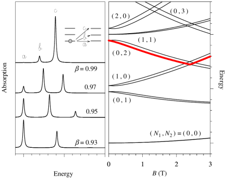
Figure 1: Right panel: Evolution of the single particle energies as a function of vertical magnetic field. Each doublet corresponds to different spin orientations in the transformed frame (Sec. II.B). The SO intensity is fixed at $\lambda_{D}^{2}-\lambda_{R}^{2}=(1.2\times 10^{-9}\,{\rm eV}\,{\rm cm})^{2}$. The level responsible for the spin-flip transition when $N=7$ is marked with a thick line. Left panel: Strength of the spin-flip excitation for different deformations ($\omega_{x}=\beta\omega_{y}$; $\hbar(\omega_{x}+\omega_{y})=12$ meV). The inset characterizes the transitions for $N=7$ and $B=0$ of the right panel, with $a$ indicating the transition between Kramers conjugates.

II.3 The transition between Kramers conjugates

When ${\bf B}$ vanishes the full Hamiltonian fulfills time-reversal symmetry and, according to a well known theorem of quantum mechanics, in that limit a degeneracy should prevail (Kramers degeneracy). As shown in Fig. 1, the single-particle energies $\varepsilon_{N_{1}N_{2}\eta}$ indeed merge into degenerate pairs at vanishing magnetic field. These pairs are split by the combined action of the SO and magnetic field contributions and for a given $(N_{1},N_{2})$ one obtains parallel doublets when increasing $B$. Depending on the sign of $\lambda_{D}^{2}-\lambda_{R}^{2}$ the lower member of each doublet will have a given spin orientation in the transformed frame; namely, upwards for positive sign and downwards for negative sign.

If the system has good angular momentum in the intrinsec reference frame ($L_{z}$), as happens in a circular confinement $\omega_{x}=\omega_{y}$, the Kramers conjugates at $B=0$ possess opposite angular momenta. Therefore, the spin flip transition between them is forbidden since the relevant matrix element preserves angular momentum. On the contrary, when the system is deformed, for instance due to an anisotropic confinement $\omega_{x}=\beta\omega_{y}$, the spin flip transition between Kramers conjugates becomes possible since angular momentum is no longer a ’good’ quantum number. This key point determines qualitatively different spin precessional spectra. In fact, when the transition between conjugates is forbidden there is a gap in the spectrum and a non-vanishing precession frequency at $B=0$ (the precessional offset discussed in Ref. Valyy, ). This gap vanishes if the transition between conjugates is allowed due to the deformation. In the left panel of Fig. 1 we show the evolution of the precessional peaks as the deformation is reduced ($\beta\to 1$). As discussed, the transition between Kramers conjugates ($a$) switches off when approaching the circular case.

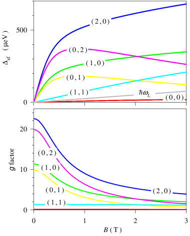
Figure 2: Upper: spin-flip energy gap for the different levels of Fig. 1. The Larmor energy $\hbar\omega_{L}$ is also indicated. Lower: g factors in absolute value inferred from the upper panel results as $|g|=\Delta_{sf}/(\mu_{B}B)$.

II.4 The $g$ factors

The upper panel of Fig. 2 displays the spin-flip gap for different levels, characterized by their oscillator quanta in the transformed frame. The lower panel shows the corresponding $g$ factors obtained from $\Delta_{sf}$ and the modulus of the magnetic field using the first equality of Eq. (12). As in Fig. 1 a SO value of $\lambda_{D}^{2}-\lambda_{R}^{2}=(1.2\times 10^{-9}\,{\rm eV}\,{\rm cm})^{2}$ as well as a deformation of $\beta=0.9$ have been assumed. We note that there is a strong dependence of the precessional properties on the electronic state, with many cases showing a dramatic deviation from the Larmor result. When the number of quanta is shared asymmetrically between the two oscillators the $g$ factor takes very large values at small magnetic fields, decreasing quite abruptly with $B$. On the contrary, when $N_{1}=N_{2}$ there is a rather flat $B$-dependence of the $g$ factor and lower enhancements. Note also that spin-flip energies below the Larmor result are obtained for the $(0,0)$ state, implying a $g$ factor lower than the bare value. We have checked that other values of the SO couplings and dot deformations do not lead to qualitative variations of this behaviors although, obviously, the numerical values are changed.

III Cases of numerical treatment

When the SO coupling can not be considered weak or when the magnetic field points in a tilted orientation, with respect to the $z$ axis, the above analytical treatment does not remain valid. One must then resort to direct numerical solution of the single-particle Schrödinger equation

$$h\,\varphi_{i}({\bf r},\eta)=\varepsilon_{i}\,\varphi_{i}({\bf r},\eta)\;.$$ (13)

As in Ref. Valyy, , we have proceeded by discretizing in a uniform grid of points, finding the orbitals and energies $\{\varphi_{i}({\bf r},\eta),\varepsilon_{i}\}$ using matrix techniques. In terms of these results one can directly compute the spin-flip strength function,

$$S_{\it prec}(\omega) = \sum_{ij}{(1-f_{i})f_{j}\,\left|\langle\varphi_{i}|\sigma_{x}|\varphi_{j}\rangle\right|^{2}}$$ (14)

$$\times \delta(\varepsilon_{i}-\varepsilon_{j}-\hbar\omega)\;,$$

where $i$ and $j$ span the whole single particle set and the $f_{i}$’s give the orbital occupations.

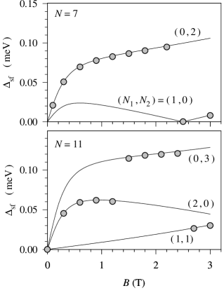
Figure 3: Numerical results for the spin-flip gap when $\lambda_{R}=0$ and $\lambda_{D}=0.5\times 10^{-9}$ eVcm. For comparison the solid line display the analytical results from Eq. (12).

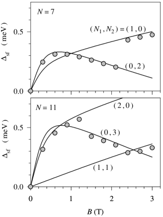
Figure 4: Same as Fig. 3 but for $\lambda_{R}=1.2\times 10^{-9}$ eVcm and $\lambda_{D}=0$.

III.1 Vertical magnetic fields

We have checked that the numerical solution recovers the previously discussed analytical limit for vertical magnetic fields and weak SO couplings. For instance, Fig. 3 compares the spin-flip gaps for cases with a weak pure Dresselhaus coupling having $N=7$ and 11 electrons. An excellent agreement between the numerical data and the prediction of Eq. (11) is found. Note that in the numerical case discontinuous jumps in the evolution of $\Delta_{sf}$ as a function of $B$ are obtained whenever the ground-state solution implies a reordering of levels in energy. Figure 4 displays a similar result for a pure Rashba coupling, with a somewhat stronger intensity. Small deviations can be seen with the analytical result, although the agreement is still quite good. Our results thus indicate that the analytic treatment works rather well for SO couplings as large as $1.2\times 10^{-9}$ eV cm, which is in the range of the experimentally achieved values.

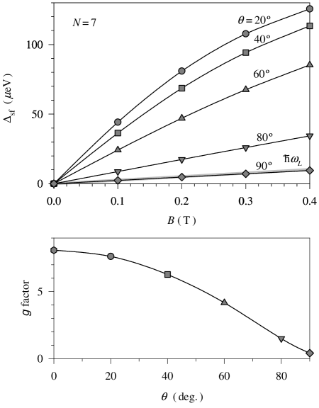
Figure 5: Upper: Dependence of the spin-flip gap on the tilting angle of the magnetic field with respect to the vertical direction. The thick gray line shows the Larmor energy. Lower: Variation of the g factors in the limit $B\to 0$ as a function of the tilting angle $\theta$.

III.2 Tilted magnetic fields

In Fig. 5 we have analyzed the dependence of the precessional properties on the tilting angle of the magnetic field with respect to the $z$ axis, zero angle meaning perpendicular magnetic field and $\theta=90^{\rm o}$ parallel ${\bf B}$ to the plane of motion. Note that the spin-orbit interaction is not invariant under rotations in the $x-y$ plane so that its effects depend on the particular direction of tilting. In practice, however, different directions lead to only subtle differences, whilst the strong dependence is given by the angle $\theta$. For this reason we only discuss the case of tilting along the $x$-axis. We find a rather strong dependence of the spin-flip gap on the tilting angle, with a maximum deviation from the Larmor energy for perpendicular field. When the tilting angle is increased a smooth energy decrease in the direction of the Larmor value is seen. Actually, for parallel orientation the results are slightly below the Larmor line. In the lower panel of Fig. 5 the $g$ factors in the limit of vanishing magnetic field are displayed. In correspondence with the transition energies the largest deviations from the bulk value are obtained for the perpendicular direction while the parallel $g$ factor is more similar to the bare factor (0.44). These results can be understood by noting that the SO mechanism couples better with the ${\bf B}$-induced currents in the perpendicular geometry and, therefore, a larger influence on the spin precession is expected in this case.

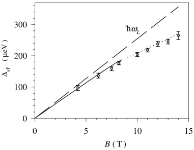
Figure 6: Experimental spin-flip energy gaps measured in Ref. Han03, for a one-electron dot. The solid line is the theoretical result obtained using the experimentally known $\omega_{0}$ values while the dotted extension is a fit (see Sec. III.C).

III.3 A comparison with experiment

In a recent experiment Hanson et al.Han03 have measured the spin splitting in a one-electron dot by means of conductivity experiments using a parallel magnetic field. It is our purpose here to show that the SO-induced modifications can be the source of the observed deviation of the spin-flip energy with respect to the Larmor result. As stated in the previous section, when the magnetic field is alligned parallel to the plane of electronic motion the spin splitting recovers a Zeeman-like behavior with an effective $g$-factor slightly smaller than the bulk value. This reduction of the spin splitting is enhanced as the spacing of the orbital levels is reduced, i.e., spin-orbit interaction induces a compression of the spin levels as $\omega_{x}$ and $\omega_{y}$ become smaller.

In Fig. 6 we display the results obtained for a circular 1-electron dot (deformation has no significant influence on the spin-splitting of the lowest energy state) with feasible values of SO coupling. Namely, we assumed $\lambda_{R}=0.35\times 10^{-9}$ eVcm, in the range of experimental values for GaAs,Vag98 and $\lambda_{D}=0.8\times 10^{-9}$ eVcm. This latter parameter is obtained by assuming a 2DEG width $z_{0}\simeq 60$ Å in the formula $\lambda_{D}=\gamma(\pi/z_{0})^{2}$, where $\gamma=27.5$ eVų is the GaAs specific constant.Vosxx We still need to input the external confinement frequency $\hbar\omega_{0}$ before the calculation can be performed. Using for this parameter the measured values of the orbital level spacing, lying between 0.96 and 1.1 meV for the range from $B=0$ to 8 T,priv one obtains the solid line of Fig. 6. For higher values of the magnetic field experimental values are not available and we have inferred the $\hbar\omega_{0}$ values in order to fit the measured spin splittings. By assuming $\hbar\omega_{0}\approx 0.5-0.6$ meV we obtain the dashed line in Fig. 6. Overall, the agreement with the measurements is rather good and, though this is a certainly a simplified model, we believe it indicates that SO coupling plays an important role in explaining the measured spin gaps in this system.

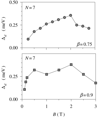
Figure 7: Spin precessional energies within TDLSDA. The magnetic field points in the vertical ($z$) direction.

III.4 Addition of Coulomb interactions

The above sections have dealt with the SO-induced modifications of the spin precession in the absence of Coulomb interaction between electrons. We shall now estimate the role of the latter by resorting to the time-dependent local-spin-density approximation (TDLSDA) for noncollinear spins. This approach was already used by us in Ref. Valyy, for circular dots. The reader is addressed to that reference for more details on this formalism. Here we shall only mention that the integration in time of the TDLSDA equations allows us to monitor the spin precession and, in particular, to extract the precessional frequencies. Since the selfconsistent parts of the mean-field potential are recomputed as the system evolves in time one is effectively taking into account dynamical interaction effects. The formalism is thus equivalent to the random-phase approximation (well known in many body theory) with an effective interaction.

Figure 7 shows for some representative cases the precessional frequencies in TDLSDA with SO coupling and deformation. A vertical magnetic field has been also included. We note that a qualitatively similar behaviour is found with respect to the preceding analytical results. In particular, we emphasize that at small $B$ the precessional frequency tends to vanish and that there are discontinuous jumps due to level rearrangements. It can be seen that, for a higher deformation (smaller $\beta$), the $B$-dependence of the precessional frequencies is smoother, in agreement with the analytical model. Comparing with the non-interacting results there is a sizeable modification of the evolution in the low $B$ range. While in the non-interacting scheme we obtain $g$ factors of 20 and 6.2 for $\beta=0.9$ and 0.75, respectively, when interaction is included these values raise to 21.9 and 6.55.

IV Conclusions

In this work we have analyzed the role of the deformation in the confinement to determine, in conjunction with SO coupling and magnetic field, the spin precessional properties of GaAs quantum dots. At small magnetic fields the deformation closes the spin-flip energy gap by allowing the transition between Kramers conjugate states. In practice, this implies that the precessional frequencies of deformed systems have no offsets at $B=0$. The associated $g$ factors depend strongly on the quantum dot electronic state and on the magnetic field direction. By tilting ${\bf B}$ from vertical to horizontal direction one may tune the $g$ factor from large values to results close to the bulk one.

When the magnetic field points in the vertical direction and the SO coupling is weak an analytical treatment, yielding the spin-flip energies and $g$ factors is possible. This provides relevant insights for the analysis of other cases that can only be addressed with numerical approaches. For the case of a one-electron dot in a horizontal magnetic field we have compared the results obtained with feasible values of the SO coupling constants with recent experiments. We believe this comparison indicates that the SO coupling plays an important role in explaining the measured spin gaps in this system. For dots containing more electrons, the role of the Coulomb interactions has been estimated within TDLSDA. Sizeable modifications of the single-particle picture have been obtained although, qualitatively, the main features are preserved.

- (1) S. A. Wolf, D. D. Awschalom, R. A. Buhrman, J. M. Daughton, S. von Molnár, M. L. Roukes, A. Y. Chtchelkanova, D. M. Treger, Science 294, 1488 (2001).
- (2) M. Ciorga, A. S. Sachrajda, P. Hawrylak, C. Gould, P. Zawadzki, S. Jullian, Y. Feng, and Z. Wasilewski, Phys. Rev. B 61, R16315 (2000).
- (3) S. Datta and B. Das, Appl. Phys. Lett. 56, 665 (1990).
- (4) M. Valín-Rodríguez, A. Puente, Ll. Serra, and E. Lipparini, Phys. Rev. B 66, 235322 (2002).
- (5) D.D. Awschalom and J. M. Kikkawa, Physics Today 52, 33 (1999).
- (6) J. A. Gupta, D. D. Awschalom, X. Peng, A. P. Alivisatos, Phys. Rev. B 59, 10421 (1999); J. A. Gupta, D. D. Awschalom, Al. L. Efros, A.V. Rodina, Phys. Rev. B 66, 125307 (2002).
- (7) T. Fujisawa, D. G. Austing, Y. Tokura, Y. Hirayama, S. Tarucha, Nature 419, 278 (2002).
- (8) R. Hanson, B. Witkamp, L. M. K. Vandersypen, L.H. Willems van Beveren, J. M. Elzerman, and L.P. Kouwenhoven, preprint (cond-mat/0303139).
- (9) A. V. Khaetskii, Y. V. Nazarov, Phys. Rev. B 64, 125316 (2001).
- (10) O. Voskoboynikov, C. P. Lee, O. Tretyak, Phys. Rev. B 63, 165306 (2001).
- (11) T. Koga, J. Nitta, H. Takayanagi, S. Datta, Phys. Rev. Lett. 88, 126601 (2002).
- (12) I. L. Aleiner and V. I. Fal’ko, Phys. Rev. Lett. 87, 256801 (2001).
- (13) M. Valín-Rodríguez, A. Puente, Ll. Serra, and E. Lipparini, Phys. Rev. B 66, 165302 (2002).
- (14) H. D. Meyer, J. Kucar, and L. S. Cederbaum, J. Math. Phys. (N.Y.) 29, 1417 (1988).
- (15) I.D. Vagner, A.S. Rozhavsky, P. Wyder, A. Yu. Zyuzin. Phys. Rev. Lett. 80, 2417 (1998).
- (16) Private communication.