Biologically inspired learning in a layered neural net

Abstract

A feed–forward neural net with adaptable synaptic weights and fixed, zero or non–zero threshold potentials is studied, in the presence of a global feedback signal that can only have two values, depending on whether the output of the network in reaction to its input is right or wrong.

It is found, on the basis of four biologically motivated assumptions, that only two forms of learning are possible, Hebbian and Anti–Hebbian learning. Hebbian learning should take place when the output is right, while there should be Anti–Hebbian learning when the output is wrong.

For the Anti–Hebbian part of the learning rule a particular choice is made, which guarantees an adequate average neuronal activity without the need of introducing, by hand, control mechanisms like extremal dynamics. A network with realistic, i.e., non–zero threshold potentials is shown to perform its task of realizing the desired input–output relations best if it is sufficiently diluted, i.e. if only a relatively low fraction of all possible synaptic connections is realized.

I Introduction

In this article we will try to contribute to the study of biological neural networks, in particular with respect to learning. Since we are interested in the basic principles rather than subtle biological details, we will use simplified models, although we do not allow for any properties that are unrealistic from a biological point of view. In this way we hope to reveal the essentials, without blurring the analysis with (irrelevant, biological) details.

It is also not our aim to construct a network that is optimized for some particular task; our only purpose is to study a model that resembles an actual biological neural net and the way it might learn.

In section II we define the model that we will study: a simple feed–forward network with one hidden layer of which not all possible connections are present (i.e., dilution unequal zero). Each neuron of the net has three variables associated with it: a (fixed) threshold potential $\theta$, a (variable) membrane potential $h$ and a state $x$, which is assumed to take two values only, depending on the fact whether the neuron fires or is quiescent.

This article fits into a line of biologically motivated research. Chialvo and Bak bak suggested learning by punishment only, via the release of some hormone. Heerema et al. leeuwen derived rules for a biological neural net when it acts as a memory. Bosman et al. bosman added this rule to the model of Chialvo and Bak, and, thereby, found a significant improvement of the network’s performance.

The dynamics of a neural net is determined by a rule that tells a neuron when to fire. A biological neuron fires if its membrane potential $h$ exceeds its threshold $\theta$. In the model of Chialvo and Bak this biological rule is replaced by the rule that in each layer a fixed number of neurons, having the highest membrane potentials, fire. They refer to this rule by the name of ‘extremal dynamics’. Extremal dynamics has the drawback that the number of active neurons is artificially fixed, restricting the number of possible output states. Alstrøm and Stassinopoulos alstrom did not use extremal dynamics, but they ran into the difficulty that the network’s activity became too small or too large for the network to function satisfactorily. In order to keep the activity at a desired level, they adapted the neuron threshold potentials $\theta$ at each step of the learning process.

It is one of our purposes to find a way in which a biological net can keep its neuronal activity around an acceptable level. Instead of putting in, by hand, some controlling mechanism, we started from four biologically motivated assumptions (III.1), which lead to the conclusion that only the so–called Hebbian and Anti–Hebbian learning rules are the plausible ones. We show that the Hebbian learning rule fixes and strengthens the action of the network at the moment it is applied, while the Anti–Hebbian learning rule does the opposite, and, when applied repeatedly, will change the network’s action. We conclude that Hebbian learning should be associated with reward, and should be applied if the network realizes the desired output state in reaction to its input, while Anti–Hebbian learning should be associated with punishment, and should be applied when the output of the network is wrong, in order to enable the network to search for better output (III.2).

In section III.3 we propose a particularly simple Anti–Hebbian learning rule (essentially two constants) of which we expect, however, that it will keep the activity of the neural network around a desired value automatically, i.e., without the need of some controlling mechanism. In section V, we perform a number of numerical simulations, the details of which are given in section IV, in order to verify whether our rule is capable of keeping the activity around a desired level. Because the Hebbian learning rule is already studied in leeuwen , we will first focus, in section V, on the effect of the Anti–Hebbian learning rule. Our simulations show that our Anti–Hebbian learning rule indeed is successful in keeping the average activity around a desired level, and, moreover, is very efficient in generating different output states with adequate activities.

Having studied the effect of the Anti–Hebbian learning rule we simulate, in section VI, networks using the complete learning rule, including both the Hebbian and the Anti–Hebbian contributions. We show that the complete learning rule enables the network to learn a number of input–output relations with an acceptable efficiency. Furthermore, it is shown that for non–zero threshold potentials, the performance is only acceptable if the network is sufficiently diluted. So ‘cutting away’ synaptic connections enhances the performance of the network. The observation that – in our model – some degree of non–connectedness is a conditio sine qua non for a properly functioning biological net, is one of our main observations.

The article closes with conclusions (section VII) and an outlook (section VIII).

II Modeling learning

In this section we describe our model and define quantities like activity and performance.

II.1 Network model

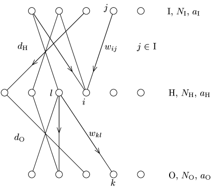
Figure 1: The feed–forward network has one hidden layer. The symbols I, H and O refer to the Input, Hidden and Output layers. In order to denote that a neuron $i$ of the net belongs to one of these layers we will write $i\in\text{I}$, $i\in\text{H}$ or $i\in\text{O}$, respectively. Furthermore, $N_{\text{X}}$ denotes the number of neurons in layer X (X = I, H or O). The weights of the synapses connecting either the input layer with the hidden layer or the hidden layer with the output layer both are indicated by the symbol $w_{ij}$. In this feed–forward network there are maximally $N_{\text{I}}N_{\text{H}}$ possible connections from the input layer to the hidden layer. If only the fraction $(1-d_{\text{H}})$, $0\leq d_{\text{H}}\leq 1$, of these connections to the hidden layer is actually realized, we call $d_{\text{H}}$ the dilution (of the connections with H). Similarly, $d_{\text{O}}$ is the dilution of the connections from the hidden layer to the output layer.

We consider a feed–forward neural net with one hidden layer (figure 1). The net is taken to be diluted, i.e. not all neurons are connected to all others. There are connections from the input layer to the hidden layer and from the hidden layer to the output layer but there are no direct connections from the input layer to the output layer nor any lateral or feed–back connections.

Let us suppose that the neural net consists of $N$ binary neurons $i$, $i=1,2,\ldots,N$. We will use the symbols I, H and O to refer to the Input, Hidden and Output layers. In order to denote that a neuron $i$ of the net belongs to one of these layers we will write $i\in\text{I}$, $i\in\text{H}$ or $i\in\text{O}$, respectively. The state $x_{i}$ of neuron $i$ either is active ($x_{i}=1$) or is non–active ($x_{i}=0$). The potential $h_{i}$, the difference in potential between the inner and the outer part of a neuron, is supposed to depend linearly on the activities of the incoming synaptic connections:

$$h_{i}=\sum_{j\in V_{i}}w_{ij}x_{j}$$ (1)

where $V_{i}$ is the collection of neurons $j$ that have an afferent synaptic connection to neuron $i$. This formula can be viewed as the defining expression for the weights $w_{ij}$. Since the $x_{i}$’s are chosen to be dimensionless, the weights have the dimension of a potential. Let $\theta_{i}$ be the potential that should be exceeded in order that neuron $i$ becomes active, i.e.,

$$x_{i}=1\quad\text{if}\quad h_{i}>\theta_{i},\quad x_{i}=0\quad\text{if}\quad h_{i}<\theta_{i}.$$ (2)

An alternative way to specify the state of neuron $i$ as given by equation (2), is to write

$$x_{i}=\Theta_{\text{H}}(h_{i}-\theta_{i}).$$ (3)

The function $\Theta_{\text{H}}$ is the Heaviside step–function [$\Theta_{\text{H}}(y)=0$ if $y<0$ and $\Theta_{\text{H}}(y)=1$ if $y>0$]. The state of the neurons of the input layer determine the state of the hidden layer via (1) and (3). The state of the hidden layer, in turn, determines the state of the output layer. Thus, if the states $x_{i}$ for $i\in\text{I}$ are given at each time step $t_{n}$, we can determine the network state at every time $t_{n}$, once we have a rule that fixes the $w_{ij}$ at time $t_{n}$ ($n=0,1,2,\ldots$).

The number of neurons in layer X (X = I, H or O) is denoted by $N_{\text{X}}$. The activity $a_{\text{X}}$ in layer X is defined by

$$a_{\text{X}}=\frac{1}{N_{\text{X}}}\sum_{i\in\text{X}}x_{i},\quad\text{X}=\text{I},\text{H},\text{O}.$$ (4)

The weights of the synapses connecting either the input layer with the hidden layer or the hidden layer with the output layer both are indicated by the symbol $w_{ij}$.

In this feed–forward network there are maximally $N_{\text{I}}N_{\text{H}}$ possible connections from the input layer to the hidden layer. If only the fraction $(1-d_{\text{H}})$, $0\leq d_{\text{H}}\leq 1$, of these connections to the hidden layer is actually realized, we call $d_{\text{H}}$ the dilution (of the connections with H). Similarly, $d_{\text{O}}$ is the dilution of the connections from the hidden layer to the output layer.

II.2 Learning input–output relations

Let us denote the state of layer X by $\bm{x}_{\text{X}}=(x_{\text{X}1},x_{\text{X}2},\ldots,x_{\text{X}N_{\text{X}}})$. We want the network to associate with a particular, prescribed input state $\bm{\xi}^{\mu}_{\text{I}}$, chosen from a collection of $p$ input states $\bm{\xi}^{\mu}_{\text{I}}$ ($\mu=1,\ldots,p$), the particular state $\bm{\xi}^{\mu}_{\text{O}}$, chosen from a collection of $p$ prescribed output states $\bm{\xi}^{\mu}_{\text{O}}$ ($\mu=1,\ldots,p$). The goal of the learning process is that the network will be able to generate, for all input patterns $\bm{\xi}^{\mu}_{\text{I}}$, the correct output pattern $\bm{\xi}^{\mu}_{\text{O}}$. This will be achieved by a learning procedure, in which the weights are adapted, stepwise, according to some rule.

If we present a pattern $\bm{\xi}^{\mu}_{\text{I}}$ to the network by setting $\bm{x}_{\text{I}}$ equal to $\bm{\xi}^{\mu}_{\text{I}}$, the network will respond by generating an output state $\bm{x}_{\text{O}}$ which, in general, will not be equal to the desired output state $\bm{\xi}^{\mu}_{\text{O}}$. We will associate a variable $r$ with each of the following two possibilities: $r=1$ if the output is right, i.e., if $\bm{x}_{\text{O}}=\bm{\xi}^{\mu}_{\text{O}}$ and $r=0$ if the output is wrong, i.e., if $\bm{x}_{\text{O}}\neq\bm{\xi}^{\mu}_{\text{O}}$. In practice, we proceed as follows. We present the first input pattern $\bm{\xi}^{1}_{\text{I}}$ to the net, which results in an output state $\bm{x}_{\text{O}}$. We keep repeating this until $\bm{x}_{\text{O}}$ equals $\bm{\xi}^{1}_{\text{O}}$, the output pattern to be associated with the input pattern $\bm{\xi}^{1}_{\text{I}}$. The net then has ‘learned’ the first input–output relation $(\bm{\xi}^{1}_{\text{I}},\bm{\xi}^{1}_{\text{O}})$. Next, we present the second input pattern, and continue until the second input–output relation $(\bm{\xi}^{2}_{\text{I}},\bm{\xi}^{2}_{\text{O}})$ has been learned, and so on until the $p$–th input–output relation $(\bm{\xi}^{p}_{\text{I}},\bm{\xi}^{p}_{\text{O}})$ has been learned. While doing so, we continuously change the weights according to some $r$–dependent rule: the ‘learning rule’.

When an input–output relation has been learned, one or more input–output relations learned earlier may have been forgotten. Therefore, we start a second round, in which we try to learn all $p$ input–output relations $(\bm{\xi}^{\mu}_{\text{I}},\bm{\xi}^{\mu}_{\text{O}})$ again. In order to prevent possible effects due to a specific learning order, the patterns are presented to the network in random order: each round their order is shuffled. After a number of rounds all input–output relations should be recalled at once, i.e., input $\bm{\xi}^{\mu}_{\text{I}}$ should result immediately in output $\bm{\xi}^{\mu}_{\text{O}}$ for all input–output relations.

Do learning rules exist which accomplish all this? The answer is positive bak ; bosman . A particular useful one is the one proposed in section III.

II.3 Performance

In order to judge the performance of our network, we need some measure.

The a priori probability $P(N_{\text{O}}^{(a)})$ that the state of the output layer $\bm{x}_{\text{O}}$ equals $(1,1,\ldots,1,0,0,\ldots,0)$, i.e., the state with the first $N_{\text{O}}^{(a)}$ elements equal to one and the remaining last $N_{\text{O}}-N_{\text{O}}^{(a)}$ elements equal to zero, is given by

$$P(N_{\text{O}}^{(a)})=p_{\text{O}}^{N^{(a)}_{\text{O}}}(1-p_{\text{O}})^{N_{\text{O}}-N^{(a)}_{\text{O}}}$$ (5)

where $p_{\text{O}}$ is the probability that an arbitrary neuron of the output layer is active ($0\leq p_{\text{O}}\leq 1$). Note that the probability to find an output pattern with $N_{\text{O}}^{(a)}$ active neurons at arbitrary places is also given by (5). Let $N^{(a)}_{\text{O}}(\bm{\xi}^{\mu}_{\text{O}})$ be the number of active neurons in pattern $\bm{\xi}^{\mu}_{\text{O}}$. Then, the average a priori number of trials needed to arrive at the desired output pattern equals $1/P(N^{(a)}_{\text{O}}(\bm{\xi}^{\mu}_{\text{O}}))$. If $p$ input–output relations $(\bm{\xi}^{\mu}_{\text{I}},\bm{\xi}^{\mu}_{\text{O}})$ are to be realized, ($\mu=1,\ldots,p$), the average a priori number $M_{a}$ of trials needed equals

$$M_{a}=\sum_{\mu=1}^{p}1/P(N^{(a)}_{\text{O}}(\bm{\xi}^{\mu}_{\text{O}})).$$ (6)

Comparing the average a priori number of trials and the actual average number of trials $M$ needed to learn all $p$ input–output relations we get a measure of how well the network performs. This leads us to define the performance $R$ as the quotient

$$R:=M_{a}/M$$ (7)

with $M_{a}$ given by (6). Note that the performance tends to zero when the network is unable to learn all input–output relations ($M\rightarrow\infty$) and the performance will be 1 for an ‘ideal’ network ($M=M_{a}$).

In some models bak ; bosman , the number of neurons that fire is fixed in some way. The a priori probability $P_{\text{fixed}}(N_{\text{O}}^{(a)}(\bm{\xi}^{\mu}_{\text{O}}))$ that the output state $\bm{x}_{\text{O}}$ equals the output pattern $\bm{\xi}^{\mu}_{\text{O}}$ is then given by

$$P_{\text{fixed}}(N_{\text{O}}^{(a)}(\bm{\xi}^{\mu}_{\text{O}}))=\frac{N_{\text{O}}^{(a)}(\bm{\xi}^{\mu}_{\text{O}})!(N_{\text{O}}-N_{\text{O}}^{(a)}(\bm{\xi}^{\mu}_{\text{O}}))!}{N_{\text{O}}!},$$ (8)

the inverse of the number of ways that a state with $N_{\text{O}}^{(a)}$ active neurons can be realized.

II.4 Activity distribution

Let us consider an arbitrary collection of $M$ neurons, all of which have (independent) probabilities $p$ to fire ($0\leq p\leq 1$). Then the probability $Q(a)$ that the activity of this collection of $M$ neurons equals $a$ is given by

$$Q(a)=\frac{M!}{(Ma)![M(1-a)]!}p^{Ma}(1-p)^{M(1-a)},$$ (9)

where $Ma$ is the number of neurons that fire ($Ma$ is an integer). This formula differs from (5) by a binomial factor, corresponding to the fact that there are $M!/\{(Ma)![M(1-a)]!\}$ possible states with the same activity $a$. We will use this formula in section V when we compare $Q(a)$ to the actual activity of the net.

II.5 Stability coefficient

Let us define the ‘two time stability coefficient’

$$\gamma_{i}(t_{n},t_{m}):=\left(2x_{i}(t_{n})-1\right)\left(h_{i}(t_{m})-\theta_{i}\right)$$ (10)

which is a generalization of the usual stability coefficient kinzel . With equation (3) it follows that, at two times $t_{n}$ and $t_{m}$ we have

$$\gamma_{i}(t_{n},t_{m})>0\Longrightarrow x_{i}(t_{n})=x_{i}(t_{m})$$ (11)

$$\gamma_{i}(t_{n},t_{m})<0\Longrightarrow x_{i}(t_{n})\neq x_{i}(t_{m}).$$ (12)

In particular, if $n=m$, we have

$$\gamma_{i}(t_{n},t_{n})>0.$$ (13)

The state of neuron $i$ does not change if $\gamma_{i}(t_{n},t_{m})$ is positive. Moreover, the larger $\gamma_{i}(t_{n},t_{n})$, the more stable the system is with respect to changes in the synaptic weights krauth ; gardner . The $\gamma$’s will play a role in section III.2.

III Determining the learning rule

As noted in the introduction, many neural networks have a tendency to develop into a state where most neurons are either all active or non–active. Chialvo and Bak bak and Alstrøm and Stassinopoulos alstrom solved this problem in a biologically less plausible way: the authors do not consider the threshold potentials at all bak , or allow them to grow indefinitely alstrom . We approach the problem in a different way: we start from four biologically plausible restrictions on the learning rule. This leads to the conclusion that the learning rule can be seen as a superposition of two types of learning, Hebbian and Anti–Hebbian learning. Taking for the Anti–Hebbian part the most simple ansatz one can think of in dependence of the state $x_{i}$ of the postsynaptic neuron $i$, we arrive at a learning rule that, a priori, is biologically plausible. Moreover, it turns out that the learning rule found in this way is such that the neuronal activity is well–behaved.

III.1 Biologically plausible learning rules

Let us suppose that the weights $w_{ij}(t_{n})$ may be changed stepwise by some learning process

$$w_{ij}(t_{n+1})=w_{ij}(t_{n})+\Delta w_{ij}(t_{n})$$ (14)

where $j$ is the presynaptic and $i$ the postsynaptic neuron. The changes, given by $\Delta w_{ij}(t_{n})$, are the quantities we are after.

We start from four assumptions, each of which needs not be strictly true, but each of which is very plausible biologically, at least in first approximation. The contents of these assumptions generalize the assumptions of Heerema and Van Leeuwen leeuwen by including the effect of the feed–back signal $r$.

• The changes in $w_{ij}$, $\Delta w_{ij}$, depend on the global variable $r$ and the local variables $x_{i}$, $x_{j}$, $h_{i}$, $\theta_{i}$ and $w_{ij}$, i.e.,

  $$\Delta w_{ij}=\Delta w_{ij}(r,x_{i},x_{j},h_{i},\theta_{i},w_{ij}).$$ (15)

  Biologically this means that only variables that can be ‘felt’ at the synapse between $j$ and $i$ can influence the weight change. Of course, this includes the global variable $r$, which could be realized in an actual biological system by some chemical substance released throughout the brain, and the strength of the weight $w_{ij}$ itself. Since the state $x_{j}$ of neuron $j$ determines whether or not neurotransmitters are released at the synapse, $x_{j}$ can influence the weight change. Because the synapse is located at the dendrites or cell body of neuron $i$, we suppose that variables local to neuron $i$, the state $x_{i}$ and the potentials $h_{i}$ and $\theta_{i}$, also can influence the strength of the weight change.

• The sign of $\Delta w_{ij}$ depends on $r$, and the neuron states $x_{i}$ and $x_{j}$ only, i.e.,

  $$\Delta w_{ij}=\sigma(r,x_{i},x_{j})\varepsilon_{ij}(r,x_{i},x_{j},h_{i},\theta_{i},w_{ij})$$ (16)

  where $\sigma$ equals $-1$ or $+1$ and where $\varepsilon_{ij}\geq 0$.

  Biologically this means that as long as the states of the presynaptic and postsynaptic neurons do not change and the global feed–back signal $r$ does not change, the sign of the weight change will not change, i.e., the variables $h_{i}$, $\theta_{i}$ and $w_{ij}$ can influence the magnitude of the weight change, but they cannot switch the learning from an increase to a decrease as long as the states and $r$ do not change.

• There is only a change in $w_{ij}$ if the presynaptic neuron $x_{j}$ is active, i.e.,

  $$\varepsilon_{ij}=\varepsilon_{ij}(r,x_{i},h_{i},\theta_{i},w_{ij})x_{j}.$$ (17)

  Biologically this means that if the presynaptic neuron $j$ does not fire, there will be no change in the synaptic efficacy $w_{ij}$. This is supposed because we think that it is unlikely that the synaptic efficacy will change if nothing happens, i.e., no neurotransmitters are released into the synaptic gap. Substituting (17) into (16) we find

  $$\Delta w_{ij}=\sigma(r,x_{i})\varepsilon_{ij}(r,x_{i},h_{i},\theta_{i},w_{ij})x_{j},$$ (18)

  where we replaced $\sigma(r,x_{i},x_{j})$ by $\sigma(r,x_{i})$, which is allowed since $\Delta w_{ij}$ is only non–zero if $x_{j}$ equals $1$.

• Both in case $r=0$ and $r=1$, there is not only enhancement or only diminishment of the weights. This implies that $\sigma(r=0,x_{i})$ must take on both the values $+1$ and $-1$. The same is true for $\sigma(r=1,x_{i})$. Since $x_{i}$ is the only variable that is still available to influence $\sigma$, we must have $\sigma(r,x_{i}=0)=-\sigma(r,x_{i}=1)$, or, equivalently

  $$\sigma(r,x_{i})=\sigma(r)(2x_{i}-1)$$ (19)

  where $\sigma(r)$ equals $-1$ or $+1$.

  Biologically, this means that we think that it is implausible that weights can either only increase or only decrease. If the weights would only increase, all the membrane potentials (1) would only increase, and all neurons would end up firing [see eq. (3)]. In case the weights would only decrease, all membrane potentials would only decrease, and all neurons would become non–active. Since $r=0$ can be true for long times as long as something is not learned, and $r=1$ can also last for long times as long as the behavior is as desired, the assumption must hold true both for $r=0$ and $r=1$.

Inserting (19) into (18) we finally have

$$\Delta w_{ij}=\sigma(r)\varepsilon_{ij}(r,x_{i},h_{i},\theta_{i},w_{ij})(2x_{i}-1)x_{j},$$ (20)

where $\sigma(r)=\pm 1$ (where $r$ can take on the values $0$ and $1$) and $\varepsilon_{ij}\geq 0$.

III.2 Implementing reward and punishment

We will now discuss the effects of the weight changes (20) for $\sigma(r)=+1$ and $\sigma(r)=-1$. To that end, consider neuron $i$, a fixed but arbitrary neuron of the network. Suppose that the neurons $j\in V_{i}$ do not change their states during the time step $t_{n}\rightarrow t_{n+1}$:

$$x_{j}(t_{n+1})=x_{j}(t_{n}),\quad j\in V_{i}$$ (21)

Now, we multiply both sides of (14) by $x_{j}(t_{n})$, sum over all indices $j\in V_{i}$, and subtract the threshold potential $\theta_{i}$ to obtain

$$h_{i}(t_{n+1})-\theta_{i}=h_{i}(t_{n})-\theta_{i}+\sum_{j\in V_{i}}\Delta w_{ij}(t_{n})x_{j}(t_{n})$$ (22)

where we used (1) and (21). Next, we multiply by the factor $(2x_{i}(t_{n})-1)$. Using equation (10), we then get

$$\gamma_{i}(t_{n},t_{n+1})=\gamma_{i}(t_{n},t_{n})+\sum_{j\in V_{i}}\Delta w_{ij}(t_{n})(2x_{i}(t_{n})-1)x_{j}(t_{n}).$$ (23)

We now distinguish between $\sigma(r)=+1$ and $\sigma(r)=-1$.

Substituting (20) into (23) with $\sigma(r)=+1$ we find, using $(2x_{i}-1)^{2}=1$ and $x_{j}^{2}=x_{j}$, that

$$\gamma_{i}(t_{n},t_{n+1})=\gamma_{i}(t_{n},t_{n})+\sum_{j\in V_{i}}\varepsilon_{ij}x_{j}(t_{n}).$$ (24)

Recalling that $\gamma_{i}(t_{n},t_{n})$ and $\varepsilon_{ij}$ are positive, we see that $\gamma_{i}(t_{n},t_{n+1})$ is positive. Hence, according to (11) the state of neuron $i$ has not changed:

$$x_{i}(t_{n+1})=x_{i}(t_{n}).$$

In our case of a feed–forward network, the neurons of the hidden layer get their input from neurons of the input layer only. Consequently, if the input layer does not change, going from time $t_{n}$ to time $t_{n+1}$, the state of a neuron $i$ of the hidden layer does not change. This holds true for any neuron $i$ of the hidden layer, implying that the input of the output layer will not change either. In other words, the output of the net does not change when the input remains the same, although the weights $w_{ij}(t_{n})$ change to $w_{ij}(t_{n+1})$ according to the rule (14). Hence, the rule (20) with $\sigma(r)=+1$ conserves an input–output relation.

Moreover, since $\gamma_{i}(t_{n},t_{n+1})$ is larger than $\gamma_{i}(t_{n},t_{n})$, as follows from (24), the new net is more stable. In other words, learning with $\sigma(r)=+1$ engraves an input–output relation into the memory of the net by properly adapting its weights.

Next, substituting (20) into (23), but now with $\sigma(r)=-1$, we find

$$\gamma_{i}(t_{n},t_{n+1})=\gamma_{i}(t_{n},t_{n})-\sum_{j\in V_{i}}\varepsilon_{ij}x_{j}(t_{n}).$$ (25)

Since both $\gamma_{i}(t_{n},t_{n})$ and $\varepsilon_{ij}$ are positive, $\gamma_{i}(t_{n},t_{n+1})$ is smaller than $\gamma_{i}(t_{n},t_{n})$. Hence, the learning rule (20) with $\sigma(r)=-1$ has the effect of decreasing the stability of the network. As long as the state of the network does not change (i.e. $x_{j}(t_{n+1})=x_{j}(t_{n})$ for all $j$), all stability coefficients $\gamma_{i}(t_{n},t_{n+1})$ decrease, and, at a certain moment $t_{m}$ ($m>n$), $\gamma_{i}(t_{m},t_{m+1})$ will become negative, at least for one neuron $i$, implying, with (12), that

$$x_{i}(t_{m+1})\neq x_{i}(t_{m}).$$

Consequently, repeated learning with $\sigma(r)=-1$ will result in a change of the output related to the same input.

We now come to the main conclusion of this section. If the network output is the wrong one ($r=0$), we must adapt the weights such that other output results, i.e., we should use $\sigma(0)=-1$. If the network output is the right one ($r=1$), we should use $\sigma(1)=+1$ to consolidate this situation. Hence, we may conclude

$$\sigma(r)=2r-1.$$ (26)

With (26) we may write instead of (20)

$$\Delta w_{ij}=r\Delta w_{ij}^{\text{H}}+(1-r)\Delta w_{ij}^{\text{A}}$$ (27)

where

$$\Delta w_{ij}^{\text{H}} = +\varepsilon_{ij}^{\text{H}}(x_{i},h_{i},\theta_{i},w_{ij})(2x_{i}-1)x_{j}$$ (28)

$$\Delta w_{ij}^{\text{A}} = -\varepsilon_{ij}^{\text{A}}(x_{i},h_{i},\theta_{i},w_{ij})(2x_{i}-1)x_{j}$$ (29)

with

$$\varepsilon_{ij}^{\text{H}} = \varepsilon_{ij}(r=1,x_{i},h_{i},\theta_{i},w_{ij})$$ (30)

$$\varepsilon_{ij}^{\text{A}} = \varepsilon_{ij}(r=0,x_{i},h_{i},\theta_{i},w_{ij}).$$ (31)

If both the presynaptic and postsynaptic neurons are active ($x_{j}=x_{i}=1$), the terms $\Delta w_{ij}^{\text{H}}$ and $\Delta w_{ij}^{\text{A}}$ are positive and negative, respectively. We will refer to them by the names of Hebbian and Anti–Hebbian learning. In conclusion, we see from (27) that reward ($r=1$) and punishment ($r=0$) may be associated in a unique way with Hebbian and Anti–Hebbian learning, respectively. A similar rule has been postulated by Barto and Anandan barto .

What remains is to find explicit expressions for the (positive) functions $\varepsilon_{ij}^{\text{H}}$ and $\varepsilon_{ij}^{\text{A}}$. This will be the subject of the next section.

III.3 Determining explicit rules

For the Hebbian function $\varepsilon_{ij}^{\text{H}}$ we choose the biologically plausible expression derived in leeuwen :

$$\varepsilon_{ij}^{\text{H}}=\eta_{i}\left[\kappa-(h_{i}-\theta_{i})(2x_{i}-1)\right]$$ (32)

where $\eta_{i}$ and $\kappa$ are constants. Note that $\kappa$ must be large enough in order that $\varepsilon_{ij}^{\text{H}}$ be positive.

We now come to the Anti–Hebbian function $\varepsilon_{ij}^{\text{A}}(x_{i},h_{i},\theta_{i},w_{ij})$. Experimentally nor theoretically there are clues regarding the precise form of this term. Therefore, we simply choose two (positive) constants, $c_{i}^{(1)}$ and $c_{i}^{(2)}$: $\varepsilon_{ij}^{\text{A}}(x_{i}=0)=c_{i}^{(1)}$ and $\varepsilon_{ij}^{\text{A}}(x_{i}=1)=c_{i}^{(2)}$. Since any two positive constants can be expressed as $c_{i}^{(1)}=\rho_{i}\alpha_{i}$ and $c_{i}^{(2)}=\rho_{i}(1-\alpha_{i})$ where $\rho_{i}$ and $\alpha_{i}$ are two other constants with $0<\alpha_{i}<1$ and $\rho_{i}>0$, we can write

$$\varepsilon_{ij}^{\text{A}}(x_{i}=0)=\rho_{i}\alpha_{i},\quad\varepsilon_{ij}^{\text{A}}(x_{i}=1)=\rho_{i}(1-\alpha_{i})$$ (33)

or, equivalently,

$$\varepsilon_{ij}^{\text{A}}=\rho_{i}\left[{\textstyle\frac{1}{2}}-(\alpha_{i}-{\textstyle\frac{1}{2}})(2x_{i}-1)\right].$$ (34)

Note that the expression (34) can be obtained from (32) by the substitutions $\eta_{i}\rightarrow\rho_{i}$, $h_{i}\rightarrow\alpha_{i}$, $\kappa\rightarrow\frac{1}{2}$ and $\theta_{i}\rightarrow\frac{1}{2}$. However, for (32) exists a derivation, whereas (34) is an educated guess only.

Upon substituting (32) and (34) into (28) and (29) we obtain

$$\Delta w_{ij}^{\text{H}} = \eta_{i}\left[\kappa(2x_{i}-1)-(h_{i}-\theta_{i})\right]x_{j}$$ (35)

$$\Delta w_{ij}^{\text{A}} = -\rho_{i}(x_{i}-\alpha_{i})x_{j}.$$ (36)

The numerical study of section V will show that the effect of the Anti–Hebbian term (36) is that the average neuronal activity of the network takes a value controlled by the parameter $\alpha$.

IV Simulating the network

This section is intended mainly for readers interested in technical details of the simulations.

IV.1 Determining parameter values

Up to now we did not specify the parameters $\eta_{i}$, $\kappa$, $\theta_{i}$, $\rho_{i}$ and $\alpha_{i}$ occurring in the learning rule (27) combined with (35) and (36). In leeuwen it is argued that the Hebbian learning rate $\eta_{i}$ should be proportional to the inverse of the average number of neurons $j\in V_{i}$ that fire. It is argued also that a reasonable approximation will suffice. Therefore, we may choose $\eta_{i}$ equal to $\eta_{\text{X}}$ for all $i\in\text{X}$, i.e., we may choose $\eta_{i}$ the same for all neurons $i$ of layer X ($\text{X}=\text{H},\text{O}$):

$$\eta_{i}=\eta_{\text{H}},\quad i\in\text{H},\quad\eta_{i}=\eta_{\text{O}},\quad i\in\text{O}$$ (37)

with

$$\eta_{\text{H}}=\eta\frac{1}{\overline{a_{\text{I}}}N_{\text{I}}(1-d_{\text{H}})},\quad\eta_{\text{O}}=\eta\frac{1}{\overline{a_{\text{H}}}N_{\text{H}}(1-d_{\text{O}})}$$ (38)

where the bar denotes a time average and where $\eta$ is some positive constant, which we will call the (global) learning rate. Note that $\eta_{\text{H}}$ is the learning rate associated with the connections from the input layer I to the hidden layer H. Similarly, $\eta_{\text{O}}$ is associated with connections from H to O.

Analogously we take for the Anti–Hebbian learning rate, or punishment rate, $\rho$:

$$\rho_{i}=\rho_{\text{H}},\quad i\in\text{H},\quad\rho_{i}=\rho_{\text{O}},\quad i\in\text{O}$$ (39)

with

$$\rho_{\text{H}}=\rho\frac{1}{N_{\text{I}}\overline{a_{\text{I}}}(1-d_{\text{H}})},\quad\rho_{\text{O}}=\rho\frac{1}{N_{\text{H}}\overline{a_{\text{H}}}(1-d_{\text{O}})}.$$ (40)

We will set the parameters $\theta_{i}=\theta_{\text{X}}$, $i\in\text{X}$ and $\alpha_{i}=\alpha_{\text{X}}$, $i\in\text{X}$, i.e., we take these parameters the same also for neurons belonging to one and the same layer.

The margin parameter $\kappa$ will be fixed at the value 1, in agreement with literature (see e.g. leeuwen ). This can be done, because, instead of varying $\kappa$, one can also vary both the learning and punishment rates $\eta$ and $\rho$, with the same effect.

IV.2 Addition of noise

Since the equations describing the network dynamics are deterministic, and the number of possible states of the network is finite, the system may suffer from periodic behavior, which is not realistic biologically, since in an actual biological net there is always some disturbing effect. Therefore, when performing our simulations, we add some noise, in order to mimic reality.

To that end we employ the Gaussian distribution

$$F(x,\mu,\sigma)=\frac{1}{\sigma\sqrt{2\pi}}e^{-(x-\mu)^{2}/2\sigma^{2}}$$ (41)

with mean $\mu$ and standard deviation $\sigma$. In our simulations we will replace the deterministic value $\Delta w_{ij}$ by the probabilistic value $\Delta w^{(\text{noisy})}_{ij}$, the distribution of which is given by

$$P(\Delta w^{(\text{noisy})}_{ij})=F(\Delta w^{(\text{noisy})}_{ij},\mu,\sigma)$$ (42)

with

$$\mu=\Delta w_{ij},\quad\sigma=\Delta w_{ij}\delta$$ (43)

i.e., we replaced $\Delta w_{ij}$ by a Gaussian distributed quantity $\Delta w^{(\text{noisy})}_{ij}$ with mean value $\Delta w_{ij}$ and standard deviation $\Delta w_{ij}\delta$. Note that we have chosen the standard deviation of the noise proportional to $\Delta w_{ij}$ with proportionality constant $\delta$.

IV.3 Initializing the network

As long as a network does not memorize input–output relations, the Anti–Hebbian term of the learning rule will adapt the weights in such a way that all neurons will ‘hesitate’ between firing and not firing. When the Anti–Hebbian learning rule is applied for a long time, the network can be viewed as ‘fresh’: the network has not stored any information and can quickly change its behavior. We want to start our simulations with networks that have their weights distributed according to such a fresh distribution. This can be accomplished by starting with arbitrary weights and applying the Anti–Hebbian learning rule a large number of times. We will use this approach, and, in every step, offer an arbitrary input pattern with activity $a_{\text{I}}$ to the net.

Since it may take a very long time before the distribution of all weights has reached its equilibrium by the effect of the Anti–Hebbian learning rule, we will not start with entirely arbitrary weights, but, instead, start from a rough approximation. We choose to initialize with weights that are distributed according to the Gaussian distribution (41). For weights connecting neurons of the input layer to neurons of the hidden layer, the changes of the weights due to the Anti–Hebbian learning rule will be of the order of $\rho_{\text{H}}$. Therefore, we suppose that the width of the distribution of the weights will also be of the order of $\rho_{\text{H}}$, and we take

$$\textstyle\sigma=\frac{1}{2}\rho_{\text{H}}$$ (44)

for the standard deviation of the initial Gaussian distribution. For the mean $\mu$ we will use a value $w_{\text{H}}$, which is a rough approximation of the average value of the strength of the weights connecting neurons of the input layer to neurons of the hidden layer. Since the Anti–Hebbian learning rule causes each neuron to change its state $x_{i}$ over and over again, the membrane potentials $h_{i}$ will fluctuate around the threshold potentials $\theta_{i}$. As an approximation we suppose that each membrane potential $h_{i}$ of a neuron of the hidden layer will be, on average, equal to its threshold potential:

$$h_{i}\approx\theta_{\text{H}},\quad i\in\text{H}.$$ (45)

We now approximate $h_{i}$, given by (1), according to

$$h_{i}\approx w_{\text{H}}\sum_{j\in V_{i}}x_{j}.$$ (46)

The sum in this formula can be approximated by

$$\sum_{j\in V_{i}}x_{j}\approx\overline{a_{\text{I}}}N_{\text{I}}(1-d_{\text{H}}),$$ (47)

with $\overline{a_{\text{I}}}$ the average activity of the input layer, which, in our model, will be equal to the average activity of the input patterns. Furthermore, $N_{\text{I}}(1-d_{\text{H}})$ is an approximation for the number of presynaptic neurons. Substituting (47) and (45) into (46), we obtain a rough approximation of the average value of the strengths of the weights $w_{\text{H}}$:

$$w_{\text{H}}\approx\frac{\theta_{\text{H}}}{\overline{a_{\text{I}}}N_{\text{I}}(1-d_{\text{H}})}$$ (48)

In the same way, we find for the weights connecting the neurons of the hidden layer to the neurons of the output layer

$$w_{\text{O}}\approx\frac{\theta_{\text{O}}}{\overline{a_{\text{H}}}N_{\text{H}}(1-d_{\text{O}})}$$ (49)

where $\overline{a_{\text{H}}}$ is the average activity of the hidden layer. As will turn out later, this average activity will be around the parameter $\alpha_{\text{H}}$ occurring in the Anti–Hebbian learning rule. We will use $\alpha_{\text{H}}$ as an estimation for $a_{\text{H}}$ in the above formula. Analogous with (44), $\frac{1}{2}\rho_{\text{O}}$ will be used for the standard deviation $\sigma$ for the weights connecting neurons of the hidden layer to neurons of the output layer.

V Effect of the Anti–Hebbian component

It proves useful to study the Hebbian and Anti–Hebbian learning rules separately. Since the Hebbian rule has been studied earlier, we here consider Anti–Hebbian learning; in the next section the complete rule will be discussed.

We will show that the activities, averaged in time, of the hidden and output layers are given by $\alpha_{\text{H}}$ and $\alpha_{\text{O}}$ respectively. Moreover, we will show that the distribution of the activities around the value $\alpha_{\text{H}}$ (or $\alpha_{\text{O}}$) is such that, effectively, each neuron $i$ in layer H (or O) has a probability $\alpha_{\text{H}}$ (or $\alpha_{\text{O}}$) to fire, independent of the activities of the other neurons. In other words, the proposed learning rule (36) focuses the average activity in a natural way around the values $\alpha_{\text{H}}$ and $\alpha_{\text{O}}$.

In case the threshold potentials $\theta_{\text{H}}$ and $\theta_{\text{O}}$ vanish, we will find that the state of a neuron in the output layer behaves independently of the states of the other neurons of the output layer. In case the threshold potentials do not vanish, we will observe strong correlations between the states of the output neurons, which vanish, however, when the dilution is taken to be sufficiently high.

V.1 Vanishing threshold potentials

We start by studying the case that $\theta_{\text{H}}=\theta_{\text{O}}=0$ and $d_{\text{H}}=d_{\text{O}}=0$. In order to get a first impression of the network behavior, we will plot the activity as a function of time, as well as, in a histogram, the distribution of its values ($0\leq a\leq 1$). We will offer the network $p=1000$ input patterns. Each input pattern will be repeatedly offered to the net until the output pattern to be associated with the input pattern is found. The input and associated output patterns are chosen at random but with a certain specified activity. As soon as the correct output is produced, the next pattern is presented until all output patterns associated with the input patterns have been found.

Figure 2: The activities of the hidden layer (top) and the output layer (bottom) as a function of time (left), and their distributions (right). The network has $N_{\text{I}}=20$ neurons in the input layer, $N_{\text{H}}=2000$ neurons in the hidden layer and $N_{\text{O}}=10$ neurons in the output layer. All neuron thresholds vanish: $\theta_{\text{H}}=\theta_{\text{O}}=0$. The dilutions are zero: $d_{\text{H}}=d_{\text{O}}=0$. The parameters in the learning rule are: learning rate $\eta=0$, punishing rate $\rho=0.01$, $\alpha_{\text{H}}=0.05$ and $\alpha_{\text{O}}=0.3$. The noise parameter is $\delta=0.1$. The number of patterns is $p=1000$. The number of active neurons in the input patterns was $N_{\text{I}}^{(a)}=3$. The left pictures show only a small interval (500 time steps) of the total number of 429,919 time steps needed to find all desired output patterns. The activities $a_{\text{H}}$ and $a_{\text{O}}$ are seen to wiggle around the values $\alpha_{\text{H}}$ and $\alpha_{\text{O}}$ (left pictures, dashed lines). The distribution of the activities (right pictures, bars) have a distribution resembling the distribution $Q(a)$ [eq. (9)] (right figures, dashed lines).

In figure 2 (top) we can observe that the activity $a_{\text{H}}$ of the hidden layer fluctuates around the value $\alpha_{\text{H}}=0.05$, the value which we have chosen in the learning rule for changes of weights of connections between the input and hidden layers. This is what we had hoped to achieve when we postulated (36). The larger fluctuations occur when the net is confronted with a new input pattern, to which it must learn to react by a new, prescribed output pattern. We see that it takes only a short period of time before the net has found back its balance. Similar observations can be made with respect to the output layer: in figure 2 (bottom) the activity is seen to fluctuate around the value $\alpha_{\text{O}}=0.3$, chosen in the learning rule (36). It can also be seen that the distributions closely resemble the distribution $Q(a)$ [eq. (9)]. This means that the Anti–Hebbian learning rule effectively causes each neuron to behave and fire, with a probability $a_{\text{X}}$, as if it is independent of the states of the other neurons.

V.2 Non–vanishing threshold potentials

Figure 3: The distribution of the activity of the output layer for $\theta_{\text{H}}=\theta_{\text{O}}=1$ and $d_{\text{H}}=0$; other parameters are taken the same as in figure 2. The neurons of the output layer are seen to fire strongly correlated in case $d_{\text{O}}=0$ (left, bars): they almost always either all are active ($a_{\text{O}}=1$) or quiescent ($a_{\text{O}}=0$). If no correlations at all would be present, the dashed line of the left figure would be found for the distribution of the neuron activity. This dashed line is given analytically by $Q(a)$ [eq. (9)]. When $d_{\text{O}}$ increases (right), the correlations of the activities of the output neurons are seen to decrease. Around the value $d_{\text{O}}=0.9$ the activity distribution resembles the distribution $Q(a)$ the most. The resemblance becomes better if the number of hidden neurons, $N_{\text{H}}$, increases.

In this section we study a network that is the same as in the preceding section, but with non–vanishing threshold potentials: we will take $\theta_{\text{H}}=\theta_{\text{O}}=1$. When we now repeat the simulations, we find one important difference: the neurons of the output layer turn out to exhibit strong correlations: almost always, either all of them are active or all of them are non–active. This can be seen in figure 3 (left). This is alarming and most undesirable, since it would imply that the network has, effectively, only two different output states. Note, that although the probability that $a_{\text{O}}$ equals $\alpha_{\text{O}}$ now is very small, its average $\overline{a_{\text{O}}}$ is still close to $\alpha_{\text{O}}$.

It can be expected that if the average number of neurons of some layer $\text{X}_{B}$ that are postsynaptic to a neuron of a preceding layer $\text{X}_{A}$ becomes lower, the correlated behavior of the neurons of $\text{X}_{B}$, which, apparently, was induced by the neurons of $\text{X}_{A}$, will decrease. In order to verify this, we now study a network with non–vanishing dilution. In figure 3 (right), we plotted the distribution of the activity $a_{\text{O}}$ of the output layer for five different values of the dilution $d_{\text{O}}$. Comparing the left and right pictures of figure 3 we observe a dramatic change in the behavior indeed: the undesired effect quickly diminishes with increasing dilution.

Note that the distribution is shifted somewhat towards zero in comparison with the distribution of uncorrelated output neurons. The shift decreases when the number of neurons of the hidden layer increases: for $N_{\text{H}}=20,000$ there is a better resemblance to the $Q(a)$–curve than for $N_{\text{H}}=2,000$. For non–zero dilution the probability that none of the neurons that are presynaptic to an output neuron fire increases, resulting in a lower average activity. This causes the shift of the activity distribution to lower values.

VI Testing the full learning rule

In the preceding section we saw that the Anti–Hebbian part of the learning rule adapts the weights in such a way that a desired input–output relation is found after a number of time steps, while, at the same time the network activities $a_{\text{H}}$ and $a_{\text{O}}$ stay within acceptable bounds. In this section we study the complete learning rule (27) with (35) and (36).

VI.1 Comparing to other models

In order to make contact with existing literature, we also simulate systems with extremal dynamics. We consider input–output relations with the same number of active neurons $N_{\text{I}}^{(a)}=N_{\text{O}}^{(a)}=N^{(a)}$ in the input and output patterns. In figure 4 we plotted the performance $R$ of a network as a function of the number of input–output relations $p$ to be learned, for $N^{(a)}=1$, $N^{(a)}=2$ and $N^{(a)}=3$. The two pictures at the top are for the case of extremal dynamics, the pictures at the bottom correspond to simulations for the more realistic case that the neurons fire if their membrane potentials exceed their thresholds. The two pictures at the left are without reward ($\eta=0$), those at the right are with reward ($\eta\neq 0$).

Figure 4: Comparing realistic (bottom) and extremal dynamics (top) with (right) and without (left) a rewarding component in the learning rule. The performance is measured as a function of the number of input–output relations $p$. We have chosen $N_{\text{I}}=N_{\text{O}}=10$, $N_{\text{H}}=2000$, $N_{\text{I}}^{(a)}=N_{\text{O}}^{(a)}=1$, 2, or 3, $\theta_{\text{H}}=\theta_{\text{O}}=0$, $d_{\text{H}}=d_{\text{O}}=0$, $\rho=0.01$, $\eta=0$ (left pictures), $\eta=0.02$ (right pictures), $\alpha_{\text{H}}=0.025$, $\alpha_{\text{O}}=N_{\text{O}}^{(a)}/N_{\text{O}}$ and $\delta=0.1$.

We conclude that the net is able to learn a number of input–output relations indeed. The situation $N^{(a)}=1$ (top, left) is analogous to the case considered by Chialvo and Bak. In the simple case that $N^{(a)}=1$, the performance is almost perfect, i.e., $R$ is close to 1. However, the performance decreases quickly for the case that more than two neurons are active in the input and output patterns. In figure 4 (top, right) we observe that rewarding significantly increases the performance $R$ if $N^{(a)}$ is larger than 1. A similar observation has been made earlier by Bosman et al. bosman .

Figure 4 (left, bottom) is to be compared with figure 4 (left, top). For $N^{(a)}=1$, the performance is not as good as in case of extremal dynamics, but it still works satisfactory. However, for values of $N^{(a)}$ larger than one, the performance is very bad. Adding reward to the learning rule, we find the results of figure 4 (right, bottom). The improvement of the performance is impressive. Hence, our model performs the task of realizing prescribed input–output relations reasonably well, although its performance is not as good as in the less realistic case that extremal dynamics is used.

We close this section with the following observation: In case only one input–output relation is to be learned by the net, i.e., $p=1$, the performance $R$ is close to 1, as can be read off from figure 4. This implies that the period of search for the correct output by means of the Anti–Hebbian term is close to the random search time. In other words, in case the feed–back is binary only ($r=0$ or $r=1$), Anti–Hebbian learning enables a way of search which is close to optimal.

VI.2 Numerical experiments on the influence of parameters

The performance of a neural net depends on many parameters, e.g., the coefficients $\eta$, $\rho$ and $\alpha$ occurring in the learning rule, the dilution $d$ and the threshold potential $\theta$. In this section we take the thresholds $\theta_{\text{X}}=0$ ($\text{X}=\text{I},\text{H},\text{O}$). In order to get more insight regarding the behavior of the net in dependence of variations of all these parameters, we will study two particular cases.

Figure 5: Performance $R$ as a function of the parameter $\alpha_{\text{H}}$ determining the activity of the hidden layer for $p=10$ input–output relations. We set $N_{\text{I}}=N_{\text{O}}=10$, $N_{\text{H}}=2000$, $N_{\text{I}}^{(a)}=N_{\text{O}}^{(a)}=2$, $\theta_{\text{H}}=\theta_{\text{O}}=0$, $d_{\text{H}}=d_{\text{O}}=0$, $\rho=0.1$, $\eta=0.2$, $\delta=0.1$. The performance is best for values of $\alpha_{\text{H}}$ between $0.02$ and $0.06$.

In figure 5 we plotted the performance $R$ of the net as a function of the parameter $\alpha_{\text{H}}$, the coefficient occurring in the Anti–Hebbian part of the learning rule, which determines the activity of the hidden layer. There is seen to be an optimum in the performance. For values of $\alpha_{\text{H}}$ below $0.02$, the performance decreases rapidly. It follows that the parameter $\alpha_{\text{H}}$ occurring in the Anti–Hebbian part of the learning rule, a neuron property, has an important effect on the performance of the net. It is seen that the performance diminishes when the activity becomes too large, in agreement with earlier results bak .

Figure 6: Performance as a function of the ratio of reward and punishment for $p=10$ input–output relations. We chose $\alpha_{\text{H}}=0.025$, $\rho=0.05$ and $\eta$ was varied between $0.05$ and $0.5$. Other parameters where chosen the same as in the simulations of figure 5. For values of $\eta/\rho$ around 2, the performance seems optimal.

In figure 6 we plotted the performance $R$ as a function of $\eta/\rho$ for $\rho=0.05$. For values of $\eta$ around two times the value of $\rho$, the performance is optimal. We conclude that when the rewarding part of the learning rule (proportional to $\eta$) becomes smaller and smaller, the performance of the net strongly decreases. On the other hand, if the rewarding part becomes larger and larger, the performance also diminishes, albeit more slowly. These observations do not come as a surprise: evidently, if the memorizing Hebbian term is too weak – relative to the Anti–Hebbian term – learning will be slow, whereas it will also be slow if the Hebbian term becomes too strong, since then the learning of any pattern will change the existing connections too wildly.

VI.3 Non–vanishing threshold potentials

Figure 7: Performance of a network with $\theta_{\text{H}}=\theta_{\text{O}}=1$ as a function of the number of input–output relations $p$ for different values of the dilution $d_{\text{O}}$: $d_{\text{O}}=0$, $d_{\text{O}}=0.5$, $d_{\text{O}}=0.9$. We chose $\alpha_{\text{H}}=0.025$. Other parameters are the same as those in figure 5. The network performance is best in this picture for $d_{\text{O}}=0.9$.

In view of section V.2 we expect that also in case of use of the full learning rule (27) with (35) and (36) we will only get satisfactory results if we take the dilution $d$ unequal to zero. In figure 7 the performance is plotted as a function of the number of input–output relations $p$ for different values of the dilution $d_{\text{O}}$. The network performance is optimal around $d_{\text{O}}=0.9$. The fact that a dilution here actually enhances the performance is a consequence of the fact that undesired correlations (see section V.2) diminish with increasing dilution.

VII Conclusions

Our goal to model, in a biologically plausible way, neural networks capable of learning without the use of extremal dynamics bak or some other mechanism to control the neuronal activity was reached successfully.

In section III.1 we found, on the basis of four biological assumptions, two possible learning rules, given by the equations (28) and (29). By analyzing their effects, we were able to associate them in a unique way with reward and punishment, and to formulate a plausible learning rule (27). For the rewarding part, we used a form derived in leeuwen . for the punishing part we chose two constants [see eq. (33)]. By studying the effects of this specific form with two constants, we found that this punishing part of our learning rule is able to control the average activity (average fraction of firing neurons) in a neuronal net. We showed that the activity remained around a desired level while, at the same time, the network is searching for the correct output by generating random patterns with a desired activity with great efficiency.

Finally, we showed that for neurons with non–zero threshold potentials, the neural net must be diluted in order to achieve a reasonable performance: dilution is found to enhance the functionality of a biological neural net. This is because the neurons start to behave correlated when the threshold potentials are non–zero. When the dilution increases, these undesired correlations decrease. In nature neural nets normally are strongly diluted: the human brain, for example, has of the order of $10^{11}$ neurons but there are only $10^{4}$–$10^{5}$ synapses per neuron.

VIII Outlook

Evidently, the study on the behavior of biologically inspired neural networks is far from complete.

One may, for instance, include more biologically known features into the model like time delay of the axonal signal or the refractory period of a neuron. Also, the architecture of the net could be made more realistic by including more layers and adding feed–back and lateral connections. Furthermore, the model of the surrounding world, i.e., the input–output relations to be learned could be made more realistic, for example by using a dynamic model of a realistically changing world. Also, the neuron model could be made to resemble closer real neurons by including different types of neurons and synapses, or using the fact that excitatory synapses are probably more plastic than the inhibitory ones. Another extension would be to refine the measure of success. Instead of just a binary feed–back signal indicating whether the output is right or wrong in reaction to some input, a feed–back signal that can take on a range of values is possible. Also, a relative measure could be used, telling the network if it has performed better or worse than during a previous attempt.

A most obvious first extension of our particular model would be to include (inhibitory) lateral connections inside layers and possibly also feed–back connections. It would be interesting to study the influence of these non–feed–forward connections on the behavior of the network, and, especially, the effect they will have on the (average) activity of the network. Another extension of our model could be to associate Hebbian and Anti–Hebbian learning with different types of neurons (or synapses) instead of letting the same neurons behave differently under different conditions of success or failure. Such a model could have the advantage that the Hebbian connections, in which the input–output relations are memorized on success, would not have to be changed on failure. Thus, instead of changing the same connections, different, Anti–Hebbian connections could possibly do the job of searching for successful output patterns, without changing the already learned input–output relations.

As a final remark, we mention that different extensions or alterations are possible to enhance the performance of the network, which may, however, be implausible biologically. For example, if an input–output relation would not be strengthened over and over again once it has been learned, the network generally would perform better.

- (1) M. Heerema, W.A. van Leeuwen: Derivation of Hebb’s rule, J. Phys. A: Math. Gen. 32 263–286 (1999)
- (2) R.J.C. Bosman, W.A. van Leeuwen, B. Wemmenhove: Combining Hebbian and Reinforcement Learning in a Minibrain Model, Preprint (2003)
- (3) P. Bak, D.R. Chialvo: Adaptive learning by extremal dynamics and negative feedback, Phys. Rev. E 63 031912 (2000)
- (4) P. Alstrøm, D. Stassinopoulos: Versatility and adaptive performance, Phys. Rev. E 51 5032 (1995)
- (5) V. Braitenberg, A. Schüz: Cortex: Statistics and Geometry of Neuronal Connectivity, Springer–Verlag, Berlin/Heidelberg (1998)
- (6) D.O. Hebb: The organization of behavior, Wiley, New York (1949)
- (7) D. Stassinopoulos, P. Bak: Democratic reinforcement: A principle for brain function, Phys. Rev. E 51 5033 (1995)
- (8) W. Kinzel, M. Opper: Dynamics of Learning Models of Neural Networks p. 152 E. Domany, J.L. van Hemmen, K. Schulten (eds.) Springer, Berlin (1992)
- (9) W. Krauth, M. Mezard J. Phys. A: Math. Gen. 20 L 745 (1987)
- (10) E. Gardner J. Phys. A: Math. Gen. 21 257 (1988)
- (11) A.G. Barto, P. Anandan: Pattern–recognizing stochastic learning automata, IEEE Trans. Syst. Man Cybern. 15, 360 (1985)