Hydrodynamic modes of a 1D trapped Bose gas

Abstract

We consider two regimes where a trapped Bose gas behaves as a one-dimensional system. In the first one the Bose gas is microscopically described by 3D mean field theory, but the trap is so elongated that it behaves as a 1D gas with respect to low frequency collective modes. In the second regime we assume that the 1D gas is truly 1D and that it is properly described by the Lieb-Liniger model. In both regimes we find the frequency of the lowest compressional mode by solving the hydrodynamic equations. This is done by making use of a method which allows to find analytical or quasi-analytical solutions of these equations for a large class of models approaching very closely the actual equation of state of the Bose gas. We find an excellent agreement with the recent results of Menotti and Stringari obtained from a sum rule approach.

PACS numbers : 03.75.Kk, 05.30.Jp , 47.35.+i, 67.40.Hf

I INTRODUCTION

Among the many experimental tools used to study Bose condensates of trapped cold atoms [1], the study of collective modes has played a quite important role. Indeed they are of high importance both experimentally and theoretically. On the experimental side they provide direct in situ informations on the system, which are free of the quantitative interpretation of expansion experiments (this is of particular importance for dense systems where the standard mean field approximation does not work). On the theoretical side the low energy collective modes are the elementary excitations and as such they play an essential role in the physical understanding of these systems. This is clear from the fact that they reduce to phonons for homogeneous systems.

The recent developments in this field have shown, among others, a growing interest in two different directions. One of them is toward the study of systems with reduced dimensionality [2]. Indeed it is experimentally possible to produce anisotropic trapping potentials which are strong enough in some directions to freeze the corresponding degrees of freedom. In these cases the ultracold atoms are in the ground state corresponding to the motion in these directions, since they have not enough energy to reach the related excited states. This produces systems which are effectively one-dimensional (1D) or two-dimensional (2D). These systems are of high fundamental interest since their physics is expected to have quite specific properties, different from those of 3D systems, which are in particular quite relevant for condensed-matter physics. By comparison atomic gases offer particularly clean, controllable and simple situations, quite close to model systems.

Another trend is toward the study of strongly interacting systems [2]. Indeed most of the experiments have been performed with gases where the interactions are weak enough to be properly described by mean field theory. We define strongly interacting systems as those for which this description is no longer valid. In 3D this corresponds to dense gases. For Bose gases the coupling to molecular states has been observed and studied very recently in these dense systems [3], and one can hope to obtain in this way molecular condensates. Another interest is to bridge the gap between dilute Bose condensates on one hand, and liquid superfluid ⁴He on the other hand where the interactions are very strong. For Fermi gases it is also quite interesting to go to dense systems because the BCS-like transition, which is presently very actively looked for, is expected to have a much higher critical temperature in this regime.

Very recently Menotti and Stringari [4] (MS) have dealt with the problem of the collective oscillations in a 1D Bose gas at zero temperature, trapped in a very elongated harmonic potential well. They considered both the case of a weakly and of a strongly interacting Bose gas. The first range covers the high to intermediate density regime, where mean field theory is always valid at a microscopic level and the system is described by the Gross-Pitaevskii equation [5]. The high density limit corresponds to the case where the Thomas-Fermi approximation of this equation is valid, and the elongated gas has physically the shape of a ’3D cigar’. The intermediate density regime corresponds to the case where, for the transverse directions, all the particles are in the gaussian wavefunction describing the ground state of the transverse harmonic potential and only longitudinal degrees of freedom are left. This specific situation is called the ’1D mean field’ regime. For all this range the system behaves for the low frequency modes as a 1D system, since the transverse collective degrees of freedom correspond to much higher frequencies. However for this effective 1D behaviour the system is no longer effectively mean field (except in the intermediate density regime), i.e. specifically the chemical potential is no longer linear in 1D density $n_{1}$, although the system is still microscopically described by 3D mean field. This is because one has to average over the transverse directions, which MS did from the Gross-Pitaevskii equation to obtain the chemical potential $\mu(n_{1})$ as a function of $n_{1}$.

In the second range studied by Menotti and Stringari [4], the gas goes from intermediate density (where the interaction is still weak and the 1D mean field regime applies) to low density where the interaction is effectively strong. For all this range the gas is physically in a 1D situation, with 1D particle density $n_{1}$. A famous example of a 1D strongly interacting system is the Lieb-Liniger [6] model of hard core bosons, of mass $m$, interacting via a repulsive delta potential $g_{1}\delta(z)$, which they solved exactly. The paradoxical situation of a gas strongly interacting in a dilute limit (the so-called Tonks-Girardeau limit [7]) is actually due to the behaviour of the kinetic energy. A characteristic kinetic energy is $\hbar^{2}k^{2}/m$, where $k$ is typically related to the interparticle distance $d$ by $k\sim 1/d=n_{1}$. This is small in the dilute regime compared to a typical interaction energy $n_{1}g_{1}$, the ratio between these two energies being essentially the Lieb-Liniger coupling constant $\gamma=mg_{1}/\hbar^{2}n_{1}$. For a D dimensional space the ratio behaves as $n_{D}^{1-2/D}$, so it does not depend on density for $D=2$ and decrease with density for $D=3$. Specifically MS studied the Lieb-Liniger model with $\mu(n_{1})$ obtained numerically from the Lieb-Liniger solution. In both ranges Menotti and Stringari used a sum rule approach to obtain the lowest frequency mode as a function of frequency. For the three limiting cases of the 3D cigar, the 1D mean field and the Tonks-Girardeau limit, they recovered the results which they obtained from the analytical solution of the hydrodynamic equations.

In the present paper we will use everywhere the hydrodynamic equations as a starting point. This is a quite natural and general approach since hydrodynamics is expected to be generically valid to describe the dynamics of the system for low frequencies and long wavelengths. In particular this approach is quite natural for dilute Bose condensates since hydrodynamics appear as a consequence of the Gross-Pitaevskii equation. Actually this is quite clear in 3D, but this link is more ambiguous in 1D. Anyway we will assume that in 1D hydrodynamics is a valid starting point to obtain the low frequency collective modes of the system.

Quite recently two of us [8] (CL) considered how the fruitful hydrodynamic approach for collective oscillations in trapped Bose condensates, developped in the mean field regime [9], could be extended for strongly interacting systems where mean field is no longer valid. It was shown that, in this general case, the linear hydrodynamics could still be written in a quite convenient way. This made possible to find a number of specific functional dependence for $\mu(n)$ for which an analytical or quasi-analytical solution could be obtained. Conversely in the general case it appears possible to approximate $\mu(n)$ closely enough by some of these specific cases, considered as models, to obtain a very good approximation for the actual result, both for the frequency and the shape of the modes. This method can be applied to any mode. The flexibility of this modeling allows even in fact to invert experimental data covering a range of density to obtain the corresponding chemical potential $\mu(n)$. Since this method is equivalent to solve in a simple and efficient way the hydrodynamic equations, it is the purpose of the present paper to apply it to the case of the 1D Bose gas, in order to obtain the mode frequency from the solution of the hydrodynamic equations, rather than from the sum rule method that MS used.

The paper is organized as follows. In the following section we will recall the CL method. Actually their original paper considered only explicitely the isotropic 3D case. So we will write the generalization to any dimension D, since we are interested in 1D, and present the models we will use. Then in the next section we will consider the first case investigated by MS where the gas is microscopically 3D mean field, but behaves as a 1D system for the low frequency modes. We will show that, even if mean field does not apply at a microscopic level, the same reduction to an effective 1D problem can be obtained, by generalizing the procedure used by Stringari [10] in the case of mean field. We will obtain explicitely the 1D effective chemical potential from the 3D $\mu(n)$. Then, before turning to the case of the 1D Bose gas, we will reinvestigate the case of the 3D mean field Fermi gas in an isotropic trap, which CL had already considered. This has been motivated by our preliminary results on the 1D Bose gas which, although already quite reasonable, were not as good as expected. This led us to improve our method, essentially by making a first order correction to the result to take into account the small difference between the model $\mu(n)$ and its actual value. In order to assess the results we have considered the 3D mean field Fermi gas, for which we had direct results from the numerical integration of the hydrodynamic equations. We have also checked the sum rule method in this case. The final result of all this is that we obtain the mode frequency with a relative precision of at least $10^{-3}$ and often much better. Naturally this precision, which was not looked for, is much better than necessary to compare with experiment, and it is likely that there will be some time before it proves useful to be so precise. On the other hand there is no reason to put aside this precision since we have it fairly easily. Moreover it gives us a very high confidence in our results, all the more because we can use different method which agree within this precision. Finally we will turn to the 1D Bose gas, present our results and compare them with those of MS. The excellent agreement we find is a very good check for these two quite different procedures.

II SOLVABLE MODELS FOR HYDRODYNAMICS

The CL approach [8] can be extended quite generally to anisotropic traps. We will not dwell here on this general situation since we do not intend to make a specific use of it. We are only interested in very anisotropic traps. The intermediate situation of moderately anisotropic traps is indeed not very convenient theoretically to extract informations on the system. Experimentally it is also not so frequently used and one rather deals much more often with very elongated or very flat traps, which are quasi 1-dimensional or quasi 2-dimensional. Let us just mention that, in the $\alpha-p$ modeling (see below), we are restricted to $\alpha=2$ in this general situation. On the other hand it is possible to extend the use of quasipolynomial models (see below) to general anisotropic traps. We will rather show explicitely how the CL procedure can be used in any dimension D, having naturally in mind the interesting cases D=1 and D=2. This will at the same time allow us to provide a short recall of this approach.

As MS and CL we restrict ourselves to the case of the reactive hydrodynamics where dissipation is negligible and thermal effects can be omitted. This is valid for example at low enough temperature. In this situation we have just to write Euler equation $m\,d{\bf v}/dt=-{\bf\nabla}\tilde{\mu}({\bf r},t)$ together with particle conservation $\partial n/\partial t+{\bf\nabla}.(n{\bf v})=0$ for density $n({\bf r},t)$. The global chemical potential $\tilde{\mu}({\bf r},t)=\mu(n({\bf r},t))+V({\bf r})$ has a contribution from the trapping potential $V({\bf r})$ and a contribution $\mu(n({\bf r},t))$ from the fluid itself, where $\mu(n)$ is the equilibrium dependence of the chemical potential on the density, as it results from thermodynamics. At equilibrium the particle density $n_{0}({\bf r})$ satisfies $\mu(n_{0}({\bf r}))+V({\bf r})=\tilde{\mu}$ where $\tilde{\mu}$ is the constant value over the system of the global chemical potential. In particular $\tilde{\mu}$ is equal to the value of the trapping potential at the surface of the cloud (we take $\mu(n=0)=0$) . For small fluctuations we introduce the departure of the chemical potential from its equilibrium value $w({\bf r},t)=\tilde{\mu}({\bf r},t)-\tilde{\mu}=\mu(n({\bf r},t))-\mu(n_{0}({\bf r}))=(\partial\mu/\partial n_{0})\delta n({\bf r},t)$ where $\delta n({\bf r},t)=n({\bf r},t)-n_{0}(r)$ is the density fluctuation. Assuming that the small fluctuations occur at frequency $\omega$ gives $i\omega\delta n={\bf\nabla}.(n_{0}{\bf v})=n_{0}{\bf\nabla}.{\bf v}+{\bf v}.{\bf\nabla}n_{0}$ which, together with Euler equation $i\omega m{\bf v}={\bf\nabla}w$, leads to:

$$n_{0}{\bf\nabla}^{2}w+{\bf\nabla}n_{0}.{\bf\nabla}w+m\omega^{2}(\partial n_{0}/\partial\mu)\,w=0$$ (1)

Let us now restrict ourselves to an isotropic trap $V(r)$ in D dimensions, where $r$ is the distance from the origin. The equilibrium relation $\mu(n_{0}(r))+V(r)=\tilde{\mu}$ gives $(\partial\mu/\partial n_{0})(\partial n_{0}/\partial r)=-V^{\prime}(r)$ where $V^{\prime}(r)$ is the derivative of $V(r)$ with respect to $r$. Then for a mode with spherical symmetry $w({\bf r})=w(r)$ Eq.(1) becomes:

$$rw^{\prime\prime}+[D-1+rL^{\prime}(r)]w^{\prime}-\frac{m\omega^{2}r}{V^{\prime}(r)}L^{\prime}(r)w=0$$ (2)

where we have defined $L(r)=\ln(n_{0}(r))$ with $L^{\prime}(r)=dL/dr$. More generally a mode with an angular dependence $w({\bf r})=Y_{lm}(\theta,\varphi)w(r)$ in 3D leads to:

$$rw^{\prime\prime}+[D-1+rL^{\prime}(r)]w^{\prime}-[\frac{g(l)}{r}+\frac{m\omega^{2}r}{V^{\prime}(r)}L^{\prime}(r)]w=0$$ (3)

where $g(l)=l(l+1)$. Similarly in 2D an angular dependence $w({\bf r})=\exp(\pm il\varphi)w(r)$ gives the same equation with $g(l)=l^{2}$. Finally in 1D one gets again the same equation with $g(l)=0$. In this last case it is better to rename the variable $z$ since it is the abscissa and goes from $-R$ to $R$, where $R$ is the cloud radius. It is then convenient to make explicit the dominant dependence at small $r$ by setting $w(r)=r^{l}v(r)$ which leads to:

$$rv^{\prime\prime}+[2l+D-1+rL^{\prime}(r)]v^{\prime}-[\frac{m\omega^{2}r}{V^{\prime}(r)}-l]L^{\prime}(r)v=0$$ (4)

This equation is valid in 3D and in 2D. It is also true in 1D with $l$ taking only two values : $l=0$ corresponding to the modes $w(z)$ even with respect to $z$, or $l=1$ corresponding to the modes odd with respect to $z$.

We focus now on the most common case of the harmonic trap $V(r)=\frac{1}{2}m\Omega^{2}r^{2}$ where Eq.(4) reduces to:

$$rv^{\prime\prime}+[2l+D-1+rL^{\prime}(r)]v^{\prime}-(\nu^{2}-l)L^{\prime}(r)v=0$$ (5)

with $\nu^{2}=\omega^{2}/\Omega^{2}$. This equation has the quite convenient property to be scale invariant, if the same change of scale is naturally made for $L(r)$. In particular it is unchanged under the replacement $r\rightarrow r/R$ so we can take the cloud radius $R$ as unity in the following. More generally the change of variable $y=r^{\alpha}$ leads only to a modification of the constants in Eq.(5), provided again that the same change is made for $L(r)$. One finds explicitely:

$$y\frac{d^{2}v}{dy^{2}}+(\Delta+y\frac{dL}{dy})\frac{dv}{dy}-\frac{\nu^{2}-l}{\alpha}\frac{dL}{dy}v=0$$ (6)

where $\Delta=1+\frac{2l+D-2}{\alpha}$. Finally we note that $L^{\prime}$ does not change if the density $n(r)$ is multiplied by a constant. So the absolute scale in density disappears and we have to deal only with the reduced density $\bar{n}(r)\equiv n(r)/n(0)$. Similarly we introduce the normalized local chemical potential $\bar{\mu}(r)\equiv\mu(n(r))/\mu(n(0))$ where $\mu(n(0))$ is related to the gas radius $R$ by $\mu(n(0))=\frac{1}{2}m\Omega^{2}R^{2}$. This leads to $\bar{\mu}=1-r^{2}$, when $r$ is expressed in units of $R$.

When one takes the model $dL/dy=-p/(1-y)$, Eq.(6) reduces to the hypergeometric differential equation:

$$y(1-y)\frac{d^{2}v}{dy^{2}}+[\Delta-y(p+\Delta)]\frac{dv}{dy}+p\frac{\nu^{2}-l}{\alpha}v=0$$ (7)

The general solution of this equation, regular for $y=0$, is the hypergeometric function $F(a,b;\Delta;y)$, with $a$ and $b$ defined by $a+b=p+\Delta-1$ and $ab=-p\frac{\nu^{2}-l}{\alpha}$. The boundary condition [8] at the surface of the cloud $y=1$ give the further condition $a=-n$ where $n$ is a non negative integer. In this case the solution is just a polynomial. This leads for the normal mode frequencies to the explicit result:

$$\frac{\omega^{2}}{\Omega^{2}}=l+\frac{\alpha}{p}\>n\>(n+p+\Delta-1)$$ (8)

In particular for the lowest frequency mode which we will consider below, corresponding to $l=0$ and $n=1$, the solution is merely $v=(p+\Delta)y-\Delta$, for frequency $\nu^{2}=\alpha(1+\Delta/p)$. The above model, which we call the $\alpha-p$ model in the following, corresponds explicitely to the equilibrium density $\bar{n}(r)=(1-r^{\alpha})^{p}$, which arises from the equation $\bar{\mu}=1-(1-\bar{n}^{1/p})^{2/\alpha}$ linking chemical potential to density. In particular for $\alpha=2$, this is merely the power law $\bar{\mu}=\bar{n}^{1/p}$. Actually, if we consider 1D bosons, the 3D cigar, the 1D mean field and the Tonks-Girardeau limit satisfy precisely this functional dependence [4] $\bar{\mu}=\bar{n}^{1/p}$ between chemical potential and density, with the respective values $p=2$, $p=1$ and $p=1/2$. This leads to the following result for the even mode frequencies ($l=0$):

$$\frac{\omega^{2}}{\Omega^{2}}=2n+\frac{n}{p}(2n-1)$$ (9)

and:

$$\frac{\omega^{2}}{\Omega^{2}}=(1+\frac{n}{p})(2n+1)$$ (10)

for the odd mode frequencies ($l=1$). In this last case $n=0$ gives the ’dipole mode’ (oscillation of the gas as a whole) with frequency $\omega=\Omega$. These results are in agreement with MS (their result gives the even or odd frequency modes, depending on the parity of their integer $k$).

In addition to the simple $\alpha-p$ model considered above, CL found also for $v(y)$ a wide class of quasi-polynomial solutions for more complex models. These quasi-polynomials are actually very rapidly converging series, which in pratice behave as polynomials (one can safely cut them off above some order) because the variable $y$ is restricted by $0\leq y\leq 1$. The corresponding models are $dL/dy=-\sum_{k=0}^{K}p_{k}y^{k}/(1-y)$ and can be considered as series expansion for $(1-y)dL/dy$ around $y=0$ with increased accuracy. They have in general $K+1$ parameters in addition to $\alpha$. In the following we will only use the $K=1$ model ($K=0$ is the $\alpha-p$ model) which has three parameters $\alpha,p_{0}$ and $p_{1}$ (we will call it the 3 parameters quasi-polynomial model). It is solution of:

$$y(1-y)\frac{d^{2}v}{dy^{2}}+(q_{2}y^{2}+q_{1}y+q_{0})\frac{dv}{dy}+(r_{1}y+r_{0})v=0$$ (11)

with $q_{2}=-p_{1},q_{1}=-(\Delta+p_{0}),q_{0}=\Delta,r_{1}=p_{1}\frac{\nu^{2}-l}{\alpha}$ and $r_{0}=p_{0}\frac{\nu^{2}-l}{\alpha}$. The solution $v=\sum_{n=0}^{N}a_{n}y^{n}$ is found by solving the recursion relation [8] between the $a_{n}$’s resulting from Eq.(11). Furthermore one requires $a_{N+1}=0$ which provides the equation allowing to find the mode frequency $\nu^{2}$. The cut-off order $N$ is chosen large enough to insure perfect convergence. In practice we have taken in our calculation $N=9$ or $10$, which is large enough for excellent convergence and small enough for very easy numerical calculations.

III REDUCTION FROM A 3D TO AN EFFECTIVE 1D PROBLEM

As we already discussed in the introduction there is one clear limit where a gas cloud can be considered as a one-dimensional system. This is the case where the transverse trapping potential is so strong, compared to temperature or interaction, that only degrees of freedom corresponding to motion along the weak longitudinal trapping direction are left. The transverse degrees of freedom are completely frozen, the atoms being all in the ground state with respect to transverse motion. However there are weaker conditions under which, with respect to the modes, one has still an effective one-dimensional physics. Indeed if we deal with low enough frequencies, the transverse degrees of freedom will not be excited and we still have to deal only with the longitudinal degrees of freedom, which corresponds to a one-dimensional physical situation. This occurs for very elongated cigar-shaped traps where the transverse trapping is not too strong. This corresponds to the 3D cigar regime studied by Menotti and Stringari [4]. In their study MS used mean field theory to obtain the effective relation between chemical potential $\mu$ and one-dimensional density $n_{1}$ to be used in their 1D treatment. Here we want to show how this result can be extended beyond mean field, and how in the framework of our approach we can derive the one-dimensional equation for the modes in the 3D cigar regime. We basically follow the procedure of Stringari [10] which amounts to integrate Eq.(1) over the transverse variables.

We consider an harmonic cigar shaped anisotropic potential, very elongated along the $z$ axis:

$$V(r_{\perp},z)=\frac{1}{2}m(\omega_{\perp}^{2}r_{\perp}^{2}+\omega_{z}^{2}z^{2})$$ (12)

with $\omega_{z}\ll\omega_{\perp}$. The gas has a transverse Thomas-Fermi radius $R(z)$ which depends on the location on the $z$ axis. Since on the border of the cloud the local chemical potential $\mu(n_{0}({\bf r}))$ is zero, the equilibrium relation between potential and chemical potential gives:

$$\frac{1}{2}m(\omega_{\perp}^{2}R^{2}(z)+\omega_{z}^{2}z^{2})=\frac{1}{2}m\omega_{z}^{2}Z^{2}$$ (13)

where $Z$ is the maximal extension of the cloud along the $z$ axis. We integrate Eq.(1) over the transverse position ${\bf r}_{\perp}$, at fixed $z$, inside the disk $r_{\perp}\leq R(z)$. The two first terms of Eq.(1) are ${\bf\nabla}(n_{0}.{\bf\nabla}w)={\nabla}_{\perp}(n_{0}.{\nabla}_{\perp}w)+{\nabla}_{z}(n_{0}.{\nabla}_{z}w)$. When the first term is integrated, from the divergence theorem it gives $2\pi n_{0}.{\nabla}_{\perp}w$ to be evaluated for $r_{\perp}=R(z)$. This is zero since the density $n_{0}$ is zero at the cloud surface.

Now comes the fact that the transverse degrees of freedom are not excited. In this case we have locally equilibrium in the transverse direction. This implies that the chemical potential fluctuation $w({\bf r})$ does not depend on ${\bf r}_{\perp}$ and depends only on $z$, so we have only to deal with $w(z)$. Hence ${\nabla}_{\perp}w=0$ (at lowest order in $(\omega_{z}/\omega_{\perp})^{2}$). Then in order to integrate ${\nabla}_{z}(n_{0}.{\nabla}_{z}w)$ over the transverse variable, it is more convenient to use, instead of $r_{\perp}$, the local equilibrium chemical potential $\mu(n_{0}({\bf r}))$ as a variable. From the equilibrium condition $\mu(n_{0}({\bf r}))+V({\bf r})=\tilde{\mu}$ we have $d\mu=-m\omega_{\perp}^{2}r_{\perp}dr_{\perp}$ and Eq.(1) leads us to:

$$[\>\int_{0}^{\mu(z)}\!\!d\mu\>n_{0}]{\nabla}^{2}_{z}w+{\nabla}_{z}[\>\int_{0}^{\mu(z)}\!\!d\mu\>n_{0}].{\nabla}_{z}w+m\omega^{2}w\>\int_{0}^{\mu(z)}\!\!d\mu\frac{\partial n_{0}}{\partial\mu}=0$$ (14)

Here the integration over $\mu$ goes from zero (corresponding to the cloud border) to $\mu(0,0,z)\equiv\mu(z)\equiv\frac{1}{2}m\omega_{z}^{2}(Z^{2}-z^{2})$ which is the local chemical potential on the $z$ axis. Since $w$ depends only on $z$ we have taken it out of the integral, together with its derivatives. We are left with $\int\!d\mu\>\partial n_{0}/\partial\mu=n_{0}(\mu(z))$ where $n_{0}(\mu(z))$ is the equilibrium density on the $z$ axis. Let us introduce:

$$L(z)=\ln[\int_{0}^{\mu(z)}\!\!d\mu\>n_{0}(\mu)]$$ (15)

The argument of the logarithm is just the transverse average $\int\!d\mu\>n_{0}(\mu)\sim\int\!d{\bf r}_{\perp}\>n_{0}({\bf r})$ of the three-dimensional density. We have ${\nabla}_{z}\exp L(z)=n_{0}(\mu(z))d\mu(z)/dz$ with $d\mu(z)/dz=-m\omega_{z}^{2}z\equiv-dV(z)/dz$ where $V(z)=\frac{1}{2}m\omega_{z}^{2}z^{2}=V(0,z)$ is just the trapping potential on the $z$ axis. Actually for our derivation we do not need an harmonic dependence on $z$ for the trapping potential. On the other hand it is necessary to have an harmonic dependence on ${\bf r}_{\perp}$, for our change of variables. Taking all this into account Eq.(14) becomes:

$$w^{\prime\prime}+L^{\prime}(z)w^{\prime}-\frac{m\omega^{2}}{V^{\prime}(z)}L^{\prime}(z)w=0$$ (16)

This is exactly the equation we have already obtained for 1D situations. In these cases we would have defined $L(z)=\ln n_{0}(z)$. We see that we have just to replace the one-dimensional equilibrium density $n_{0}(z)$ by the transverse average $n_{1}(z)\equiv\int\!d{\bf r}_{\perp}\>n_{0}({\bf r})=2\pi\int\!d\mu\>n_{0}(\mu)/m\omega_{\perp}^{2}$ of the three-dimensional density. This sounds a physically very reasonable result. In the mean field case we have $\mu=gn_{0}$ which leads to $\int\!d\mu\>n_{0}(\mu)=\mu^{2}(z)/2g$ and Eq.(16) becomes explicitely for a harmonic potential:

$$\frac{1}{4}(Z^{2}-z^{2})w^{\prime\prime}-zw^{\prime}+\nu^{2}w=0$$ (17)

with $\nu^{2}=\omega^{2}/\omega_{z}^{2}$. This is as expected in agreement with Stringari [10]. The above mean field relation $n_{1}(z)=\pi\mu^{2}(z)/m\omega_{\perp}^{2}g$ with $g=4\pi\hbar^{2}a/m$ is also in agreement with MS result $\mu=2\hbar\omega_{\perp}(an_{1})^{1/2}$ for the 3D cigar regime. This makes clear that our above treatment works only for this 3D cigar regime, since the transition to the 1D regime requires to include quantum effects, which are beyond the Thomas-Fermi approximation we had to use, consistently with hydrodynamics. Note finally that we could obviously apply the same treatment to a 2D pancake geometry.

IV FIRST ORDER CORRECTION

As we have already explained in the introduction, we have improved the modeling used by CL and presented above by including a first order correction to the straight model evaluation of the mode frequency. This correction will be used in the two following sections, but we present it independently in this section for clarity. So let us now consider the possibility of correcting to first order the small difference between our model evaluation of the mode frequency, obtained for the model $L_{0}(r)$ (this can be the $\alpha-p$ model or the 3 parameters quasi- polynomial model), and the actual result corresponding to the true $L(r)$. This can be done conveniently for example by converting Eq.(6) into a second order differential equation which is formally identical to a Schrödinger equation (that is without first derivative). This is obtained by the change of function $\psi(y)=v(y)(y^{\Delta}n_{0}(y))^{1/2}$ which leads to:

$$-\frac{d^{2}\psi}{dy^{2}}+V(y)\psi=0$$ (18)

with the effective potential:

$$V(y)=\frac{1}{2}L^{\prime\prime}+\frac{1}{4}L^{{}^{\prime}2}+(\frac{\nu^{2}-l}{\alpha}+\frac{\Delta}{2})\frac{L^{\prime}}{y}+\frac{\Delta(\Delta-2)}{4y^{2}}$$ (19)

Eq.(19) is a Schrödinger equation corresponding to zero energy (and $\hbar^{2}/2m=1$). If we have a change $\delta L=L-L_{0}$, this gives a corresponding change for $V(y)$ and a variation of the energy which can be calculated by conventional first order perturbation theory. In order to keep the energy equal to zero, we have also to give a compensating variation $\delta\nu^{2}$ for the frequency, which is just the correction we are looking for. Explicitely this gives:

$$\int_{0}^{1}\!dy\>[\frac{1}{2}\delta L^{\prime\prime}+\frac{1}{2}L^{\prime}\delta L^{\prime}+(\frac{\nu^{2}-l}{\alpha}+\frac{\Delta}{2})\frac{\delta L^{\prime}}{y}+\frac{\delta\nu^{2}}{\alpha}\frac{L^{\prime}}{y}]\psi^{2}=0$$ (20)

The $\delta L^{\prime\prime}$ term can be integrated by parts (the integrated term is zero for the range of parameters we are interested in). When one uses $L^{\prime}=n^{\prime}_{0}/n_{0}$ and writes $\psi(y)$ in terms of $v(y)$, one gets finally:

$$\frac{\delta\nu^{2}}{\alpha}\int_{0}^{1}\!dy\>(-n^{\prime}_{0})\,y^{\Delta-1}v^{2}=\int_{0}^{1}\!dy\>\delta L^{\prime}\,n_{0}\,y^{\Delta-1}v[\frac{\nu^{2}-l}{\alpha}v-yv^{\prime}]$$ (21)

V THE 3D MEAN FIELD FERMI GAS

For the reasons presented in the introduction we study here, on the 3D mean field Fermi gas, how to improve the results obtained [8] by CL, concentrating specifically on the lowest frequency compressional mode. The first point to consider is how to best approach the actual $\bar{\mu}(\bar{n})$ by a model $\bar{\mu}_{mod}(\bar{n})$. This has to be done by minimizing some estimator $I$ of the difference between our model and the actual physical equation. Since we have been interested in precision evaluation, the choice of the estimator $I$ of the difference between our model and the actual physical equation of state becomes a relevant one. We have considered mainly three estimators. The two first ones are the pretty obvious:

$$I^{2}=\int_{0}^{1}d\bar{n}[\bar{\mu}(\bar{n})-\bar{\mu}_{mod}(\bar{n})]^{2}\hskip 56.9055pt{\rm and}\hskip 56.9055ptI^{2}=\int_{0}^{1}d\bar{\mu}[\bar{n}(\bar{\mu})-\bar{n}_{mod}(\bar{\mu})]^{2}$$ (22)

and there is no reason why one of them should be systematically better than the other one. Note that one way to reconcile these two estimators would be to introduce a third one where, instead of dealing with the ’horizontal’ or ’vertical’ distance between the two curves, one would consider the distance between the two curves perpendicular to them. However, since this is somewhat more complicated and does not bring a decisive advantage, we have not implemented this solution. On the other hand all these estimators do not introduce a specific weighting while one could wonder for example if the high density regions are not more important than the low density ones. One possible way to introduce such a weighting is to require that the result of the first order correction we perform is as small as possible. However this correction Eq.(21) contains the shape of the mode itself, which is naturally not known before we have calculated the estimator and found its minimum. A possible way out of this dilemna is to retain only the factor in the correction which does not contain the mode and take for example:

$$I=\int_{0}^{1}\!dy\>\,y^{\Delta-1}n_{0}\,|\delta L^{\prime}|$$ (23)

However this estimator proved in our tests to be no better and even somewhat worse than the simpler estimators Eq.(22). In the end this question of the estimator choice turned out to be a secondary one because, once the first order correction is made, either of the estimators Eq.(22) is good enough and gives excellent precision. In the same spirit, once an estimator is chosen the minimization process may be difficult when there are different minima in competition (a well known problem in spin glasses for example). However because the corrected results are anyway very good, there is no need to go to the precise minimum, and an approximate minimization is enough.

For the 3D mean field Fermi gas, with reduced units, the chemical potential is given in terms of the density by:

$$\bar{\mu}=\frac{3\bar{n}^{2/3}-2\lambda\bar{n}}{3-2\lambda}$$ (24)

where $\lambda$ is the coupling constant which goes from $\lambda=0$ for the free Fermi gas to $\lambda=1$ when the attractive interaction is strong enough to produce a collapse. It is given by $\lambda=2k_{F}|a|/\pi$ in terms of the negative scattering length $a$ and the Fermi wavevector $k_{F}$. Naturally the interest of this study is that we have the results of the direct numerical integration of the hydrodynamic differential equation, which gives us a benchmark for our modeling. Even this direct integration has a limited precision, which in our case is not extremely high because there is no reason to work for very high precision. So CL used the classical Runge-Kutta routine with standard precision. The resulting numerical noise can be estimated directly from inspection of their results for $\nu^{2}$ as a function of $\lambda$ and its first order difference. We have an absolute precision of $10^{-3}$ for these results on $\nu^{2}$.

FIG. 1.: Reduced lowest compressional mode frequency $\nu^{2}=(\omega/\Omega)^{2}$ for a Fermi gas within the mean field approximation as a function of the coupling constant $\lambda$. Full line: exact result from the numerical integration of the hydrodynamic equation. Long- dashed line: sum rule result. Short-dashed line: zeroth order $\alpha-p$ model. Dotted line: zeroth order 3 parameters quasi-polynomial model.

The results of our calculations for $\nu^{2}$ as a function of $\lambda$ are summarized in Fig. 1. It is clear that all the approximate methods give quite reasonable agreement with direct integration. So we have plotted in Fig. 2, with a much magnified scale, the difference between our various approximate calculations and the direct integration. As found by CL the zeroth order $\alpha-p$ model gives already quite satisfactory results. Indeed the maximum deviation from the direct integration is found around $\lambda\approx 0.9$. For $\lambda=0.9$ it gives $\nu^{2}=2.59$ compared to 2.505 from direct integration. It is easy to see why this region for $\lambda$ is more difficult for $\alpha-p$ modeling. This can be understood from the behaviour of the equilibrium density $n_{0}(r)$ near the origin. Since $\bar{\mu}=1-r^{2}$ we have in general $n_{0}(r)\approx n_{0}(0)+{\mathcal{O}}(r^{2})$. On the other hand at the collapse $\lambda=1$ we have $\partial\mu/\partial n_{0}=0$ and near the origin $n_{0}(r)\approx n_{0}(0)+{\mathcal{O}}(r)$. Near the collapse $n_{0}(r)$ is, so to speak, switching from one behaviour to another. So it is clear that its analytical behaviour will be more complex and its modeling will be accordingly more difficult.

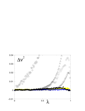
FIG. 2.: Difference $\Delta\nu^{2}$ of the reduced mode frequency between various model results and direct integration of the hydrodynamic equation. Open circles: zeroth order $\alpha-p$ model. Open up-triangles: sum rule method. Open squares: 3 parameters quasi-polynomial model with first estimator in Eq.(22). Open down-triangles: 3 parameters quasi-polynomial model with second estimator in Eq.(22). Filled circles: corrected $\alpha-p$ model. Filled squares: corrected 3 parameters quasi-polynomial model with first estimator in Eq.(22). Filled down-triangles: corrected 3 parameters quasi-polynomial model with second estimator in Eq.(22).

Making use of the 3 parameters quasi-polynomial model makes a very important improvement as can seen in Fig. 1 and 2. Indeed for $\lambda\begin{array}[]{c}<\vspace{-2,5mm}\\ \sim\end{array}0.4$ the results are within the noise of the direct integration, that is within $10^{-3}$ from the exact result. Then for higher $\lambda$ it starts to deviate with a maximum deviation of 0.03 for $\lambda=0.9$, then it gets back essentially to the exact value at the collapse.

For comparison we have also plotted on Fig. 1 and 2 the result from the sum rule method [9], which is basically a variational method. We have adapted it in the following way to our present problem. We start with the expression given by MS for the monopole frequency [4] $2\,\omega_{M}^{-2}=-d\,\ln\langle r^{2}\rangle/d\,\Omega^{2}$ (here we do not use the cloud radius as unit length). This relation is more conveniently expressed in terms of the oscillator length $l_{o}=\sqrt{\hbar/m\Omega}$ as:

$$\nu_{M}^{2} = 8\left(\frac{d\,\ln\langle r^{2}\rangle}{d\,l_{o}/l_{o}}\right)^{-1}$$ (25)

where, as above, $\nu_{M}^{2}=\omega_{M}^{2}/\Omega^{2}$ and the derivative is taken at constant number of particles $N$. Now, we express $\langle r^{2}\rangle$ as a function of $l_{o}$, $a$ and the coupling constant $\lambda$ defined above. In order to calculate $\langle r^{2}\rangle=\int\,d^{3}{\bf r}\,r^{2}\,n_{0}(r)$, we make in this integral the change of variables $t=k_{F}/k^{*}$ with $3\pi^{2}\,n_{0}(r)=k_{F}^{3}$ and $k^{*}=\pi/2|a|$. Using the equilibrium equation (24), we get $r^{2}=l_{o}^{4}\,k^{*\,2}\,P(\lambda,t)$, with $P(\lambda,t)=\lambda^{2}-t^{2}-\frac{2}{3}(\lambda^{3}-t^{3})$. After a straightforward calculation, we get:

$$\langle\,r^{2}\rangle = \frac{2}{3\pi}\,l_{o}^{10}\,k^{*\,8}\,F_{2}(\lambda)$$ (26)

$$N = \langle 1\rangle=\frac{2}{3\pi}\,l_{o}^{6}\,k^{*\,6}\,F_{0}(\lambda)$$ (27)

where $F_{q}(\lambda)=-\int_{0}^{\lambda}\,dt\,t^{3}\,P^{(q+1)/2}\,\partial P/\partial t$. From these two equations, we have:

$$d\,\ln\,\langle\,r^{2}\rangle = (F_{2}^{\prime}/F_{2})\,d\lambda\,+\,10\,\frac{dl_{o}}{l_{o}}$$ (28)

$$d\,\ln\,N = (F_{0}^{\prime}/F_{0})\,d\lambda\,+\,6\,\frac{dl_{o}}{l_{o}}$$ (29)

where $F_{q}^{\prime}=dF_{q}/d\lambda$. Since we take the derivative at constant $N$ in Eq.(25), we can eliminate $d\lambda$ from Eq.(28,29) and using Eq.(25), this yields:

$$\nu_{M}^{2} = \frac{4}{5-3\,F_{0}\,F_{2}^{\prime}/F_{0}^{\prime}F_{2}}$$ (30)

The calculation of $\nu_{M}^{2}$ (i.e the monopole frequency) therefore simply amounts to calculate four integrals. As it can be seen on Fig. 1 and 2, the sum rule method does remarkably well for $\lambda\begin{array}[]{c}<\vspace{-2,5mm}\\ \sim\end{array}0.4$ where it gives results within our direct integration noise. Then for larger $\lambda$ it starts to deviate and gets worse and worse when one goes to the collapse, where the deviation reaches 0.18. This is clearly linked [11] to the fact that the density has a linear dependence on $r$ at the collapse, as we have seen, while the sum rule method is best suited when there is a quadratic dependence at the center. In this respect one has to keep in mind that, even near the collapse for the trapped gas cloud as a whole, most of the gas has a density far from the one corresponding to the collapse of an homogeneous gas, because of the inhomogeneity caused by the trapping potential.

When we apply first order perturbative correction, as we have described above, we obtain a quite remarkable improvement. This is seen in Fig. 2 (the results have not been plotted in Fig. 1 since they would not be distinguishable from the direct integration ). Indeed the results we get from quasipolynomial modeling agree over the whole range of values for $\lambda$ with those of direct integration, within the numerical noise of $10^{-3}$. This is quite gratifying, but perhaps not completely unexpected, taking into account that we have three adjustable parameters, plus a correction. More surprising is that the corrected $\alpha-p$ model gives also results which are almost within numerical noise, though the quasipolynomial results are slightly better. Since without correction the quasipolynomial model is clearly much better, as it can be seen in Fig. 1, this excellent final agreement of the $\alpha-p$ model is perhaps partially coincidental, although we find the same feature in the next section for the 1D Bose gas.

It is clear that the excellent agreement within $10^{-3}$ of the results from the quasipolynomial and the $\alpha-p$ model gives us very much confidence in the validity of the result itself within this precision. We could ignore the direct integration and only infer the final result from what we obtain from the various models. This is naturally the point of view that we will adopt in the next section when we will study 1D bosons.

FIG. 3.: Lines of equal values in the $\alpha-p$ plane for the first of the estimators Eq.(22). Starting from the minimum which is at 3.10^-5, the black ellipse corresponds essentially to 3.10^-5,the dashed lines to 4.10^-5, 5.10^-5, 6.10^-5, 8.10^-5 and 9.10^-5 respectively for $I^{2}$. The band of open squares corresponds to the region where the reduced frequency calculated by the corrected $\alpha-p$ model is within $\pm$10^-3 from the direct integration. This band is also shown in Fig. 4.

In this respect, as we mentionned already, it is interesting to note that the first order perturbative correction takes essentially care of the difference which appears when we use different modeling and/or use different estimators and/or use different minima of these estimators. In particular, as we have already mentionned, if one requires very precise results, it is not always easy to locate the absolute minimum of an estimator. The use of the first order perturbative correction solves this problem since, as we have seen, the dispersion of the corrected results is very small compared to the one of the uncorrected ones. So we are allowed a little imprecision in the choice of the parameters of our modeling, since the first order perturbative correction will compensate for the resulting error in the mode frequency. It is naturally interesting to study this point in more details. We have done it for a worst case situation $\lambda=0.9$, a value near a maximal dispersion of the results as we have seen. We have only considered the $\alpha-p$ model in order to have only a two-dimensional parameter space. We have covered the range $1.15\leq\alpha\leq 1.4$ , $1.65\leq p\leq 1.9$. The lines of equal values for the first of the estimators Eq.(22) are drawn in Fig. 3. Since we are near the minimum these lines are elliptical. One sees that the minimum is quite shallow for the direction in the $\alpha-p$ plane corresponding to the large axis of these ellipses. We have also shown in this figure the region where the corrected $\alpha-p$ model gives a result within $\pm$10^-3 from the direct integration. It is quite satisfactory that this region goes very near the minimum of our estimator (the difference is basically within the noise) and is essentially oriented along the large axes of the ellipses (naturally we have generically a line in the $\alpha-p$ plane corresponding to any given value of $\nu^{2}$). Again for the corrected $\alpha-p$ model, we have plotted in Fig. 4 the lines of equal values for $\nu^{2}$ being respectively at $\pm$10^-3, $\pm$2.10^-3, $\pm$5.10^-3 and $\pm$7.10^-3 from the direct integration result $\nu^{2}=2.505$. We see that one can take values for ($\alpha,p$) which correspond to an estimator three times larger than the minimum and still obtain a result for $\nu^{2}$ which is at worst only within $\pm$5.10^-3 from the exact result. The corresponding value of the estimator shows that the average deviation between the model and the exact $\mu(n)$ is roughly $1\%$. This shows that, even with a modeling which is not very precise, we can obtain a very good result for $\nu^{2}$.

FIG. 4.: Lines of equal values in the $\alpha-p$ plane for $\nu^{2}$ being respectively at $\pm$10^-3(dotted line), $\pm$2.10^-3(short dashed-line), $\pm$5.10^-3(long dashed-line) and $\pm$7.10^-3(full thick line) from the direct integration result $\nu^{2}=2.505$. The full thin line corresponds to values in the $\alpha-p$ plane where the first order correction to the $\alpha-p$ model is actually zero.

When one sees the range of values for the parameters giving essentially the correct mode frequency, one may wonder if there is not another criterium than the above estimators to find a priori the best set of parameters. An interesting possibility in this direction is to say that the best parameters should not require any first order correction at all. So one should use sets of parameters giving zero correction. These sets correspond to a line in the $\alpha-p$ plane which is shown in Fig. 4. We have calculated the corresponding mode frequencies. We have found that, although the results are fairly independent of the parameter set, they fall systematically slightly above, at 2.514 , compared to the correct result 2.505 . Actually either of the estimators Eq.(22) turns out to be the best criterium to find the correct result (the difference between these two being within the numerical noise). This is seen in Fig. 2 where both estimators have been used.

VI THE 1D BOSE GAS

We apply now the previously developed method to study the hydrodynamic modes of the trapped 1D Bose gas with repulsive interactions. At zero temperature, the interactions are characterized by a single parameter: the 3D $s$-wave scattering length $a$. The system we consider is the same as the one studied by Menotti and Stringari [4]. Namely, this is a Bose gas in a very anisotropic trap ($\omega_{\perp}\gg\omega_{z}$) for various one-dimensional configurations. The transverse oscillator length $a_{\perp}=\sqrt{\hbar/m\omega_{\perp}}$ is supposed to be much larger than the scattering length $a_{\perp}\gg a$. As we mentionned already in the introduction, MS identified three limiting regimes corresponding physically to decreasing 1D densities $n_{1}(0)$ at the center of the trap. At high density ($n_{1}(0)a\gg 1$), the system is in the radial Thomas-Fermi regime (3D cigar). In this case the chemical potential is related [4] to the 1D density by $\mu=2\hbar\omega_{\perp}(an_{1})^{1/2}$, as indicated already in section III. In the second regime of intermediate densities, it is convenient to introduce the effective 1D scattering length $a_{1}$ related to the Lieb-Liniger coupling constant $g_{1}$ by $g_{1}=2\hbar^{2}/ma_{1}$. In the limit $a_{\perp}\gg a$, Olshanii [13] showed that $a_{1}=a_{\perp}^{2}/a$ [14]. In this intermediate density regime defined by $n_{1}(0)a_{1}\gg 1\gg n_{1}(0)a$, the gas is a 1D quasi-condensate (1D mean-field regime) and the chemical potential is given by $\mu=2\hbar\omega_{\perp}an_{1}$ (with our conventions $\mu$ is zero for zero density). Finally at low density $1\gg n_{1}(0)a_{1}$, the gas consists of impenetrable bosons (Tonks-Girardeau regime) where $\mu=\pi^{2}\hbar^{2}n_{1}^{2}/2m$.

Our needed input, in order to obtain the mode frequencies, is the equation of state $\mu(n_{1})$ for the homogeneous gas at zero temperature. For the transition between the 3D cigar and the 1D mean-field regimes (high density domain), it can be obtained from the numerical solution of the 3D Gross-Pitaevskii equation in a cylindrical geometry [4]. Actually, it appears that the numerical results [12] can be very well approximated analytically by:

$$\mu(n_{1})=\hbar\omega_{\perp}(\sqrt{1+4n_{1}a}-1)$$ (31)

This formula gives the exact behavior in the two limiting cases (3D cigar and 1D mean-field) defined above and interpolates very well in between (to better than $2\%$). In the following, we will use this approximate analytic expression which is easier to manipulate and avoids numerical problems encountered when the equation of state is only known for a fixed set of points. In the high density domain, we use the dimensionless variable $n_{1}(0)a$ to go from one regime to the other.

The equation of state for the transition between the 1D mean-field and Tonks-Girardeau regimes (low density domain) can be obtained from the Lieb-Liniger solution [6]. Lieb and Liniger gave a closed expression for the energy per particle as a function of the density in the form of an integral equation. It shows that the chemical potential is a universal function of $n_{1}a_{1}$, which has to be evaluated numerically. Menotti and Stringari [4] calculated this equation of state and made their result available [12]. In the following, we use their data. In the low density domain, the dimensionless variable we use is $n_{1}(0)a_{1}$.

Using these equations of state, we compute the mode frequency using the following procedure: for each value of $n_{1}(0)a$ (or $n_{1}(0)a_{1}$) we fit the equation of state (for $n_{1}$ varying between $0$ and $n_{1}(0)$) with an analytic model (either $\alpha-p$ or 3 parameters quasi-polynomial) using one of the estimator of equation (22); the zero order mode frequency is then obtained by inserting the value of the best set of parameters in the formula giving the mode frequency for the analytic model (Eq.(8) for the $\alpha-p$ model); we then compute the first order perturbation correction to the mode frequency.

We first discuss the different models used to compute the (squared) reduced mode frequency $\nu^{2}=\omega^{2}/\omega_{z}^{2}$. Fig. 5 shows $\nu^{2}$ as a function of $n_{1}(0)a$ for a system where $a_{\perp}/a=100$. Four curves are plotted. They correspond to the $\alpha-p$ model, the quasi-polynomial model, and to the same two models corrected to first order of perturbation theory. Actually, the 3 parameters quasi-polynomial model is used with only two parameters by fixing $\alpha=2$. We checked that, in the case of the 1D Bose gas and unlike that of the 3D Fermi gas, it does not make a significant difference to let the three parameters free or to set $\alpha=2$, whereas it is much faster and easier to work with only two parameters.

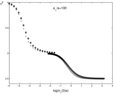
FIG. 5.: Lowest compressional mode of the trapped 1D Bose gas with $a_{\perp}/a=100$. The (squared) mode frequency $\nu^{2}=\omega^{2}/\omega_{z}^{2}$ is plotted as a function of $\log{(n_{1}(0)a)}$. The crosses ($+$) correspond to the $\alpha-p$ model; the stars ($\star$) to the corrected $\alpha-p$ model; the circles ($\circ$) to the quasi-polynomial model; and the diamonds ($\diamond$) to the corrected quasi-polynomial model. Actually at this scale all the symbols fall on top of each other, except for the crosses.

There are much more points plotted between the 3D cigar and the 1D mean-field regimes (high density domain) than between the 1D mean-field and the Tonks-Girardeau regime (low density domain). This is a mere consequence of the fact that we used an analytic expression for the equation of state in the first domain Eq.(31), whereas in the second one we used the numerical data of MS. Having a fixed set of points for the equation of state makes the numerical evaluation of integrals (needed to compute the correction $\delta\nu^{2}$, for example) more difficult because we are forced to use a primitive integration algorithm and, therefore, puts a limit on the precision and on the number of points that can be calculated safely. The fact that the junction between the two domains is not perfect (in the region of the 1D mean-field regime) is a consequence of taking a finite value for $a_{\perp}/a$ instead of the limit $a_{\perp}/a\rightarrow\infty$. As noted by MS, the 1D mean-field regime can only be identified provided $a_{\perp}/a\gg 1$.

In order to compare our various calculations, we look now at our results with a much larger scale, which amounts to using a magnifying glass. We take as reference the results of the corrected quasi-polynomial model. As discussed in the preceding section we expect this reference to be the best of our results and to be very precise. The difference between this reference and the three first calculations ($\alpha-p$, quasi-polynomial and corrected $\alpha-p$ models) are plotted in Fig. 6. Two points already made when discussing the 3D Fermi gas are worth stressing again in the case of the 1D Bose gas. First, once corrected, the results of the $\alpha-p$ and the quasi-polynomial models agree remarkably well. Second, their agreement is at the absolute $10^{-3}$ level for $\nu^{2}$.

The $\alpha-p$ model is exact in the three limiting regimes: $\alpha=2$ and $p=2$ in the 3D cigar regime, which gives $\nu^{2}=5/2$; $\alpha=2$ and $p=1$ in the 1D mean-field regime, which gives $\nu^{2}=3$; and $\alpha=2$ and $p=1/2$ in the Tonks-Girardeau regime, which gives $\nu^{2}=4$. In between these limits, it is apparent on Fig. 5 and 6 that the $\alpha-p$ model has some difficulties in predicting precisely the correct value of the mode frequency. This is what originally motivated the use of the 3 parameters quasi-polynomial model and the development of corrections using perturbation theory. This difficulty can actually be understood in much the same way as for the 3D Fermi gas. For example in the transition between the 3D cigar and the 1D mean field, one finds that for large $n_{1}(0)a$ one has essentially $\mu\sim n_{1}^{1/2}$ for most of the $n_{1}$ range, while for small $n_{1}$ this dependence turns into $\mu\sim n_{1}$. This switch of analytical behaviour is difficult to follow for the simple $\alpha-p$ model, hence the somewhat unsatisfactory result.

For the $\alpha-p$ and quasi-polynomial models, using an analytic expression for the equation of state (high density domain) gives better results than using numerical data (low density regime), as can be seen on Fig. 6. This is linked to the difficulty, mentionned above, of using purely numerical data as an entry for $\mu(n_{1})$. However, the corrected models agree at the same level in both domains.

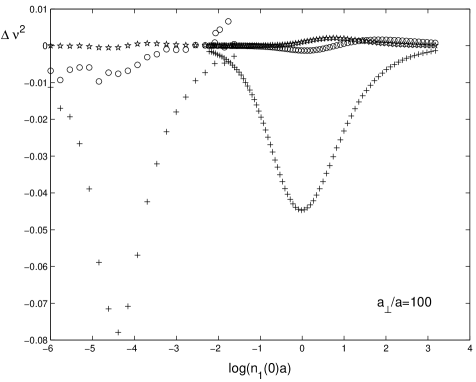
FIG. 6.: Lowest compressional mode of the trapped 1D Bose gas with $a_{\perp}/a=100$. The (squared) mode frequency $\nu^{2}=\omega^{2}/\omega_{z}^{2}$ calculated using the corrected quasi-polynomial model is taken as a reference. The difference between this reference and three different calculations ($\alpha-p$, corrected $\alpha-p$ and quasi-polynomial models) are plotted as a function of $\log{(n_{1}(0)a)}$. The crosses ($+$) correspond to the $\alpha-p$ model; the stars ($\star$) to the corrected $\alpha-p$ model; and the circles ($\circ$) to the quasi-polynomial model.

We will now compare our results with those of Ref. [4], first discussing the high density domain. Menotti and Stringari calculated $\nu^{2}$ as a function of $Naa_{\perp}/a_{z}^{2}$, where $a_{z}=\sqrt{\hbar/m\omega_{z}}$ is the longitudinal oscillator length and $N$ the number of particles. In this paper, we calculate the same quantity as a function of the more convenient $n_{1}(0)a$, which is an increasing function of $Naa_{\perp}/a_{z}^{2}$. Finding the relation between these two numbers amounts to obtaining the normalized density profile. This can be done analytically in the two limiting regimes [4] and numerically in between. This allows to plot the MS result for the mode frequency and our corrected quasi-polynomial result (which we expect to be the most precise of our results) on the same graph, see Fig. 7. It shows excellent agreement, at the $10^{-2}$ level. Asking for agreement at a better level is not sensible here, as we used an analytic expression approximating the equation of state within a few percent and not the exact equation of state. This shows up in the fact that for high densities ($n_{1}(0)a>1$), the corrected quasi-polynomial seems to predict values of the mode frequency that are higher than the result of MS. This would be in contradiction with the fact that the sum rule approach they used is known to be an exact upper bound [9].

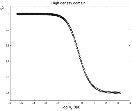
FIG. 7.: Lowest compressional mode of the trapped 1D Bose gas in the high density domain. The (squared) mode frequency $\nu^{2}=\omega^{2}/\omega_{z}^{2}$ is plotted as a function of $\log{(n_{1}(0)a)}$. The diamonds ($\diamond$) correspond to the corrected quasi-polynomial model. The full line is the result of Menotti and Stringari.

As a further check on our method, we also calculated the expected frequency for two experiments. For this purpose, the exact equation of state was used, in the form of the numerical solution of the 3D Gross-Pitaevskii equation [12]. For the experiment of Ref. [15], where $n_{1}(0)a=0.22$, we find $\nu^{2}=2.845\pm 0.003$ and $\nu^{2}=2.911\pm 0.002$ for the experiment of Ref. [16], where $n_{1}(0)a=0.10$. This is in complete agreement with the values first obtained by MS.

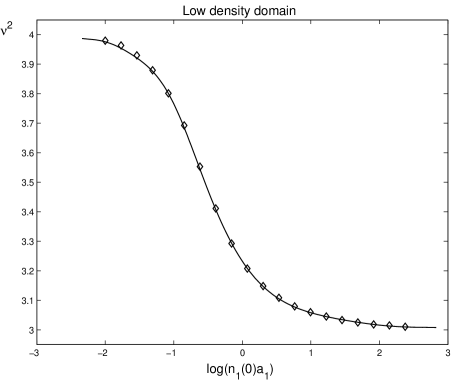
FIG. 8.: Lowest compressional mode of the trapped 1D Bose gas in the low density domain. The (squared) mode frequency $\nu^{2}=\omega^{2}/\omega_{z}^{2}$ is plotted as a function of $\log{(n_{1}(0)a_{1})}$. The diamonds ($\diamond$) correspond to the corrected quasi-polynomial model. The full line is the result of Menotti and Stringari.

We consider finally the low density domain. As in the high density domain, we first have to relate the dimensionless variable we use $n_{1}(0)a_{1}$ to $Na_{1}^{2}/a_{z}^{2}$ used in Ref. [4]. This is done analytically in the 1D mean-field and in the Tonks-Girardeau regime [4] and numerically in between. The mode frequency obtained by the corrected quasi-polynomial model and that calculated by MS are plotted in Fig. 8. The agreement is again very good.

The results of MS are in very good agreement with our result over the whole range of $n_{1}(0)a$. In the case of the 1D Bose gas, the sum rule approach [9] seems to give not only an upper bound but to be quite near the exact result. As already discussed in the case of 3D Fermi gas, this is related to the fact that the density has a quadratic dependence on $r$ near the center of the trap. In other words, the parameter $\alpha$ is always very close to $2$.

VII CONCLUSION

In this paper we have calculated, as a function of density at the center of the trap, the frequency of the lowest compressional mode of a 1D trapped Bose gas, taking the reactive hydrodynamic equations as a starting point. We have considered two density regimes. In the first one the density decreases from high to intermediate, but the Bose gas is always described microscopically by 3D mean field theory. In the high density region the Bose gas has the shape of a 3D cigar, while in the intermediate density region the atoms are in the one-particle ground state with respect to the transverse motion and the gas behaves as a 1D system. Nevertheless for all this regime the low frequency modes are described by 1D hydrodynamic equations, but the effective equation of state Eq.(31) is no longer given by mean field. The second regime that we have considered goes from intermediate to low density and we have taken the Lieb-Liniger model to describe it, which corresponds to a 1D Bose gas going from a weakly to a strongly interacting situation.

In order to solve the hydrodynamic equations we have made use of a very recent approach which allows to find analytical or quasi-analytical solutions of these equations for a large class of models. These model solutions allow to approximate very nearly the exact equation of state which is the only input of the hydrodynamic equations coming from the physical properties of the system. When in addition a first order correction has been made, we have been able to check that this method gives the correct mode frequency with at least a relative precision of $10^{-3}$ which is more than necessary for any practical purpose. On the other hand the simplest of this model gives a very easy and convenient analytical solution. Taken together the ensemble of these models allow to cover all the range from simple analytical solutions to very precise numerical solutions. We have compared our results to those obtained by Menotti and Stringari from a sum rule approach, and we have found an excellent agreement.

The method used in this paper is quite powerful. It is not restricted to the lowest frequency mode and it can be used as well for any higher frequency mode. We have not presented the corresponding results in the present paper only to avoid to make it oversized, but this would have been quite easy. Another interest of our method is that it is not restricted to mean field and can be applied to any equation of state corresponding possibly to a very dense Bose gas. For example we could very well consider the situation where the gas is dense enough so that the 1D intermediate density situation can no longer be described by mean field [17, 18]. Moreover the convenience of analytical solutions makes it possible to invert the method [8] and to extract the effective equation of state of the gas from experimental data on the variation of the modes frequencies as a function of the density.

We acknowledge numerous conversations with Y. Castin, C. Cohen-Tannoudji, J. Dalibard, D. Gangardt and C. Salomon. We are extremely grateful to Sandro Stringari and Chiara Menotti for many stimulating discussions and for providing us with their data.

* Laboratoire associé au Centre National de la Recherche Scientifique et aux Universités Paris 6 et Paris 7.

REFERENCES

- [1] F. Dalfovo, S. Giorgini, L. P. Pitaevskii and S. Stringari, Rev. Mod. Phys. 71, 463 (1999) and references therein; C. Cohen-Tannoudji, cours du collège de France, http://www. ens.fr/cct
- [2] J.R. Anglin and W. Ketterle, Nature 416, 211 (2002).
- [3] E. A. Donley, N. R. Claussen, S. T. Thompson and C. E. Wieman, Nature 417 529 (2002).
- [4] C. Menotti and S. Stringari, Phys. Rev. A 66, 043610 (2002)
- [5] E.P. Gross, Nuovo Cimento 20, 454 (1961); L.P. Pitaevskii, J. Exp. Theor. Phys. 40, 646 (1961).
- [6] E.H. Lieb, W. Liniger, Phys. Rev. 130, 1605 (1963).
- [7] L. Tonks, Phys. Rev. 50, 955 (1936); M. Girardeau, J. Math. Phys. 1, 516 (1960).
- [8] R. Combescot and X. Leyronas, Phys.Rev.Lett.89, 190405 (2002).
- [9] S. Stringari, Phys.Rev.Lett.77 2360 (1996).
- [10] S. Stringari, Phys.Rev. A 58, 2385 (1998).
- [11] We are very grateful to Sandro Stringari for this point.
- [12] We thank Chiara Menotti for providing us with her data.
- [13] M. Olshanii, Phys. Rev. Lett. 81, 938 (1998).
- [14] We follow Menotti and Stringari [4] in the definition of the effective 1D scattering length. There is a difference in sign with the definition of Olshanii [13].
- [15] A. Görlitz et al., Phys. Rev. Lett. 87, 130402 (2001).
- [16] F. Schreck et al., Phys. Rev. Lett. 87, 080403 (2001).
- [17] G.E. Astrakharchik and S. Giorgini, Phys. Rev. A 66, 053614 (2002).
- [18] D.Blume, Phys. Rev. A 66, 053613 (2002).