[

Nanoscale Phase Coexistence and Percolative Quantum Transport

Abstract

We study the nanoscale phase coexistence of ferromagnetic metallic (FMM) and antiferromagnetic insulating (AFI) regions by including the effect of AF superexchange and weak disorder in the double exchange model. We use a new Monte Carlo technique, mapping on the disordered spin-fermion problem to an effective short range spin model, with self-consistently computed exchange constants. We recover ‘cluster coexistence’ as seen earlier in exact simulation of small systems. The much larger sizes, $\sim 32\times 32$, accessible with our technique, allows us to study the cluster pattern for varying electron density, disorder, and temperature. We track the magnetic structure, obtain the density of states, with its ‘pseudogap’ features, and, for the first time, provide a fully microscopic estimate of the resistivity in a phase coexistence regime, comparing it with the ‘percolation’ scenario.

]

The issue of multiphase coexistence in transition metal oxides has been brought to the fore by a set of remarkable recent experiments on the manganites [1, 2]. These experiments probe the atomic scale magnetic correlations [3], structural features [4], or ‘conducting’ properties, i.e tunneling density of states [5], through local spectroscopy. The bulk thermodynamic and transport properties of these systems, including the ‘colossal magnetoresistance’ (CMR) seem to have a correlation with the physics of electronic phase coexistence as visualised in these nanoscale experiments.

Establishing a first principles theoretical connection between cluster coexistence and ‘anomalous’ transport, however, has been difficult. Only real space Monte Carlo (MC) techniques [6] allow access to the cluster phase, and accessible sizes, $\sim 8\times 8$ in two dimension (2d), are too small to study transport. The approach in current use [7] is phenomenological, using classical resistor networks to model the data within a ‘percolation scenario’. While ‘percolation’ surely plays an important role in transport, standard percolation theory [8] is inadequate [9] to explain the data. More fundamentally, such an approach does not explain the temperature and field dependent resistance of the ‘building blocks’, or correlations and hysteresis in the cluster distribution, or the dependence of bulk resistance on ‘spin overlap’ between clusters.

We address these questions within a ‘spin-fermion’ model in this paper, employing a new MC technique [10] that allows access to system sizes $\sim 32\times 32$ in 2d. This can probe the regime $L_{S}\gg{\bar{L}_{c}}\gg a_{0}$, where $L_{S}$, ${\bar{L}_{c}}$ and $a_{0}$ are system size, typical cluster size, and lattice spacing, respectively. We study the coexistence regime, obtain the typical cluster size, and calculate the spectral density and conductivity in the mixed phase. To our knowledge this is the first microscopic calculation to clarify the connection between nanoscale phase coexistence and transport in a fully quantum mechanical itinerant electron system.

The coexistence of two phases with distinct electronic, magnetic, and possibly structural, properties is best conceived at $T=0$ in a clean system. For a specified chemical potential, $\mu$, the ground state configuration of the spin and lattice variables, $\{X_{i}\}$ say, assumed classical, is determined by $\delta{\cal E}/{\delta X_{i}}=0$, where ${\cal E}\{X_{i};\mu\}$ is the energy of the system in the $\{X_{i}\}$ background. The minimum, ${\cal E}_{min}(\mu)$, usually occurs for a unique $\{X_{i}\}$ at each $\mu$, and in this background the electron density $n(\mu)$ is also unique. However, in the presence of competing interactions, two distinct $\{X_{i}\}$ configurations could be degenerate minima of ${\cal E}$ at some $\mu$. The corresponding $\mu=\mu_{c}$ marks a first order phase boundary, and the two ‘endpoint’ densities, $n_{1}$ and $n_{2}$ bracket a region of coexistence. There is no homogeneous phase with density between $n_{1}$ and $n_{2}$. In this regime the system breaks up into two macroscopic domains, with density $n_{1}$ and $n_{2}$.

It was pointed out by Dagotto and coworkers [6], and known earlier in the context of classical spin models [11], that disorder is a singular perturbation in these systems. Even weak disorder breaks up the ‘macroscopic’ domains into interspersed locally ordered clusters of the two phases. This nano/mesoscopically inhomogeneous strongly correlated phase can be studied only within a real space framework.

In this paper we study the key qualitative issues of phase coexistence in itinerant fermion models by considering the competing effects of double exchange (DE) and superexchange (SE) in the presence of weak disorder. We consider $H=H_{el}+H_{AF}$ in 2d, with:

$$H_{el}=\sum_{\langle ij\rangle\sigma}t_{ij}c^{\dagger}_{i\sigma}c^{~{}}_{j\sigma}+\sum_{i}(\epsilon_{i}-\mu)n_{i}-J_{H}\sum_{i}{\bf S}_{i}{\bf.}{\vec{\sigma}}_{i}$$ (1)

and $H_{AF}=J_{S}\sum_{\langle ij\rangle}{\bf S}_{i}.{\bf S}_{j}$. The hopping $t_{ij}=-t$ for nearest neighbours, and $\epsilon_{i}$ is uniformly distributed between $\pm\Delta/2$. We assume $J_{H}/t\rightarrow\infty$. The parameters in the problem are $\Delta/t$, $J_{S}/t$ and density $n$ (or chemical potential $\mu$). We use $|{\bf S}_{i}|=1$. For $J_{H}/t\rightarrow\infty$, the Hamiltonian, in the projected basis [10], assumes a simpler form: $H_{el}=-t\sum_{\langle ij\rangle}f_{ij}(~{}e^{i\Phi_{ij}}\gamma^{\dagger}_{i}\gamma_{j}+h.c~{})+\sum_{i}(\epsilon_{i}-\mu)n_{i}$. The hopping amplitude, $g_{ij}=f_{ij}e^{i\Phi_{ij}}$, between locally aligned states, can be written in terms of the polar angle $(\theta_{i})$ and azimuthal angle $(\phi_{i})$ of the spin ${\bf S}_{i}$ as, $cos{\theta_{i}\over 2}cos{\theta_{j}\over 2}$ $+sin{\theta_{i}\over 2}sin{\theta_{j}\over 2}e^{-i~{}(\phi_{i}-\phi_{j})}$. The ‘magnitude’ of the overlap is $f_{ij}=\sqrt{(1+{\bf S}_{i}.{\bf S}_{j})/2}$, while the phase is specified by $tan{\Phi_{ij}}=Im(g_{ij})/Re(g_{ij})$.

To make progress we need the ‘effective Hamiltonian’ controlling the Boltzmann weight for the spins. Formally, this is: $H_{eff}\{{\bf S}_{i}\}=-(1/\beta)logTre^{-{\beta}(H_{el}+H_{AF})}$. The ‘exact’ MC directly generates equilibrium spin configurations of $H_{eff}$ through iterative diagonalisation [6]. We make the approximation: $H_{eff}=-\sum_{\langle ij\rangle}D_{ij}f_{ij}+J_{S}\sum_{\langle ij\rangle}{\bf S}_{i}.{\bf S}_{j}$, with $D_{ij}$ being determined self consistently [10] as the average of ${\hat{\Gamma}}_{ij}=(e^{i\Phi_{ij}}\gamma^{\dagger}_{i}\gamma_{j}+h.c)$ over the assumed equilibrium distribution. This approximation has been extensively benchmarked for the clean DE model [10] and we will put up similar comparisons for the present problem in the near future [12].

Although the $D_{ij}$ enter as ‘nearest neighbour’ exchange, they arise from a solution of the full quantum statistical problem in the disordered finite temperature system. In the presence of competing interactions and quenched disorder, this leads to a set of strongly inhomogeneous, spatially correlated, and temperature dependent ‘exchange’ $D_{ij}$.

At consistency, fermionic properties are computed and averaged over equilibrium spin configurations. We work

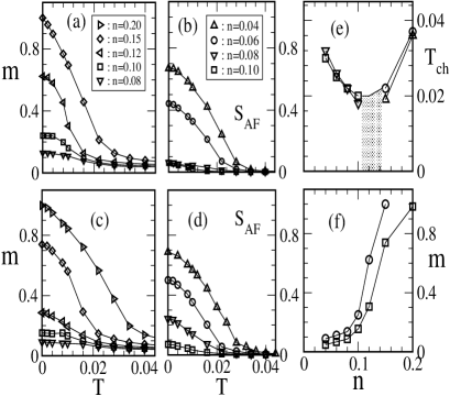
FIG. 1.: Magnetisation, $m(T)$, and structure factor, $S_{\bf q}(T)$ at ${\bf q}=\{\pi,\pi\}$. Panel $(a)-(b)$: data for $\Delta=0.2$, panel $(c)-(d)$: data for $\Delta=1.0$. The legends are common to panels $(a)-(d)$. Panel $(e)$: The characteristic temperature (see text), $T_{ch}(n,\Delta)$: triangle down: AF at $\Delta=1.0$, square: AF at $\Delta=0.2$, triangle up: FM at $\Delta=1.0$, circles: FM at $\Delta=0.2$. Panel $(f)$: $m(T=0)$ with varying $n$, circles: $\Delta=0.2$, squares: $\Delta=1.0$. System size: $24\times 24$.

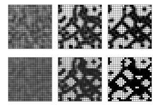
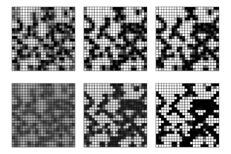
FIG. 2.: Cluster pattern: Rows 1-2 are for $\Delta=0.2$, row 3-4 are for $\Delta=1.0$. Mean density $n=0.1$ in both cases. Upper row in each set shows the thermally averaged density profile, $n_{\bf r}$, the lower row shows the nearest neighbour spin correlation: $f_{2}^{s}=\langle{\bf S}({\bf r}).{\bf S}({\bf r}+{\bf\delta})\rangle$. Left to right along each row, the $T$ variation is $T/T_{c}\sim 2.0,1.0,0.0$. For $n_{\bf r}$ dark regions are high density. For $f_{2}^{s}$ dark regions are FM, white regions AF. System size $32\times 32$, data for a specific $\{\epsilon_{i}\}$ in each case.

at specified mean density, fixing $\mu$ through iteration. Transport properties are computed using the Kubo formula [10], employing sizes $\sim 24\times 24$ to $32\times 32$, and averaged typically over $30$ realisations of disorder, with averaging over $\sim 50$ equilibrium spin configurations at each $T$ for each realisation of $\{\epsilon_{i}\}$. Since the d.c conductivity is not directly accessible in a finite system, we compute the finite frequency conductivity at the scale of mean level spacing, $\omega_{L}\propto 8t/L^{2}$, with $\omega_{L}=0.04t$ at $L=32$. The conductivity results are in units of $(\pi e^{2})/{\hbar}$. We have checked the adequacy of disorder average and stability with respect to system size variation [12].

Our principal results include the direct visual evidence of cluster coexistence (Fig.2), the disorder dependence of spectral density (Fig.3) and the resistivity (Fig.4) in the coexistence regime.

At low electron density, the competetion in the DE$+$SE model is between a $\{\pi,\pi\}$ AF phase and a ferromagnet (FM). We set $J_{S}=0.05$ and scanned in $\mu$ to locate the $\mu_{c}$ for the first order boundary. The density changes from $n=0$ to $n\sim 0.20$ at the discontinuity. These results were obtained within the $H_{eff}$ scheme and cross checked with exact MC. Moderate disorder smooths out the discontinuity in $n(\mu)$ converting it to a sharp crossover [12]. In this paper we fix $J_{S}=0.05$ and probe the coexistence regime, $n\sim 0-0.2$, with varying electron density, temperature $(T)$, and $\Delta=0.2$ and $\Delta=1.0$. All the results are obtained by cooling the system from the high $T$

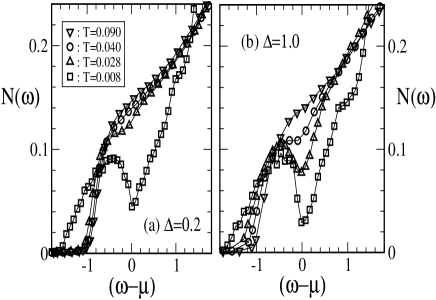
FIG. 3.: Low energy density of states, at $n=0.10$. Panel $(a)$: data at $\Delta=0.2$, panel $(b)$: data at $\Delta=1.0$. The DOS is plotted with respect to $\omega-\mu(T)$, incorporating the $T$ dependent shift in $\mu$. Lorentzian broadening of $\delta$ functions to $0.03$. Data averaged over 30 copies.

paramagnetic, approximately homogeneous, phase.

Fig.1 shows the magnetisation, $m(T)$, and the AF peak in the magnetic structure factor $S_{\bf q}$ at ${\bf q}=\{\pi,\pi\}$ to illustrate the evolution from the AF to the FM phase with increasing $n$. Panel $(a)-(b)$ are at $\Delta=0.2$ and panel $(c)-(d)$ at $\Delta=1.0$. The ‘extremal’ densities are either strongly AF or FM, while for $n\sim 0.08-0.12$ both FM and AF reflections have finite weight. Panel $(e)$ tracks the ‘characteristic temperature’, $T_{ch}(n,\Delta)$, identified from the maximum in ${\partial^{2}O}/{\partial T^{2}}$ where $O$ is the appropriate order parameter (of the FM or AF phase). In the shaded region, $0.10\lesssim n\lesssim 0.14$, it is difficult to resolve the $T_{ch}$ accurately. Panel $(f)$ shows the change in ‘saturation magnetisation’ $m(T=0)$ with increasing $n$ and changing disorder. The small moment regime, $m\lesssim 0.1$, for $n\lesssim 0.1$ is a ‘ferro-insulator’ phase, as we will discover from the transport data. In this regime the moments in different clusters are only weakly correlated.

Fig.2 provides direct visual evidence of ‘clustering’, the top two panels showing thermally averaged local density and nearest neighbour spin correlation for $T/T_{c}\sim 2.0,1.0,0.0$ (left to right), at $\Delta=0.2$. The lower panels show data at $\Delta=1.0$. We will quantify the ‘typical scale’ of clusters later, but from the density distribution it is obvious that the pattern for $\Delta=1.0$ is more fragmented than for $\Delta=0.2$. The ‘density contrast’ reduces with increasing $T$, as the spins in the AF regions fluctuate out of antiparallel alignment, and the carriers can partially explore these regions. The spin correlations also weaken, with FM (black) and AF (white) regions giving way to an uncorrelated (grey) background.

Fig.3 shows the low energy density of states (DOS) for $n=0.1$. Even at weak disorder, panel $(a)$, there is a ‘pseudogap’ in the system averaged DOS, at the lowest temperature, $T\sim 0.01$. However, the pseudogap rapidly fills up with increasing $T$, and the DOS tends towards

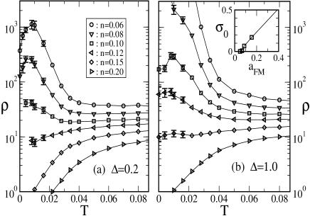
FIG. 4.: Resistivity, $\rho(T)$, with varying $n$. Panel $(a)$: $\Delta=0.2$, panel $(b)$: $\Delta=1.0$. Results obtained on ‘cooling’. System size $24\times 24$, data obtained by inverting the ‘mean conductivity’. Average over $20-50$ copies of $\{\epsilon_{i}\}$ (error bars comparable to symbol size, unless otherwise indicated). Results on size $32\times 32$ are similar. Inset, panel $(b)$: Normalised $T=0$ conductivity, at $\Delta=1$, -vs- FMM surface area.

the universal profile of the spin disordered 2d DE model. At stronger disorder, panel $(b)$, the ‘dip’ in the DOS at $\mu$ is deeper. Due to stronger pinning, the clusters, and the gap feature, survives to higher $T$, and only for $T\gg T_{ch}$ tends to the asymptotic form. While this data focuses on the system averaged DOS, which can be probed by photoemission (PES), tunneling spectroscopy would track the local DOS, which shows [12] a clean ‘gap’ in the AF regions, and finite DOS in the (larger) metallic clusters.

Fig.4 shows resistivity, $\rho(T)$, with varying $n$ and disorder. The comparison of panel $(a)$, $\Delta=0.2$, and panel $(b)$, $\Delta=1.0$, indicates that $\rho(T)$ for stronger disorder is systematically larger. The trends, however, are similar in the two cases and allows a tentative classification of the ‘global’ aspects of transport. At both $\Delta=0.2$ and $\Delta=1.0$ there is a critical density, $n_{c}(\Delta)$, below which $\rho(T=0)$ diverges, indicating the absence of any connected ‘conducting path’. The inset to panel $(b)$ shows the trend in the $T=0$ conductivity with increasing FM cluster area, $a_{FM}$.

We suggest the following qualitative picture of transport in the coexistence regime based on the data in Fig.4. $(a)$. At low $T$, and for $n>n_{c}(\Delta)$, there is, by definition, some connected ‘metallic path’ through the sample. It is reasonable to assume that at least in this connected region the spins are aligned due to DE. Since cluster dimension and electron wavelength are comparable in our system a large fraction of the resistance arises from the non trivial geometry of the current path. This scattering is quantum mechanical, and the low $T$ metallic phase corresponds to a quantum percolative regime [13], for roughly $0.15\gtrsim n\gtrsim 0.08$ at $\Delta=1.0$. $(b)$. With increasing $T$, the resistance of the conducting network increases due to DE spin fluctuations and, till the network is disrupted, there

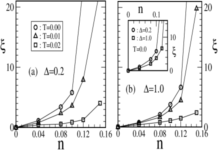
FIG. 5.: Typical FMM cluster size: $(a)$ $\Delta=0.2$ and varying $T$, $(b)$ $\Delta=1.0$, varying $T$. The inset to panel $(b)$ highlights the reduction in cluster size with increasing disorder.

is a regime $d\rho/dT>0$. This ‘metallic’ behaviour occurs despite the very large residual resistivity. This is a regime of weak magnetic scattering on the conducting network. If $n\gg n_{c}$, e.g, $n=0.20$ in Fig.4.$(b)$, so that inhomogeneities are weak, $\rho(T)$ will smoothly increase to the $T\gg T_{ch}$ asymptotic value. $(c)$. With further increase in $T$, in the $n\gtrsim n_{c}$ regime, the spin disorder can destroy some of the ‘weak links’, disrupting the conducting network and leading to a sharp increase in $\rho(T)$ see, e.g, $n=0.1$ in Fig.4.$(b)$. This correlates well with reduction in typical cluster size with increasing $T$, discussed in the next paragraph. Depending on $n$ and the extent of disorder (and system size, in a simulation) there could be a rapid rise or a ‘first order’ metal-insulator transition (MIT). This is spin disorder induced breakup of clusters driving a MIT. $(d)$.  Beyond this ‘MIT’ the conduction is through the ‘insulating’ regions, with isolated patches contributing to nominally activated transport, as visible in Fig.4.$(b)$ for $n\lesssim 0.12$. For $T\gg T_{ch}$, as the structures disappear, Fig.2, and the system becomes homogeneous, $\rho(T)$ is dominated by spin disorder scattering. This is a diffusive regime with saturated spin disorder scattering, visible for $T\gtrsim 0.08$ at all densities. $(e)$. For $n<n_{c}$, the regime of low density isolated clusters, $\rho(T)$ falls monotonically, and the response is typical of low density ferromagnetic polarons in a AF background. This occurs for $n\lesssim 0.08$ at $\Delta=1.0$, and at lower $n$ at $\Delta=0.20$.

Finally, Fig.5 shows the typical size of FMM clusters, inferred from a Lorentzian fit to the magnetic structure factor, i.e, $S_{\bf q}\sim(q^{2}+\xi^{-2})^{-1}$. The resulting correlation length depends on $n$, $\Delta$ and $T$, decreasing with increasing disorder and $T$, and increasing with increasing density. The main panels, $(a)$ and $(b)$, highlight the $n$ dependence at different $T$ and $\Delta$, while the inset in Fig.5.(b) replots the same data to highlight the dependence on disorder. The dependences, overall, are intuitive, and strengthen the proposed transport scenario.

Our results on coexistence share several generic features with the manganites [3, 4, 5], but there are key differences too. Apart from the difference between 2d and 3d, these are $(i)$ the important regime of coexistence in manganites is between FMM and charge ordered insulator (COI), and crucially involves the Jahn-Teller (JT) phonons. This requires enlarging our model. $(ii)$ It is supposed that the FMM and COI regions are nominally of equal density, which is why such domains can survive over $\mu$m scale. Our clusters are ‘charged’ due to the density difference between FMM and AFI. In any real system Coulomb effects [14] would have to be considered in such a case. We will discuss such effects separately [12], as well as the effect of an applied magnetic field on transport.

In conclusion, we have presented microscopic results on quantum transport across a regime of phase coexistence in an itinerant fermion model, and correlated it with thermal evolution of the spatial structures. The method readily generalises to the two orbital model with JT phonons, to be discussed in the near future.

We acknowledge use of the Beowulf cluster at H.R.I

REFERENCES

- [1] N. Mathur and P. B. Littlewood, Solid. State. Commun. 119, 271 (2001).
- [2] E. Dagotto, T. Hotta and A. Moreo, Phys. Repts. 344, 1 (2001).
- [3] L. Zhang, C. Israel, A. Biswas, R. L. Greene and A. de Lozanne, Science, 298, 805 (2002).
- [4] M. Uehara, S. Mori, C. H. Chen and S. -W. Cheong, Nature, 399, 560 (1999), Ch. Renner, G. Aeppli, B. G. Kim, Y. Soh and S. -W. Cheong, Nature, 416, 518 (2002).
- [5] M. Fath, S. Freisem, A. A. Menovsky, Y. Tomioka, J. Aarts and J. A. Mydosh, Science, 285, 1540 (1999).
- [6] A. Moreo, M. Mayr, A. Feiguin, S. Yunoki and E. Dagotto, Phys. Rev. Lett. 84, 5568 (2000).
- [7] M. Mayr, A. Moreo, J. A. Verges, J. Arispe, A. Feiguin and E. Dagotto, Phys. Rev. Lett. 86, 135 (2000).
- [8] D. Stauffer and A. Aharony, Introduction to Percolation Theory, Taylor & Francis, London (1991).
- [9] J. Burgy, E. Dagotto and M. Mayr, Phys. Rev. B 67, 014410-1 (2003).
- [10] S. Kumar and P. Majumdar, cond-mat 0305345.
- [11] Y. Imry and S. K. Ma, Phys. Rev. Lett. 35, 1399 (1975), M. Aizenmann and J. Wehr, Phys. Rev. Lett. 62, 2503 (1989).
- [12] S. Kumar and P. Majumdar, to be published.
- [13] A quantum ‘random bond’ model, with ‘metallic’ and ‘insulating’ links, in 2d, is expected to be insulating, see Y. Avishai and J. M. Luck, Phys. Rev. B 45, 1074 (1992), but we do not know of any exact results in the context of ‘correlated bonds’ as relevant here.
- [14] K. Yang, Phys. Rev. B 67, 092201-1 (2003).