Two-dimensional delta potential wells and condensed-matter physics

Abstract

It is well-known that a delta potential well in 1D has only one bound state but that in 3D it supports an infinite number of bound states with infinite binding energy for the lowest level. We show how this also holds for the less familiar 2D case, and then discuss why this makes 3D delta potential wells unphysical as models of interparticle interactions for condensed-matter many-body systems. However, both 2D and 3D delta wells can be “regularized” to support a single bound level which in turn renders them conveniently simple single-parameter interactions, e.g., for modeling the pair-forming dynamics of quasi-2D superconductors such as the cuprates, or in 3D of other superconductors and of neutral-fermion superfluids such as ultra-cold trapped Fermi gases.

PACS numbers: 03.75.Ss; 03.65.-w; 03.65.Ge; 74.78.-w
Key words: delta potential wells, bound states, regularization, condensed-matter physics.

Resumen

Es bien sabido que un pozo de potencial delta en 1D tiene un solo estado ligado pero que en 3D tiene un número infinito de estos estados con una energía de “amarre” infinita para el nivel más bajo. Aquí mostramos cómo esto también ocurre para el caso bidimensional que es menos familiar, para luego discutir por que los pozos de potencial delta en 3D no son físicos como modelos de interacciones entre partículas para sistemas de muchos cuerpos en materia condensada. No obstante, ambos pozos delta en 2D y 3D pueden ser regularizados para soportar un solo nivel ligado lo cual los convierte convenientemente en interacciones de un solo parámetro, por ejemplo, para modelar la dinámica de formación de pares en superconductores casi-bidimensionales tales como los cupratos, o en 3D la formación de pares en otros superconductores y en superfluidos fermiónicos neutros tales como los gases de Fermi atrapados ultrafríos.

I. INTRODUCTION

The study of physical systems in dimensions lower than three has recently shed its purely academic character and become a real necessity to describe the properties of novel systems such as nanotubes [1], quantum wells, wires and dots [2, 3], the Luttinger liquid [3, 4], etc. Reduced dimensionality describes superconducting phenomena in quasi-2D cuprates where pairing between electrons (or holes) is essential [5]. Whatever the actual interaction between two electrons (or holes) in a cuprate might ultimately turn out to be, the attractive delta potential is a conveniently simple model to visualize and to account for pairing, an indispensable element for superconductivity and neutral-fermion superfluidity. It enormously simplifies calculations. Bound states in a delta potential well in 1D and 3D are usually discussed in textbooks, but not in 2D. Refs. [6] and [7] discuss this from a more rigorous mathematical viewpoint without explicitly solving the Schrödinger equation, e.g., for the bound energy levels. Here, this gap is filled by analyzing the 2D time-independent Schrödinger equation with a delta potential well that is then “regularized” [8] to reduce its infinite bound levels to only one. The single-bound-level case suffices for now since, e.g., the well-known simple Cooper/BCS model interaction [9] mimicking the attractive electron-phonon pair-forming mechanism, but requiring two parameters (a strength and a cutoff) instead of the regularized $\delta$-potential’s only one (a strength), can also be shown to support a single bound state [10] in the vacuum or two-body limit. Were it not for the (momentum-space) cutoff parameter, the Cooper/BCS interaction in coordinate space would also be a $\delta$-potential, and indeed becomes such as the cutoff is properly taken to infinity.

From elementary quantum mechanics we first recall the bound-state energies $E<0$ in a potential “square” well of depth $V_{0}$ and range $a$, a common textbook example studied in 1D [11] and 3D [12]. In 1D the ground-state energy $E_{0}$ of a particle of mass $m$ can be expanded for small $V_{0}a$ as

$$E_{0}\;{\smash{\mathop{\relbar\joinrel\longrightarrow}\limits_{V_{0}a\to 0}}}\;-\frac{2ma^{2}V_{0}^{2}}{\hbar^{2}}+O\left(a^{3}V_{0}^{3}\right).$$ (1)

Thus, in 1D there is always at least one bound state no matter how shallow and/or short-ranged the well. Similarly, in 3D for a spherical well, an expansion of $E_{0}$ in powers of $\eta\equiv V_{0}a^{2}-\hbar^{2}\pi^{2}/8m$ $\geq 0$ gives

$$E_{0}\;{\smash{\mathop{\relbar\joinrel\longrightarrow}\limits_{\eta\to 0^{+}}}}\;\ \frac{m\eta^{2}}{2\hbar^{2}a^{2}}+O\left(\eta^{3}\right).$$ (2)

Thus, in contrast to 1D, a minimum critical or threshold value for $V_{0}a^{2}$ of $\hbar^{2}\pi^{2}/8m$ is needed in 3D for the first bound state to appear. Clearly, both 1D and 3D cases are perturbative expansions in an appropriate “smallness” parameter, $V_{0}a$ or $\eta$. As in 1D, a 2D circularly symmetric well of depth $V_{0}$ and radius $a$ always supports a bound state, no matter how shallow and/or short-ranged the well. However, this instance is non-perturbative as it gives [13] for the lowest bound-state energy

$$E_{0}\;{\smash{\mathop{\relbar\joinrel\longrightarrow}\limits_{V_{0}a^{2}\to 0}}}\;\ \frac{\hbar^{2}}{2ma^{2}}\exp\left(-\frac{2\hbar^{2}}{mV_{0}a^{2}}\right)$$ (3)

which cannot be expanded in powers of small $V_{0}a^{2}$ since it is of the form $f(\lambda)=e^{-1/\lambda}\mathrel{\mathop{\longrightarrow}\limits_{\lambda\rightarrow 0}}0,$ i.e., has an essential singularity at $\lambda=0$.

In this paper we discuss how, just as in the better known 3D case, the 2D potential well $-v_{0}\delta\left({\mathbf{r}}\right),$ $v_{0}>0,$ also supports an infinite number of bound states with the lowest bound level being infinitely bound for any fixed $v_{0}$. For an $N\rightarrow\infty$ many-fermion system interacting pairwise via a delta potential, arguments based on the Rayleigh-Ritz variational principle show that the entire system in 3D would collapse to infinite binding energy per particle $E/N\rightarrow-\infty$ and infinite number density $n\equiv N/V\rightarrow\infty$. This occurs since the lowest two-particle bound level in each $\delta$-well between pairs is infinitely bound, for any fixed $v_{0}.$ To avoid this unphysical collapse one generally imagines square wells in 3D (and also in 2D) “regularized” [8] into $\delta$ wells $-v_{0}\delta\left({\mathbf{r}}\right)$ that support a single bound-state, a procedure leaving an infinitesimally small $v_{0}.$ The remaining $\delta$-potential well is particularly useful in condensed-matter theories, e.g., of superconductivity [14] or neutral-fermion superfluidity [15, 16], where the required Cooper pairing can arise [17] from an arbitrarily weak attractive interaction between the particles (or holes).

After beginning with a $d$-dimensional expression for the delta potential in Sec. II, we summarize how bound states emerge in 1D and 3D by recalling textbook results. In Sec. III we analyze in greater detail the less common 2D problem. In Sec. IV we sketch the use of “regularized” 2D $\delta$ potential wells for electron (or hole) pairing in quasi-2D cuprates and in Sec. V we give details for the 2D case. Sec. VI offers conclusions.

II. REVIEW OF DELTA POTENTIAL WELLS IN 1D AND 3D

The attractive square potential well in $d$ dimensions

$$V({\mathbf{r}})=-V_{0}\theta(a-r),$$ (4)

where the Heaviside step function $\theta(x)\equiv\frac{1}{2}[1+\mbox{sgn}(x)]$, $a$ is the well range, and $V_{0}\geq 0$ its depth. An attractive delta potential $-v_{0}\delta({\mathbf{r}})$ $(v_{0}>0)$ can then be constructed from the double limit

$$-V_{0}\theta(a-r)\mathrel{\mathop{\overrightarrow{\hskip 72.26999pt}}\limits_{\begin{array}[]{c}V_{0}\rightarrow\infty,\,{}a\rightarrow 0\\ \ni a^{d}V_{0}=\hbox{const.}\end{array}}}-v_{0}\delta({\mathbf{r}}),$$ (5)

where $v_{0}\equiv c_{d}a^{d}V_{0}$ is a positive constant, with $c_{d}\equiv\pi^{d/2}/\Gamma\left(d/2+1\right)$ as follows on integrating both sides of (5) over the entire $d$-dimensional “volume” and recalling that $\int d^{d}r\delta({\mathbf{r}})=1.$ We seek the bound-state eigenenergies $E<0$ from the time-independent Schrödinger equation for a particle of mass $m$ in potential (4), namely

$$\nabla^{2}\Psi({\mathbf{r}})-\frac{2m}{\hbar^{2}}[V({\mathbf{r}})+\left|E\right|]\Psi({\mathbf{r}})=0,$$ (6)

where $E\equiv-\left|E\right|.$

In 1D the solutions of (6) (with $r\geq 0$ taken as $\left|x\right|)$ for $x\neq 0$ are $\Psi(x)=e^{\pm px}.$ These functions have a discontinuous derivative at $x=a$ in the delta potential limit (5) where

$$\mathrel{\mathop{\lim}\limits_{{\small V}_{0}{\small\rightarrow\infty,}\,{}{\small a\rightarrow 0}}}2aV_{0}\equiv v_{0}\quad<\quad\infty,$$ (7)

and there is always a (single) bound-state energy $E=-mv_{0}^{2}/2\hbar^{2}$ $\ (v_{0}\neq 0)$ [11]. Note that in the integral method of Ref. [13] applicable to shallow wells where $\left|E\right|\ll\max\left|V(x)\right|,$ $E$ for 1D would be given as

$$E=-\frac{m}{2\hbar^{2}}\left[\int_{-\infty}^{\infty}dxV(x)\right]^{2},$$ (8)

which for $V(x)=-v_{0}\delta(x)$ becomes

$$E=-\frac{m}{2\hbar^{2}}v_{0}^{2}\left[\int_{-\infty}^{\infty}dx\delta(x)\right]^{2}=-\frac{mv_{0}^{2}}{2\hbar^{2}},$$ (9)

which agrees with Ref. [11] and is consistent with (1). The 1D $\delta$-potential well has proved very convenient in modeling [18, 19] self-bound many-fermion systems in 1D, and in understanding Cooper pairing [20] as well as the BCS theory of superconductivity [21].

For the potential (4) in 3D the particle wave function in spherical coordinates [22] is $\Psi({\mathbf{r}})=R_{l}(r)Y_{lm}(\theta,\phi),$ where (Ref. [23], p. 722) $Y_{lm}\left(\theta,\phi\right)$ are the spherical harmonics and $R_{l}(r)$ the radial wavefunctions. For $0\leq r\leq a$ the finite (or regular) radial solutions are spherical Bessel functions of the first kind $j_{l}(Kr)$ of order $l$, with $K^{2}\equiv 2m(V_{0}-\left|E\right|)/\hbar^{2},$ since $j_{l}(Kr)<\infty$ at $r=0.$ For $r\geq a$ the linearly-independent radial solutions are the so-called modified spherical Bessel functions $k_{l}(kr)$, with $k^{2}\equiv 2m\left|E\right|/\hbar^{2},$ where $k_{l}(kr)$ decays exponentially as $r\rightarrow\infty.$ The boundary conditions at $r=a$ expressing the continuity of the radial wave function $R_{l}\left(r\right)$ and of its first derivative can be combined into the single relation

$$\left.\frac{dj_{l}(Kr)/dr}{j_{l}({K}r)}\right|_{r=a^{-}}\hskip 7.22743pt=\hskip 7.22743pt\left.\frac{dk_{l}(kr)/dr}{k_{l}(kr)}\right|_{r=a^{+}}.$$ (10)

Taking $l=0$ and recalling (Ref. [23], pp. 730, 733) that $j_{0}(x)=\sin(x)/x,$ and $k_{0}(x)=e^{-x}/x,$ (10) gives

$${K}\cot({K}a)=-k,\hskip 72.26999pt(l=0).$$ (11)

We can write the $l=0$ bound-state energies $E_{n}=-\hbar^{2}/2ma^{2}\left(\pi^{2}/4+\varepsilon_{n}^{2}\right),$ where $\varepsilon_{n}$ are the dimensionless roots of (11), with $n=1,2,...{\mathbf{.}}$ The standard graphical solution [12] of condition (11) shows that there are precisely $n$ bound $l=0$ states whenever the well parameters are such that [24]

$$(n-1/2)\pi\quad\leq\quad\left(\frac{2mV_{0}a^{2}}{\hbar^{2}}\right)^{1/2}\quad\leq\quad(n+1/2)\pi;\qquad(n=1,2,...,\infty).$$ (12)

Thus, the first bound state ($n=1$) appears when $V_{0}a^{2}\geq\pi^{2}\hbar^{2}/8m,$ as was mentioned below (2), and $n=2$ requires a deeper well depth $V_{0}$ and/or larger well range, etc.

The 3D delta potential well $-v_{0}\delta\left({\mathbf{r}}\right),$ as defined in (5), integrated over all space gives

$$v_{0} \equiv \int d^{3}{\mathbf{r}}v_{0}\delta({\mathbf{r}}){\mathbf{=}}\mathrel{\mathop{\lim}\limits_{{\small V}_{0}{\small\rightarrow\infty,}\,{}{\small a\rightarrow 0}}}\int d^{3}{\mathbf{r}}V_{0}\theta\left(a-r\right)$$ (13)

$$= \mathrel{\mathop{\lim}\limits_{{\small V}_{0}{\small\rightarrow\infty,}\,{}{\small a\rightarrow 0}}}\frac{4\pi}{3}V_{0}a^{3}\quad<\quad\infty.$$

Hence, as $V_{0}\rightarrow\infty,$ $a\rightarrow 0$ the middle term in (12) $(2mV_{0}a^{2}/\hbar^{2})^{1/2}\equiv(3mv_{0}/2\pi\hbar^{2}a)^{1/2}\longrightarrow\infty$, so that the number of bound-states $n$ in the 3D delta potential well $-v_{0}\delta({\mathbf{r}})$ is infinite for any finite fixed strength $v_{0}.$

III. 2D DELTA POTENTIAL WELL

This same result holds in 2D but is not as apparent. Here the solutions of (6) are $\Psi({\mathbf{r}})=f(r)e^{i\nu\phi},$ with $\nu=0,1,2,...$ and the angular variable $-\pi\leq\phi\leq\pi.$ For $0\leq r\leq a$ the radial solutions which are finite at $r=0$ are cylindrical Bessel functions $J_{\nu}(Kr)\equiv\sqrt{2Kr/\pi}j_{\nu-1/2}(Kr)$ (Ref. [23], p. 669) of integer order $\nu,$ with $K^{2}\equiv 2m(V_{0}-\left|E\right|)/\hbar^{2}.$ For $r>a,$ as linearly-independent solutions one has the modified Bessel functions $K_{\nu}(kr)$ with $k^{2}\equiv 2m\left|E\right|/\hbar^{2},$ which are regular as $r\rightarrow\infty$. The two boundary conditions at $r=a$ can again be written as a single relation

$$\left.\frac{dJ_{\nu}({K}r)/dr}{J_{\nu}({K}r)}\right|_{r=a^{-}}\;\ =\;\ \left.\frac{dK_{\nu}(kr)/dr}{K_{\nu}(kr)}\right|_{r=a^{+}}.$$ (14)

As we want to ensure against collapse in our many-body system interacting pairwise with the $\delta$ potential, it is enough to show this for the lowest bound level with $\nu=0.$ In this case (14) becomes, since $dJ_{0}\left(Kr\right)/dr=-KJ_{1}\left(Kr\right)$ and $dK_{0}\left(kr\right)/dr=-kK_{1}\left(kr\right)$ (Ref. [25], p. 361 and 376, respectively),

$${K}a\frac{J_{1}({K}a)}{J_{0}({K}a)}=ka\frac{K_{1}(ka)}{K_{0}(ka)}.$$ (15)

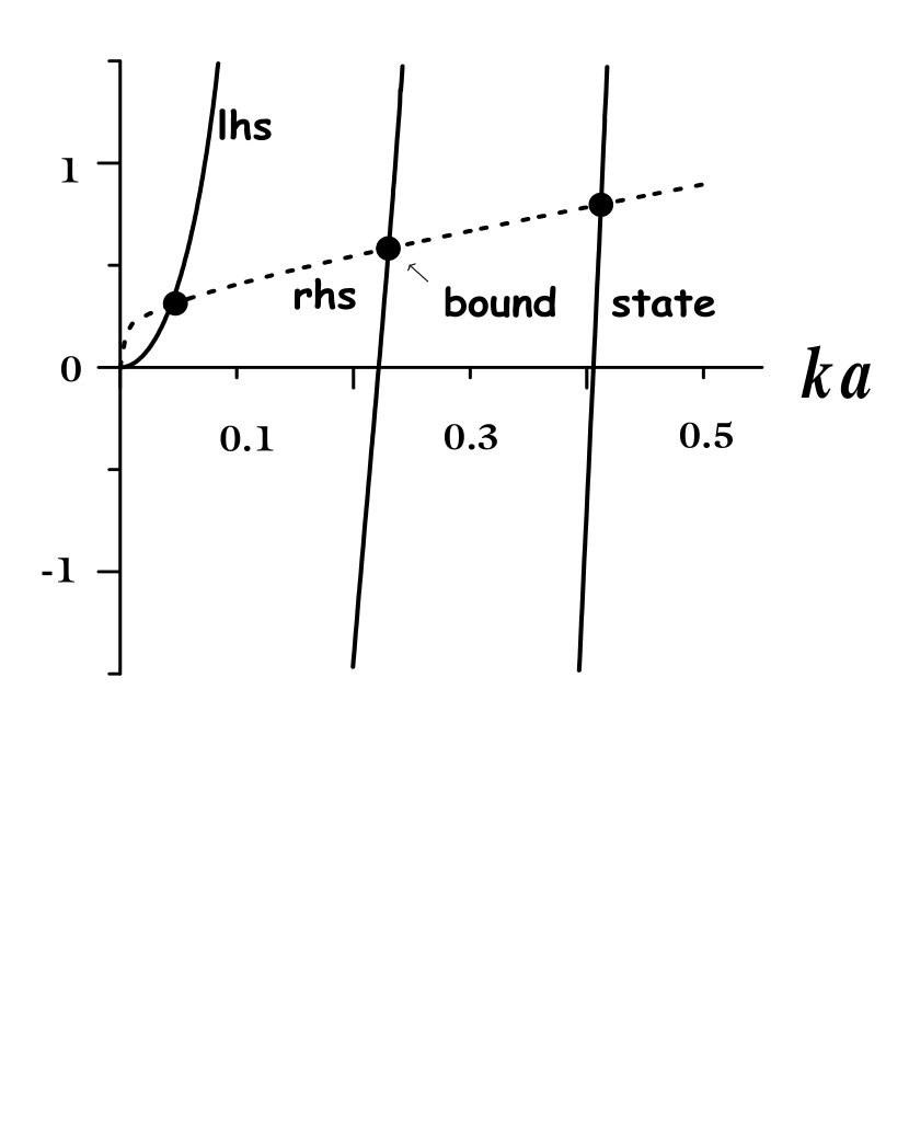
Figure 1: Rhs (dashed curve) and lhs (full curve) of (15) for the 2D well with $V_{0}/\left|E\right|=300$. Intersections of both curves marked by dots signal bound states. There is always a bound state between every two consecutive zeros of $J_{0}(x)$, or poles of the lhs of (15).

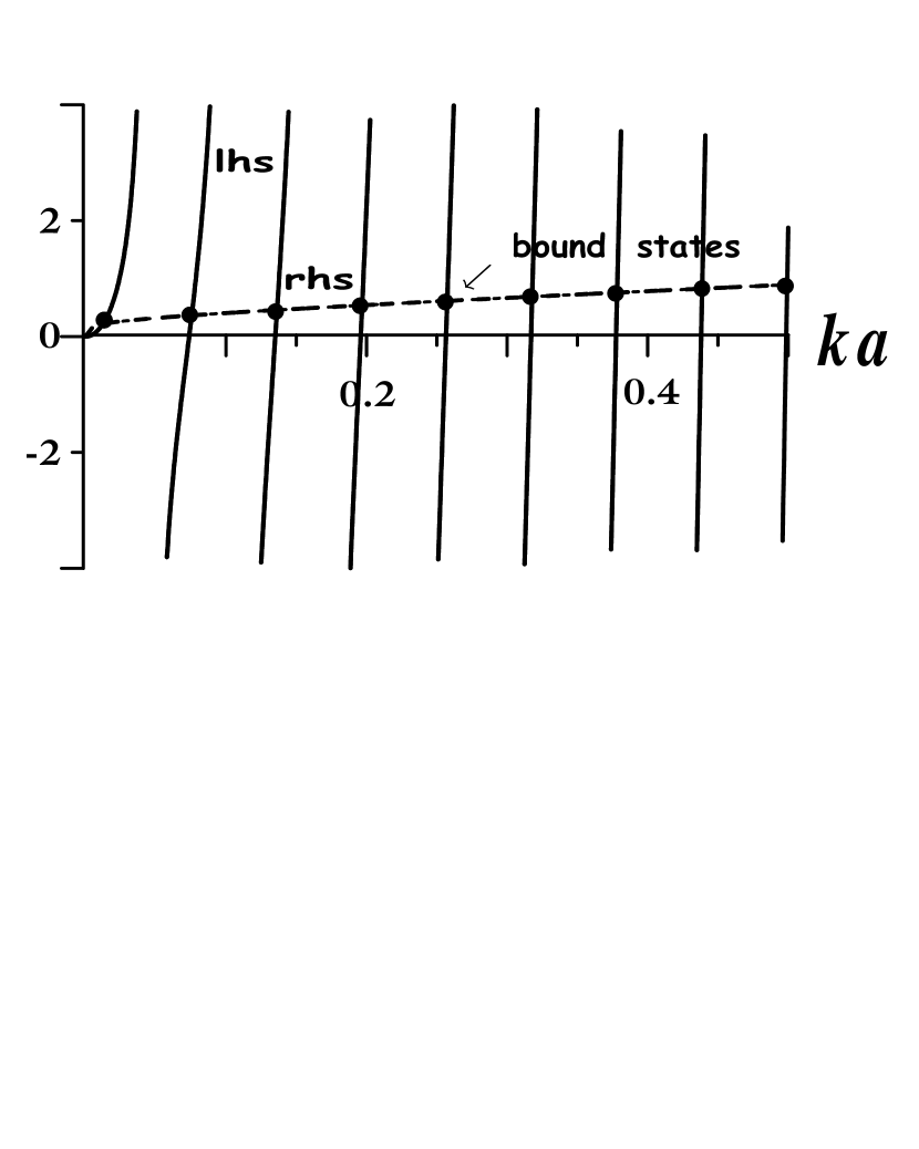
Figure 2: Same as Fig. 1 but for $V_{0}/\left|E\right|=2700$ suggesting that the number of bound states increases indefinitely as the potential well approaches the Dirac $\delta$-well limit (5).

Since $K_{1}(x)>K_{0}(x)>0$ for all $x$, the rhs of (15) is always a positive and increasing function of $ka;$ it is plotted in Fig. 1 for $V_{0}/\left|E\right|=300$ (dashed curve). As for the lhs, $J_{0}\left(x\right)$ oscillates for all $x$ so that it diverges positively whenever $J_{0}(x)=0$, then changes sign and thus drives the lhs to $-\infty$ (see full curve in figure). Clearly, there is always an intersection (bound state, marked by dots in figure) between two consecutive zeros of $J_{0}(x).$ For a given interval in $ka,$ the closer these poles are, the more bound-states there will be. Thus, for any given square well, all of the allowed bound-states lie inside an interval between ${0}$ and $k_{\max}a,$ where $k_{\max}\equiv(2mV_{0}/\hbar^{2})^{1/2}$. In such an interval the number $n$ of bound states (zeros) will be $n=$ INT($\alpha k_{\max}a/\pi$), with $\alpha\equiv\left(V_{0}/\left|E\right|-1\right)^{1/2}$ where the INT($x$) function rounds a number $x$ down to the nearest integer. Of course, the expression for $n$ is only valid after the appearance of the first pole. Then for $V_{0}/\left|E\right|=300$ as in Fig. 1, $n=3$ in the interval between $0$ and $k_{\max}a=0.5.$ In Fig. 2 are shown the bounds for $V_{0}/E=2700$ where there are $n=7$ bound states in the interval between $0$ and $k_{\max}a=0.4$ as it should be.

To construct a delta potential well $-v_{0}\delta\left({\mathbf{r}}\right)$ in 2D from the finite-ranged well (4), and through (5) ensure that $\int d^{2}{\mathbf{r}}\delta\left({\mathbf{r}}\right)=1$, requires that

$$\mathrel{\mathop{\lim}\limits_{V_{0}\rightarrow\infty,\,{}a\rightarrow 0}}V_{0}\pi a^{2}\equiv v_{0}\quad<\quad\infty.$$ (16)

Thus, as long as $\left|E\right|$ is finite $ka\equiv(\sqrt{2m\left|E\right|/\hbar^{2}})a\mathrel{\mathop{\longrightarrow}\limits_{V_{0}\rightarrow\infty,\,{}a\rightarrow 0}}0$ and we can use (Ref. [17], p. 612) $xK_{1}(x)/K_{0}(x)\mathrel{\mathop{\longrightarrow}\limits_{x\ll 1}}-1/\ln x$ for the rhs of (15). In this case the number $n$ of bound states for $\delta$-well corresponds again to the number of zeros of the lhs of (15) but in the delta limit. Here, from (16) $Ka\equiv ka\left(V_{0}/\left|E\right|-1\right)^{1/2}$ ${\smash{\mathop{\relbar\joinrel\longrightarrow}\limits_{V_{0}\rightarrow\infty,a\rightarrow 0}}}\sqrt{2mv_{0}/\pi\hbar^{2}}<\infty$ (not necessarily $\ll 1$). We will see below that the case $Ka\ll 1$ corresponds to the shallow 2D potential well of Ref. [13]. But even if $Ka$ is not $\ll 1,$ Bessel functions oscillate for large argument although their period is not constant. In this latter case (Ref. [25], p. 364) $J_{1}(x)\mathrel{\mathop{\longrightarrow}\limits_{x\gg 1}}$ $\sqrt{2/\pi x}\cos(x-3\pi/4)$ allows locating the zeros of the lhs of (15) which as $V_{0}/\left|E\right|$ is increased approach each other on the $ka$ axis, so that in the delta well limit as $V_{0}/\left|E\right|\longrightarrow\infty$ the number $n$ of bound-states increases indefinitely. Moreover, rewriting (15) as

$$\alpha x_{n}J_{1}(\alpha x_{n})K_{0}(x_{n})-x_{n}K_{1}(x_{n})J_{0}(\alpha x_{n})=0,$$ (17)

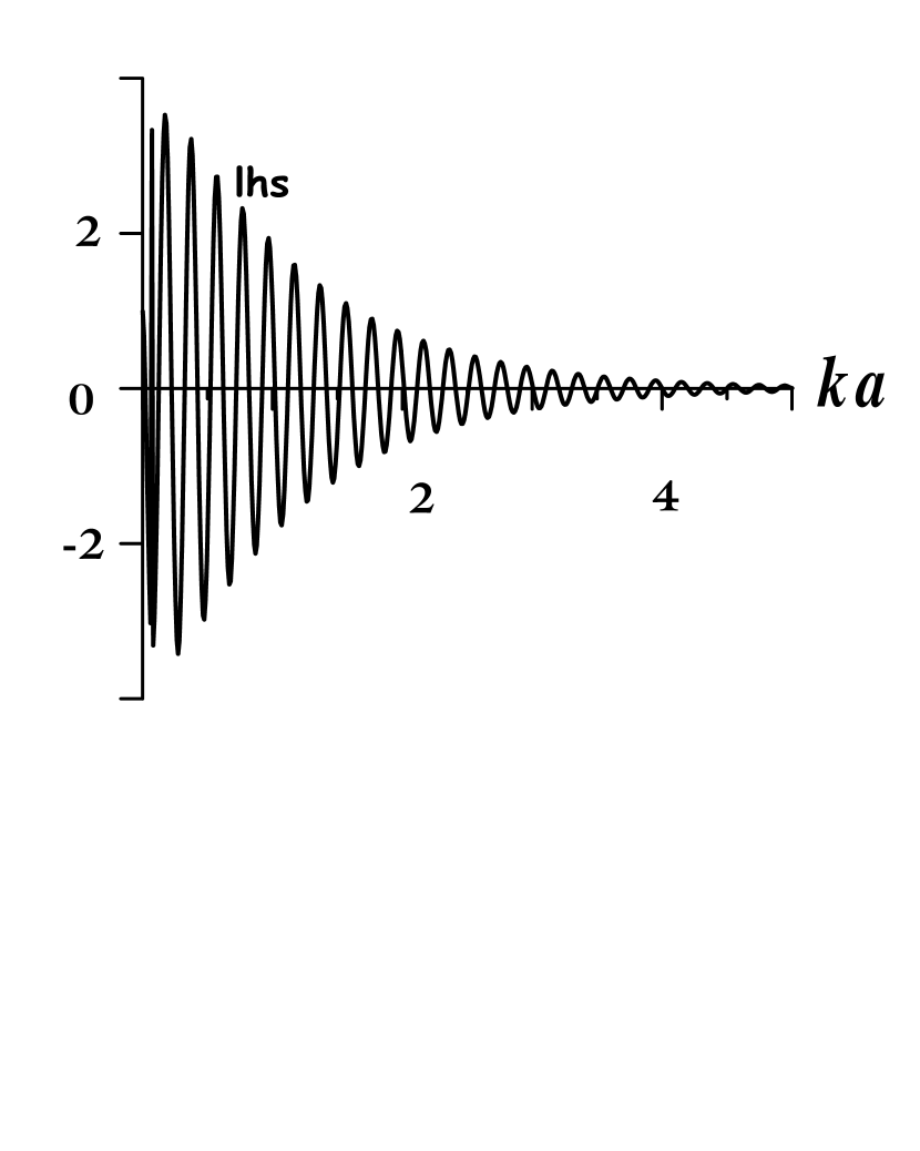
Figure 3: The bound states for the 2D $\delta$-well are associated with the zeros of the lhs of equation (17), plotted on the vertical axis. For $V_{0}/\left|E\right|=1000$, this graph illustrates the roots (bound states) of (17) which become an infinite set as we approch to the $\delta$-well limit.

bound states are easily identified from Fig. 3, where the roots of (17), say $x_{n}\equiv k_{n}a=\left(\sqrt{2m\left|E_{n}\right|/\hbar^{2}}\right)a,$ are seen to form an infinite set as $\alpha\longrightarrow\infty$. Therefore the 2D delta potential well supports an infinite number of states, for any fixed $v_{0}$, precisely as in the 3D case, this being the main conclusion of the paper. Table 1 shows the first few (numerical) $x_{n}$ roots where $E_{n}\equiv-\hbar^{2}x_{n}^{2}/2ma^{2},$ for three extreme values of $V_{0}/\left|E\right|.$

Applying the integral method of Ref. [13] for $\nu=0$ for a shallow potential well, i.e., $V_{0}\rightarrow 0$ and $\left|E\right|\ll V_{0},$ one can take both $Ka$ and $ka$ $\rightarrow 0.$ Thus, we can use $xK_{1}(x)/K_{0}(x)\mathrel{\mathop{\longrightarrow}\limits_{x\ll 1}}-1/\ln x$ in the rhs of (15), and in the lhs of (15) we note that (Ref. [25], p. 360) $J_{\nu}(x)\mathrel{\mathop{\longrightarrow}\limits_{x\ll 1}}x^{\nu}/2^{\nu}\nu!$, with $\nu=0$ and $1,$ so that $xJ_{1}(x)/J_{0}(x)\mathrel{\mathop{\longrightarrow}\limits_{x\ll 1}}$ $x^{2}/2$ . Hence we write (15) as

$$-\frac{1}{(Ka)^{2}}\simeq\frac{\ln ka}{2},$$ (18)

so that on putting $V_{0}-\left|E\right|\approx V_{0}$ (18) becomes precisely (3). In fact, for any shallow 2D circularly-symmetric potential well $V\left(r\right),$ the first bound state in Ref. [13] is given by

$$E\simeq-\frac{\hbar^{2}}{2ma^{2}}\exp\left(-\hbar^{2}/m\left|\int_{0}^{\infty}drrV(r)\right|\right),$$ (19)

which for potential (4) reduces to (3). This result in the delta limit of (16) finally becomes

$$E\simeq-\frac{\hbar^{2}}{2ma^{2}}\exp\left(-2\hbar^{2}\pi/mv_{0}\right),$$ (20)

where $v_{0}<\infty.$

IV. NEED TO REGULARIZE IN CONDENSED-MATTER SYSTEMS

Real condensed matter systems are made of many particles (bosons and/or fermions) interacting via attractive and/or repulsive forces. Attractive forces between fermions can form pairs needed for many properties such as superconductivity in solids or superfluidity in fermion liquids or trapped atomic fermion gases. However, addressing these problems with a physically realistic interaction is oftentimes difficult. As in 1D with a “bare” $\delta$-potential well, a regularized attractive $\delta$-well prevents collapse in 3D, provides the required pairs in either 2D or 3D and, of course, simplifies calculations.

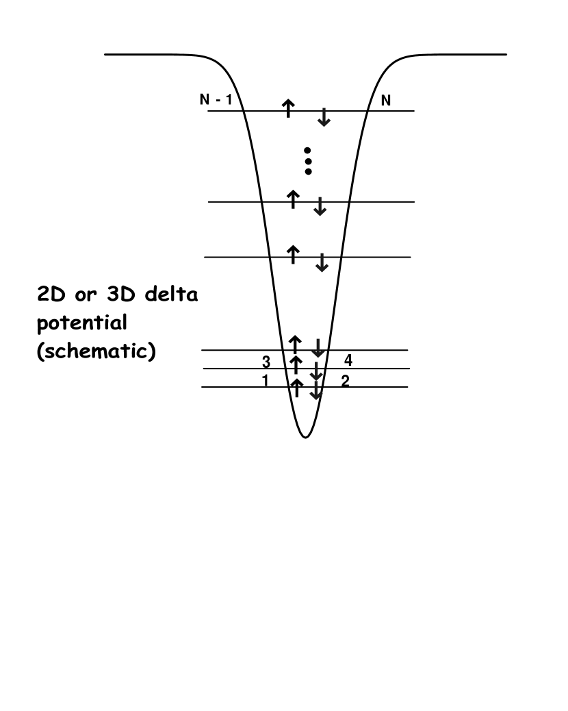
Figure 4: An $N$-fermion system with the $\delta$-well pairwise interactions produces collapse as $N\rightarrow\infty$ in 3D since both the binding energy per particle and the particle density diverge.

It is easy to imagine a trial wave function whereby, with an attractive bare $\delta$-function interfermionic interaction (i.e., before regularization), a 3D $N$-fermion system would have infinitely negative energy-per-particle (as well as infinite number-density). This is because the lowest bound level of the two-body $\delta$-well is infinitely deep in 3D, and indeed also in 2D, as was shown in the preceding sections. By the Rayleigh-Ritz variational principle the expectation energy associated with the trial wave function is a rigorous upper bound to the exact $N$-fermion ground-state energy, and hence produces collapse of the true 3D ground state of the system as $N\rightarrow\infty$. In this picture, each particle “makes its own well” but will attract to itself every other particle, two for each level, to minimize the trial expectation energy. We thus get an $N$-fermion system as schematically sketched in Fig. 4 (where the Pauli exclusion principle is explicitly being applied) that collapses as $N\rightarrow\infty.$ To avoid this unphysical collapse in 3D, and at the same time ensure pair formation in either 2D or 3D, one can “regularize” [8] the 2D and 3D finite interparticle potential wells so that in the limit the corresponding $\delta$-well possesses only one ($s$-wave) bound state. This also occurs with the Cooper/BCS model interaction [10] definable in any $d$ and with the bare $\delta$-well in 1D. The single-bound-state $\delta$-well then ensures that only pair “clusters” form, in agreement with quantized magnetic flux experiments in either elemental [26][27] or cuprate superconductors [28] in rings where the smallest flux trapped is found to be $h/2e$ (with $h$ being Planck’s constant and $e$ the electron charge). This contrasts with $h/e$ as London conjectured just on dimensional grounds, as well as with $h/ne$ ($n=3,4,...$) which is not observed in superconductors, as one would expect in vacuo in other many-particle systems with attractions that produce clusters of any size. The fact that only pair clusters occur with electrons (or “holes”) in superconductors is likely associated with clusters forming.

V. REGULARIZED 2D DELTA WELL

Regularization in either 2D or 3D starts from a finite-range square well and yields $\delta$-well with an infinitesimally small strength $v_{0}$, as we now illustrate. To be specific, we concentrate on the regularization of the 2D finite potential wells needed to mimic, in a simple way, the presence of Cooper pairs in superconductors. We thus seek a two-body square well interaction such that, in the $\delta$ limit, it possesses only one ($s$-wave) bound state. Following Ref. [8], for $d=2$ we substitute (4) by an effective two-body square-well interaction $V_{a}(r)$ which in the limit $a\rightarrow 0^{+}$ becomes $-v_{0}\delta({\mathbf{r}})$ with $v_{0}>0$, and is given by

$$V_{a}(r)=\frac{\hbar^{2}}{2m^{\ast}}\frac{2}{a^{2}\ln\left|a/a_{0}\right|}\theta(a-r),\hskip 72.26999pt(a_{0}>a>0)$$ (21)

where $m^{\ast}=m/2$ is the reduced mass of the pair, $a$ is still the well range, and $a_{0}$ is an arbitrary parameter that measures the actual strength of the interaction. Potential (21) in the delta limit (5) gives a $\delta$-well strength $v_{0}\left(a\right)\equiv-\int d^{2}rV_{a}\left(r\right)=-\pi\hbar^{2}/m^{\ast}\ln\left|a/a_{0}\right|>0$, and is thus infinitesimally small as $a\rightarrow 0^{+}$. However, this parameter can be eliminated in favor of the binding energy $B_{2}\geq 0$ of the single level, which now serves as coupling parameter. Indeed, using $v_{0}\left(a\right)$ in equation (20) for a shallow-well as in Ref. [13] but with $m^{\ast}$ instead of $m$, we obtain for the lowest energy

$$E=-\frac{\hbar^{2}}{ma_{0}^{2}}\equiv-B_{2},$$ (22)

where $0\leq B_{2}<\infty$ is the magnitude of the pair binding energy. This straightforward procedure then guarantees a simple finite-lowest-energy level well—as in 1D, see (9). Once we set the regularized two-body interaction model, result (22) can be varied as the coupling describing our superconductor model. One possibility we have now is to fix $B_{2},$ which fixes the value of $a_{0};$ the second possibility is to set $B_{2}$ by fixing the parameter $a_{0},$ which can represent the range of the wave function of the particles. One can also reduce the infinite number of bound states to only one by shifting the center of the 2D $\delta$-potential from the origin along the radial axis [29]; however the topology of this new $\delta$-potential is unsuitable to simulate real interactions between electrons.

In 3D regularization proceeds similarly [8] as in 2D except that there is no log term in (21), and instead of the binding energy (22) as coupling parameter one employs the $s$-wave scattering length which is well-defined even if, unlike 2D, the well is too shallow to support a bound state.

In an $N$-fermion system interacting pairwise via a regularized $\delta$-potential, fermions in the Fermi sea bind each other by pairs only, as required by magnetic flux quantization experiments [26][27][28], see Fig. 5. The $\delta$-potential has been used extensively in the literature [30, 31] to mimic the pair-forming interfermion interaction in, e.g., quasi-2D cuprate as well as in otherwise 3D superconductors [31, 32] and neutral-fermion superfluids [15, 16].

VI. CONCLUSIONS

A graphical proof was provided of how a 2D $\delta$-potential well supports an infinite number of bound-states as does the more familiar 3D $\delta$-potential well. Using Rayleigh-Ritz variational-principle upper-bound arguments, we then illustrated how in 3D the binding energy-per-particle of an $N$-fermion system must grow indefinitely as the number of fermions increases. In order to prevent this unphysical collapse in modeling such a system one can use regularized $\delta$-potentials in 3D as well as in 2D that by construction support a single bound state. This provides useful interfermion interaction models to study 2D and 3D condensed-matter problems. An appealing motivation for regularized $\delta$-potentials is that they fit easily within the framework of the time-independent Schrödinger equation in either coordinate or momentum space. Indeed, solving the two-body problem in the Fermi sea allows one already to exhibit Cooper pairing phenomena which is the starting point for any treatment of superconductivity or neutral-fermion superfluidity.

ACKNOWLEDGMENTS

We thank M. Fortes and O. Rojo for discussions, and acknowledge UNAM-DGAPA-PAPIIT (Mexico) grant # IN106401, and CONACyT (Mexico) grant # 27828 E, for partial support. MAS thanks Washington University, St. Louis, MO, USA, for hospitality during a sabbatical year.

$$V_{0}{\mathbf{/}}\left|E\right|$$

Table 1: First few roots $x_{n}=(\sqrt{2m\left|E_{n}\right|/\hbar^{2}})a$ of (17) for bound-states $E_{n}$ of 2D potential well according to (15), for different values of $V_{0}/\left|E\right|.$

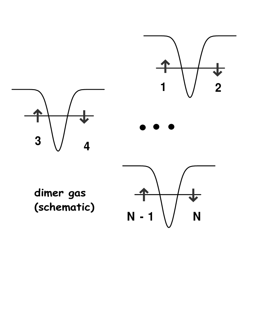
Figure 5: A dimer gas formed by single-bound-state regularized $\delta$-wells, schematically depicted. In this case, the 3D many-fermion system will not collapse since the Pauli exclusion principle prevents more than two particles from being bound in a given well.

References

- [1] G. Stan, S.M. Gatica, M. Boninsegni, S. Curtarolo, and M.W. Cole, Am. J. Phys. 67, 1170 (1999).
- [2] E. Corcoran and G. Zopette, Sci. Am. [Suppl. The Solid-State Century] (Oct. 1997) p. 25.
- [3] L.I. Glazman, Am. J. Phys. 70, 376 (2002).
- [4] F.D.M. Haldane, J. Phys. C 14, 2585 (1981).
- [5] P.W. Anderson, The theory of superconductivity in the High-Tc cuprates (Princeton University Press, NJ, 1997).
- [6] S. Albeverio, F. Gesztesy, R. Høegh-Krohn, and H. Holden, Solvable Models in Quantum Mechanics (Springer-Verlag, Berlin, 1988).
- [7] R. Jackiw, in M.A.B. Bég Memorial Volume, edited by A. Ali and P. Hoodbhoy (World Scientific, Singapore, 1991).
- [8] P. Gosdzinsky and R. Tarrach, Am. J. Phys. 59, 70 (1991).
- [9] L.N. Cooper, Phys. Rev. 104, 1189 (1956).
- [10] M. Casas, M. Fortes, M. de Llano, A. Puente, and M.A. Solís, Int. J. Theor. Phys. 34, 707 (1995).
- [11] S. Gasiorowicz, Quantum Physics (J. Wiley & Sons, NY, 1996) pp. 93-97.
- [12] D.A. Park, Introduction to the Quantum Theory (McGraw-Hill, NY, 1974), pp. 234-237.
- [13] L. Landau and E.M. Lifshitz, Quantum Mechanics (Pergamon Press, NY, 1987) pp. 162-163. A factor of 1/2 missing in this reference is included in our Eq. (3).
- [14] For a review, see M. Randeria, in: Bose-Einstein Condensation, ed. A. Griffin et al. (Cambridge University, Cambridge, 1995) p. 355.
- [15] M.J. Holland, S.J.J.M.F. Kokkelmans, M.L. Chiofalo, and R. Walser, Phys. Rev. Lett. 87 (2001) 120406.
- [16] Y. Ohashi and A. Griffin, Phys. Rev. Lett. 89 (2002) 130402.
- [17] D.L. Goodstein, States of Matter (Dover, NY, 1985) p. 386.
- [18] E.H. Lieb and M. de Llano, J. Math. Phys. 19, 860 (1978).
- [19] V.C. Aguilera-Navarro, E. Ley-Koo, M. de Llano, S.M. Peltier, and A. Plastino, J. Math. Phys. 23, 2439 (1982).
- [20] M. Casas, C. Esebbag, A. Extremera, J.M. Getino, M. de Llano, A. Plastino, and H. Rubio, Phys. Rev. A 44, 4915 (1991).
- [21] R.M. Quick , C. Esebbag and M. de Llano, Phys. Rev. B 47, 11512 (1993).
- [22] E. Merzbacher, Quantum Mechanics (J. Wiley & Sons, NY, 1998), pp. 257-263.
- [23] G. Arfken, Mathematical Methods for Physicists (Academic Press, NY, 2001).
- [24] M. de Llano, Mecánica Cuántica (Facultad de Ciencias, UNAM, 2002) 2nd Edition, p. 124.
- [25] M. Abramowitz and I.A. Stegun, Handbook of Mathematical Functions (Dover, NY, 1964).
- [26] B.S. Deaver, Jr. and W.M. Fairbank, Phys. Rev. Lett. 7, 43 (1961).
- [27] R. Doll and M. Näbauer, Phys. Rev. Lett. 7, 51 (1961).
- [28] C.E. Gough, M.S Colclough, E.M. Forgan, R.G. Jordan, M. Keene, C.M. Muirhead, I.M. Rae, N. Thomas, J.S. Abell, and S. Sutton, Nature 326, 855 (1987).
- [29] K. Chadan, N.N. Khuri, A. Martin, and Tai Tsun Wu, J. Math. Phys. 44, 406 (2003).
- [30] K. Miyake, Prog. Teor. Phys. 69, 1794 (1983).
- [31] R.M. Carter, M. Casas, J.M. Getino, M. de Llano, A. Puente, H. Rubio, and D.M. van der Walt, Phys. Rev. B. 52, 16149 (1995).
- [32] S.K. Adhikari, M. Casas, M. Fortes, M. de Llano, A. Rigo, M.A. Solís, and A.A. Valladares, Physica C 351, 341 (2001).
Tables