Damped finite-time-singularity driven by noise

Abstract

We consider the combined influence of linear damping and noise on a dynamical finite-time-singularity model for a single degree of freedom. We find that the noise effectively resolves the finite-time-singularity and replaces it by a first-passage-time or absorbing state distribution with a peak at the singularity and a long time tail. The damping introduces a characteristic cross-over time. In the early time regime the probability distribution and first-passage-time distribution show a power law behavior with scaling exponent depending on the ratio of the non linear coupling strength to the noise strength. In the late time regime the behavior is controlled by the damping. The study might be of relevance in the context of hydrodynamics on a nanometer scale, in material physics, and in biophysics.

I Introduction

The influence of noise on the behavior of nonlinear dynamical system is a recurrent theme in modern statistical physics Freidlin and Wentzel (1998). In a particular class of systems the nonlinear character gives rise to finite-time-singularities, that is solutions which cease to be valid beyond a particular finite time span. One encounters finite-time-singularities in stellar structure, turbulent flow, and bacterial growth Kerr and Brandenburg (1999); Brenner et al. (1997, 1998). The phenomenon is also seen in Euler flows and in free-surface-flows Cohen et al. (1999); Eggers (1997). Finally, finite-time-singularities are encountered in modelling in econophysics, geophysics, and material physics Sornette and Andersen (2002); Ide and Sornette (2001); Sornette and Helmstetter (2002); Gluzman et al. (2001); Johansen and Sornette (2002).

In the context of hydrodynamical flow on a nanoscale Eggers (2002), where microscopic degrees of freedom come into play, it is a relevant issue how noise influences the hydrodynamical behavior near a finite-time-singularity. Leaving aside the issue of the detailed reduction of the hydrodynamical equations to a nanoscale and the influence of noise on this scale to further study, we assume in the present context that a single variable or “reaction coordinate” effectively captures the interplay between the singularity and the noise.

In a recent paper Fogedby and Poukaradze (2002) we investigated a simple generic model system with one degree of freedom governed by a nonlinear Langevin equation driven by Gaussian white noise,

$$\frac{dx}{dt}=-\frac{\lambda}{2|x|^{1+\mu}}+\eta~{},~{}~{}~{}\langle\eta\eta\rangle(t)=\Delta\delta(t).$$ (1)

The model is characterized by the coupling parameter $\lambda$, determining the amplitude of the singular term, the index $\mu\geq 0$, characterizing the nature of the singularity, and the noise parameter $\Delta$, determining the strength of the noise correlations. Specifically, in the case of a thermal environment at temperature $T$ the noise strength $\Delta\propto T$.

In the absence of noise this model exhibits a finite-time-singularity at a time $t_{0}$, where the variable $x$ vanishes with a power law behavior determined by $\mu$. When noise is added the finite-time-singularity event at $t_{0}$ becomes a statistical event and is conveniently characterized by a first-passage-time distribution $W(t)$ Redner (2001). For vanishing noise we have $W(t)=\delta(t-t_{0})$, restating the presence of the finite-time-singularity. In the presence of noise $W(t)$ develops a peak about $t=t_{0}$, vanishes at short times, and acquires a long time tail.

The model in Eq. (1) has also been studied in the context of persistence distributions related to the nonequilibrium critical dynamics of the two-dimensional XY model Bray (2000) and in the context of non-Gaussian Markov processes Farago (2000). Finally, regularized for small $x$, the model enters in connection with an analysis of long-range correlated stationary processes Lillo et al. (2002).

From our analysis in ref. Fogedby and Poukaradze (2002) it followed that for $\mu=0$, the logarithmic case, the distribution at long times is given by the power law behavior

$$W(t)\sim t^{-\alpha}~{}~{},~{}~{}~{}\alpha=\frac{3}{2}+\frac{\lambda}{2\Delta}.$$ (2)

For vanishing nonlinearity, i.e., $\lambda=0$, the finite-time-singularity is absent and the Langevin equation (1) describes a simple random walk of the reaction coordinate, yielding the well-known exponent $\alpha=3/2$ Redner (2001); Stratonovich (1963); Risken (1989). In the nonlinear case with a finite-time-singularity the exponent attains a non-universal correction, depending on the ratio of the nonlinear strength to the strength of the noise; for a thermal environment the correction is proportional to $1/T$. In the generic case for $\mu>0$ we found that the fall-off is slower and that the correction to the random walk result is given by a stretched exponential

$$W(t)\sim t^{-3/2}\exp[-A(t^{-\mu/(2+\mu)}-1)],$$ (3)

where $A\rightarrow\lambda/\Delta\mu$ for $\mu\rightarrow 0$.

In our studies so far we have ignored damping. It is, however, clear that in realistic physical situations friction or damping must enter on the same footing as the noise. This follows from the Einstein relation or more generally from the fluctuation-dissipation theorem relating the damping to the noise. In the present paper we attempt to amend this situation and thus proceed to extend the analysis in ref. Fogedby and Poukaradze (2002) to the case of linear damping. We shall here only consider the logarithmic case for $\mu=0$.

For this purpose we consider the following model for one degree of freedom:

$$\frac{dx}{dt}=-\gamma x-\frac{\lambda}{2|x|}+\eta~{},~{}~{}~{}\langle\eta\eta\rangle=\Delta\delta(t).$$ (4)

In addition to the coupling parameter $\lambda$, and the noise parameter $\Delta$, this model is also characterized by the damping constant $\gamma$. Assuming for convenience a dimensionless variable $x$ the coupling and the noise strengths $\lambda$ and $\Delta$ have the dimension $1/\text{time}$. The ratios $\lambda/\Delta$ and $\gamma/\Delta$ are thus dimensionless parameters characterizing the behavior of the system.

It follows from our analysis below that the damping constant sets an inverse time scale $1/\gamma$. At intermediate time scales for $\gamma t\ll 1$ the distribution exhibits the same power law behavior as in the undamped case given by Eq. (2). At long times for $\gamma t\gg 1$ the distribution falls off exponentially with time constant $1/\gamma(1+\lambda/\Delta)$, i.e.,

$$W(t)\propto\exp[-\gamma(1+\lambda/\Delta)t].$$ (5)

The paper is organized in the following manner. In Section II we introduce the finite-time-singularity model with linear damping and discuss its properties. In Section III we review the weak noise WKB phase space approach to the Fokker-Planck equation, apply it to the finite-time-singularity problem with damping, discuss the associated dynamical phase space problem and the long time properties of the distributions. In Section IV we derive an exact solution of the Fokker-Planck equation and present an expression for the first-passage-time distribution. In Section V we present a summary and a conclusion. In the present treatment we draw heavily on the analysis in ref. Fogedby and Poukaradze (2002). In Appendix A aspects of the exact solution are discussed in more detail; in Appendix B we consider the weak noise limit of the exact solution.

II Model

In terms of a free energy or potential $F$ we can express Eq. (4) in the form

$$\frac{dx}{dt}=-\frac{1}{2}\frac{dF}{dx}+\eta(t),$$ (6)

where $F$ has the form

$$F=\gamma x^{2}+\lambda\ln|x|.$$ (7)

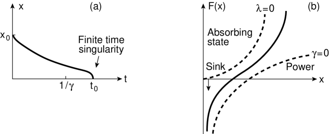
Figure 1: In a) we show the time evolution of the single degree of freedom $x$. At times shorter than the cross-over time $1/\gamma$ the variable $x$ falls off exponentially. At times beyond $1/\gamma$ the variable $x$ reaches the absorbing state $x=0$ at a finite time $t_{0}$. In b) we depict the free energy $F(x)$ driving the equation. For $\lambda=0$ the free energy forms a confining harmonic well, for $\gamma=0$ we have the absorbing state case discussed in ref. Fogedby and Poukaradze (2002). In the general case the absorbing state $x=0$ corresponds to the sink in $F(x)$.

The free energy has a logarithmic sink and drives $x$ to the absorbing state $x=0$. For large $x$ the free energy has the form of a harmonic well potential confining the motion. In Fig. 1 we have depicted the free energy in the various cases.

II.1 The noiseless case

In the case of vanishing noise Eq. (6) is readily solved. We obtain

$$x(t)=\left[\frac{\lambda}{2\gamma}\right]^{1/2}\left[e^{2\gamma(t_{0}-t)}-1\right]^{1/2},$$ (8)

with a finite-time-singularity at

$$t_{0}=\frac{1}{2\gamma}\log\left|1+\frac{2\gamma}{\lambda}x_{0}^{2}\right|.$$ (9)

The initial value of $x$ is $x_{0}$ at time $t=0$. In the presence of damping $x$ initially falls off exponentially due to the confining harmonic potential with a time constant $1/\gamma$. For times beyond $1/\gamma$ the nonlinear term takes over and drives $x$ to zero at time $t_{0}$, i.e., $x$ falls into the sink in $F$. In Fig. 1 we have shown the noiseless solution $x(t)$.

II.2 The noisy case

Summarizing the discussion in ref. Fogedby and Poukaradze (2002), the stochastic aspects of the finite-time-singularity in the presence of noise are analyzed by focusing on the time dependent probability distribution $P(x,t)$ and the derived first-passage-time or absorbing state probability distribution $W(t)$. The distribution $P(x,t)$ is defined according to van Kampen (1992); Risken (1989) $P(y,t)=\langle\delta(y-x(t))\rangle$ where $x$ is a stochastic solution of Eq. (6) and $\langle\cdots\rangle$ indicates an average over the noise $\eta$ driving $x$. In the absence of noise $P(y,t)=\delta(y-x(t))$, where $x$ is the deterministic solution given by Eq. (8) and depicted in Fig 1. At time $t=0$ the variable $x$ evolves from the initial condition $x_{0}$, implying the boundary condition $P(x,0)=\delta(x-x_{0})$.

At short times $x$ is close to $x_{0}$ and the singular term and the damping term are not yet operational. In this regime we obtain ordinary random walk with the Gaussian distribution, $P(x,t)=(2\pi\Delta t)^{-1/2}\exp\left[-(x-x_{0})^{2}/2\Delta t\right]$. At a time scale given by $1/\gamma$ the damping drives $x$ towards a stationary distribution given by $P\propto\exp({-F/\Delta)}$. However, at longer times beyond the scale $1/\gamma$, the barrier $\lambda/2x$ comes into play preventing $x$ from crossing the absorbing state $x=0$. This is, however, a random event which can occur at an arbitrary time instant, i.e., the finite-time-singularity at $t_{0}$ in the deterministic case is effectively resolved in the noisy case. For not too large noise strength the distribution is peaked about the noiseless solution and vanishes for $x\rightarrow 0$, corresponding to the absorbing state, implying the boundary condition

$$P(0,t)=0~{}.$$ (10)

In order to model a possible experimental situation the first-passage-time or absorbing state distribution $W(t)$ is of more direct interest van Kampen (1992); Gardiner (1997).

Since $P(0,t)=0$ for all $t$ due to the absorbing state, the probability that $x$ is not reaching $x=0$ in time $t$ is thus given by $\int_{0}^{\infty}P(x,t)dx$, implying that the probability $-dW$ that $x$ does reach $x=0$ in time $t$ is $-dW=-\int_{0}^{\infty}dxdt(dP/dt)$, yielding the absorbing state distribution $W(t)=-\int_{0}^{\infty}dx~{}\partial P(x,t)/\partial t$ Risken (1989). In the absence of noise $P(x,t)=\delta(x-x(t))$ and $W(t)=\delta(t-t_{0})$, in accordance with the finite time singularity at $t=t_{0}$. For weak noise $W(t)$ peaks about $t_{0}$ with vanishing tails for small $t$ and large $t$.

The distribution $P(x,t)$ satisfies the Fokker-Planck equation van Kampen (1992); Gardiner (1997)

$$\frac{\partial P}{\partial t}=\frac{1}{2}\frac{\partial}{\partial x}\left[\frac{dF}{dx}P+\Delta\frac{\partial P}{\partial x}\right]~{},$$ (11)

in the present case subject to the boundary conditions $P(x,0)=\delta(x-x_{0})$ and $P(0,t)=0$. The Fokker-Planck equation has the form of a conservation law $\partial P/\partial t+\partial J/\partial x=0$, defining the probability current $J=(1/2)(dF/dx)P-(1/2)\Delta\partial P/\partial x$ and we obtain for $W(t)$ the expression

$$W(t)=\frac{1}{2}\left[\frac{dF}{dx}P+\Delta\frac{\partial P}{\partial x}\right]_{x=0},$$ (12)

to be used in our further analysis. Note that there is a sign error in Eq. (3.8) in ref. Fogedby and Poukaradze (2002).

III Weak noise approach

In this section we apply a weak noise canonical phase space approach to the damped finite-time-singularity model and infer the general long time behavior. The treatment follows closely the analysis in ref. Fogedby and Poukaradze (2002).

III.1 The phase space method

From a structural point of view the Fokker-Planck equation (11) has the form of an imaginary-time Schrödinger equation $\Delta\partial P/\partial t=HP$, driven by the Hamiltonian or Liouvillian $H$. The noise strength $\Delta$ plays the role of an effective Planck constant and $P$ corresponds to the wavefunction. Drawing on this parallel we have in recent work in the context of the Kardar-Parisi-Zhang equation for a growing interface elaborated on a weak noise nonperturbative WKB phase space approach to a generic Fokker-Planck equation for extended system Fogedby (1999a, b); Fogedby and Brandenburg (2002). In the case of a single degree of freedom this method amounts to the eikonal approximation Risken (1989); Roy (1993); Gardiner (1997), see also Graham (1973, 1989). For systems with many degrees of freedom the method has for example been expounded in Falkovich et al. (1996), based on the functional formulation of the Langevin equation Martin et al. (1973); Janssen (1976). In the present formulation Fogedby (1999a, b); Fogedby and Brandenburg (2002) the emphasis is on the canonical phase space analysis and the use of dynamical system theory Strogatz (1994); Ott (1993).

The weak noise WKB approximation corresponds to the ansatz $P\propto\exp[-S/\Delta]$. The weight function or action $S$ then to leading asymptotic order in $\Delta$ satisfies a Hamilton-Jacobi equation $\partial S/\partial t+H=0$ which in turn implies a principle of least action and Hamiltonian equations of motion Landau and Lifshitz (1959); Goldstein (1980). In the present context the Hamiltonian takes the form

$$H=\frac{1}{2}p(p-\frac{\lambda}{x}-2\gamma x),$$ (13)

yielding the Hamilton equations of motion

$$\frac{dx}{dt}=-\gamma x-\frac{\lambda}{2x}+p,$$ (14)

$$\frac{dp}{dt}=\gamma p-\frac{1}{2}\frac{\lambda}{x^{2}}p.$$ (15)

These equations replace the Langevin equation (4) with the noise $\eta$ represented by the momentum $p=\partial S/\partial x$, conjugate to $x$. The equations (14) and (15) determine orbits in a canonical phase space spanned by $x$ and $p$. Since the system is conserved the orbits lie on the constant energy manifold(s) given by $E=H$. The action associated with an orbit from $x_{0}$ to $x$ in time $t$ has the form

$$S(x_{0}\rightarrow x,t)=\int_{0}^{t}dt\left[p\frac{dx}{dt}-H\right].$$ (16)

According to the ansatz the probability distribution is then given by

$$P(x,t)=P(x_{0}\rightarrow x,t)\propto\exp\left[-\frac{S(x_{0}\rightarrow x,t)}{\Delta}\right]~{}.$$ (17)

III.2 Long time orbits

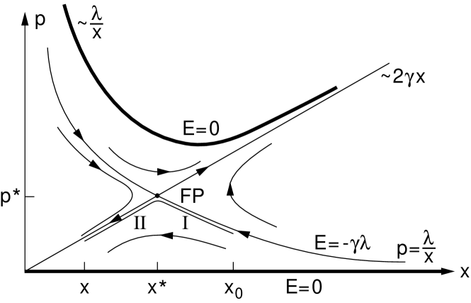
Figure 2: We show the topology of phase space. The bold lines indicate the zero energy sub-manifolds. The invariant heteroclinic orbits $p=2\gamma x$ and $p=\lambda/x$ passing through the saddle point FP at $(x^{\ast},p^{\ast})=[(\lambda/2\gamma)~{}{1/2},(2\gamma\lambda)^{1/2}]$ have energy $-\gamma\lambda$. The arrows indicate the direction of the flow. The long time orbit from $x_{0}$ to $x$ passes close to the fixed point. The part of the orbit following the invariant manifold $p=\lambda/x$ and entering in our long time estimate is denoted I; the part of the orbit close to the $p=2\gamma x$ manifold is denoted II.

The zero-energy manifolds delimiting the phase space orbits follow from Eq. (13) and are given $p=0$ and $p=2\gamma x+\lambda/2x$. The $p=0$ sub-manifold corresponds to the noiseless or deterministic case discussed above. The $p=\lambda/x+2\gamma x$ sub-manifold corresponds to the noisy case. By insertion in Eq. (15) we obtain $dx/dt=\gamma x+\lambda/2x$, i.e., the motion on the noisy sub-manifold is time reversed of the motion on the noiseless sub-manifold. The orbit structure in phase space is moreover controlled by the hyperbolic fixed point at $(x^{\ast},p^{\ast})=[(\lambda/2\gamma)^{1/2},(2\gamma\lambda)^{1/2}]$. The heteroclinic orbits passing through the fixed point are given by $p=\lambda/x$ and $p=2\gamma x$ and the energy of the invariant manifold is $E^{\ast}=-\gamma\lambda$. In Fig 2 we have depicted the phase space with the zero-energy manifolds, the fixed point, the heteroclinic orbits and some characteristic orbits.

The long time behavior of the distribution is determined by an orbit from $x_{0}$ to $x$ traversed in time $t$. In the long time limit this orbit must pass close to the hyperbolic fixed point. Note that in the limit $\gamma\rightarrow 0$ the fixed point migrates to infinity in the $x$ direction and the long time orbits approach the zero energy sub-manifolds which thus determine the asymptotic properties as discussed in ref. Fogedby and Poukaradze (2002).

Independent of whether the initial value $x_{0}$ is greater or smaller than the fixed point value $x^{\ast}$, the long time orbit follows the invariant $p=\lambda/x$ manifold towards the fixed point. At the fixed point the orbit slows down and then speeds up again as the orbit follows the other invariant manifold $p=2\gamma x$ towards the endpoint $x$ reached in time $t$. This behavior is also depicted in Fig 2.

This scenario allows a simple analysis of the long time behavior of the distribution $P(x,t)$ and the first-passage-distribution $W(t)$. Close to the invariant manifolds with energy $E^{\ast}=-\gamma\lambda$ the action associated with an orbit from $x_{0}$ to $x$ follows from Eq. (16) and is given by

$$S=-E^{\ast}t+\int_{x_{0}}^{x^{\ast}}dx\frac{\lambda}{x}+\int_{x^{\ast}}^{x}dx2\gamma x,$$ (18)

or, denoting the relevant manifolds by a subscripts, see Fig. 2,

$$S=\lambda\gamma t+\lambda\log\left|\frac{x^{\ast}}{x_{0}}\right|_{\text{I}}+\gamma(x^{2}-x^{\ast 2})_{\text{II}}.$$ (19)

At long times we only have to consider the contribution from the orbit leading up to the fixed point. Inserting the manifold condition $p=\lambda/x$ in the equation of motion (14) we thus obtain $dx/dt=-\gamma x+\lambda/2x$ with solution

$$x(t)^{2}=x_{0}^{2}e^{-2\gamma t}+x^{\ast 2}(1-e^{-2\gamma t}).$$ (20)

III.3 Discussion

It follows from Eq. (20) that the damping $\gamma$ sets an inverse time scale delimiting two kinds of characteristic behavior. First, for $t\rightarrow\infty$ the orbit approaches the fixed point $x^{\ast}$. For $\gamma t\gg 1$ we have $x^{2}=x^{\ast 2}(1-\exp(-2\gamma t))$ and $x$ approaches the fixed point in an exponential fashion. On the other hand, in the intermediate time region for $\gamma t\ll 1$ and for $\gamma t\gg x_{0}^{2}$ and $\lambda t\gg x_{0}^{2}$ we obtain $x^{2}=x_{0}^{2}+2t\gamma x^{\ast}=x_{0}^{2}+\lambda t\sim\lambda t$.

By insertion in the expression (19) for the action we then obtain in the late time regime for $\gamma t\gg 1$

$$S(t)\sim\lambda\gamma t-\frac{\lambda}{2}e^{-2\gamma t},$$ (21)

yielding the distribution and ensuing first-passage-time distribution

$$P(t)\propto W(t)\propto\exp(-\lambda\gamma t/\Delta).$$ (22)

Likewise, we have in the intermediate time regime $\gamma t\ll 1$

$$S(t)\sim\lambda\gamma t+\frac{\lambda}{2}\log|t|,$$ (23)

giving rise to the distribution and first-passage-time distribution

$$P(t)\propto W(t)\propto|t|^{-\frac{\lambda}{2\Delta}}.$$ (24)

These results hold in the weak noise limit. We note that at long times $W(t)$ falls of exponentially with a time constant given by $\Delta/\lambda\gamma$. In the intermediate time regime $W(t)$ exhibits a power law behavior with exponent $-\lambda/2\Delta$, independent of $1/\gamma$ defining the cross-over time. These results will also be recovered from the exact solution discussed in the next sections.

IV Exact solution

In this section we return to the Fokker-Planck equation (11) and present an exact solution. This solution is an extension of the solution presented in ref. Fogedby and Poukaradze (2002) and the analysis proceeds in much the same way. Details are discussed in Appendices A and B.

IV.1 Quantum particle in a harmonic potential with centrifugal barrier

The Fokker Planck equation has the form

$$\frac{\partial P}{\partial t}=\frac{\Delta}{2}\frac{\partial^{2}P}{\partial x^{2}}+\left(\gamma x+\frac{\lambda}{2x}\right)\frac{\partial P}{\partial x}+\left(\gamma-\frac{\lambda}{2x^{2}}\right)P.$$ (25)

Eliminating the first order term by means of the gauge transformation

$$\exp(h)=|x|^{-\lambda/2\Delta}e^{-\gamma x^{2}/2\Delta},$$ (26)

we can express the equation in the form

$$-\Delta\frac{\partial}{\partial t}\left[\exp(-h)P\right]=H\left[\exp(-h)P\right],$$ (27)

where the Hamiltonian $H$ driving $P$ is given by

$$H=-\frac{1}{2}\Delta^{2}\frac{\partial^{2}}{\partial x^{2}}+\frac{\lambda^{2}}{8}\left[1+\frac{2\Delta}{\lambda}\right]\frac{1}{x^{2}}+\frac{\Delta\gamma}{2}\left(\frac{\lambda}{\Delta}-1\right)+\frac{\gamma^{2}}{2}x^{2}.$$ (28)

This Hamiltonian describes the motion of a unit mass quantum particle in one dimension in a harmonic potential subject to a centrifugal barrier of strength $(\lambda^{2}/8)(1+2\Delta/\lambda)$ at the origin; $\Delta$ plays the role of an effective Planck constant. Note that in Eq. (6.4) in ref. Fogedby and Poukaradze (2002) the factor $\Delta/2$ should read $1/\Delta$.

For $\lambda=0$ and $\gamma=0$ both the barrier and the confining potential are absent; the spectrum of $H$ forms a band and the particle can move over the whole axis. This case corresponds to ordinary random walk Risken (1989). Incorporating the absorbing state condition in Eq. (10) by means of the method of mirrors we obtain the results presented in ref. Fogedby and Poukaradze (2002), i.e.,

$$P(x,t)=(2\pi\Delta t)^{-1/2}\left[\exp\left[-\frac{(x-x_{0})^{2}}{2\Delta t}\right]-\exp\left[-\frac{(x+x_{0})^{2}}{2\Delta t}\right]\right],$$ (29)

in the half space $x\geq 0$, and for the absorbing state distribution

$$W(t)=\left(\frac{2}{\pi}\right)^{1/2}x_{0}\exp(-x_{0}^{2}/2\Delta t)(\Delta t)^{-3/2}.$$ (30)

For $\lambda\neq 0$ and $\gamma=0$ the particle cannot cross the barrier and is confined to either half space; this corresponds to the case of a finite-time-singularity subject to noise and an absorbing state at $x=0$ and was discussed in detail in ref. Fogedby and Poukaradze (2002); for reference we give the obtained results below. Note that $x$ and $x_{0}$ should be interchanged in Eq. (6.5) and that a factor $\Delta$ is missing in Eq. (6.6) in ref. Fogedby and Poukaradze (2002).

$$P(x,t) =\frac{x_{0}^{\lambda/2\Delta+1/2}}{x^{\lambda/2\Delta-1/2}}\frac{\exp\left(-\frac{x^{2}+x_{0}^{2}}{2\Delta t}\right)}{\Delta t}I_{\frac{1}{2}+\frac{\lambda}{2\Delta}}\left(\frac{xx_{0}}{\Delta t}\right).$$ (31)

$$W(t) =\frac{2\Delta x_{0}^{1+\lambda/\Delta}}{\Gamma(1/2+\lambda/2\Delta)}\exp(-x_{0}^{2}/2\Delta t)(2\Delta t)^{-\frac{3}{2}-\frac{\lambda}{2\Delta}}~{}.$$ (32)

In the present case for $\lambda\neq 0$ and $\gamma\neq 0$ the problem corresponds to the motion of a particle in a harmonic potential with a centrifugal barrier at $x=0$. The spectrum is discrete and becomes continuous for $\gamma=0$. The problem is readily analyzed in terms of confluent hypergeometric functions, more specifically Laguerre polynomials Lebedev (1972); Gradshteyn and Ryzhik (1965). Incorporating the initial condition $P(x,0)=\delta(x-x_{0})$ and introducing the time scaled variables

$$x=\tilde{x}\exp(-\gamma t/2),$$ (33)

$$x_{0}=\tilde{x}_{0}\exp(+\gamma t/2),$$ (34)

we find for $P(x,t)$

$$P(x,t)=\frac{\tilde{x}_{0}^{\lambda/2\Delta+1/2}}{\tilde{x}^{\lambda/2\Delta-1/2}}\frac{\gamma e^{\gamma t/2}}{\Delta\sinh{\gamma t}}\exp\left[-\frac{\gamma(\tilde{x}^{2}+\tilde{x}_{0}^{2})}{2\Delta\sinh{\gamma t}}\right]I_{\frac{1}{2}+\frac{\lambda}{2\Delta}}\left(\frac{\gamma}{\Delta}\frac{\tilde{x}\tilde{x}_{0}}{\sinh\gamma t}\right),$$ (35)

and correspondingly for the absorbing state distribution

$$W(t)=\frac{2\Delta\tilde{x}_{0}^{1+\lambda/\Delta}}{\Gamma(1/2+\lambda/2\Delta)}\exp\left[{-\frac{\gamma\tilde{x}_{0}^{2}}{2\Delta\sinh{\gamma t}}}\right]\exp(\gamma t)\left(\frac{\gamma}{2\Delta\sinh\gamma t}\right)^{\frac{3}{2}+\frac{\lambda}{2\Delta}}.$$ (36)

In Eqs. (31) and (35) $I_{\nu}$ is the Bessel function of imaginary argument, $I_{\nu}(z)=(-i)^{\nu}J_{\nu}(iz)$ Mathews and Walker (1973).

V Discussion and conclusion

Focussing on the expression (36) for the first-passage-time distribution $W(t)$ we note that the damping constant $\gamma$ defines two distinct time regimes, $1/\gamma$ setting the characteristic cross-over time. In the long time limit for $\gamma t\gg 1$ the damping constant controls the behavior of $W(t)$. From Eq. (36) we infer

$$W(t)\propto\frac{2\Delta x_{0}^{1+\lambda/\Delta}}{\Gamma(1/2+\lambda/2\Delta)}\left(\frac{\gamma}{\Delta}\right)^{3/2+\lambda/2\Delta}\exp[-\gamma(1+\lambda/\Delta)t],$$ (37)

i.e., $W(t)$ falls off exponentially with an effective damping constant $\gamma(1+\lambda/\Delta)$ renormalized by the ratio $\lambda/\Delta$ of the nonlinear strength to the noise strength. We note that for $\Delta\rightarrow 0$ the result is in accordance with the weak noise phase space derivation in Sec. III. In the intermediate time regime for $\gamma t\ll 1$ the damping constant $\gamma$ drops out and we obtain

$$W(t)\propto\frac{2\Delta x_{0}^{1+\lambda/\Delta}}{\Gamma(1/2+\lambda/2\Delta)}\exp(-x_{0}^{2}/2\Delta t)\left(\frac{1}{2\Delta t}\right)^{3/2+\lambda/2\Delta}.$$ (38)

For $2\Delta t\gg x_{0}^{2}$ the distribution $W(t)$ exhibits a power law behavior with the same exponent $3/2+\lambda/2\Delta$ as in the undamped case for $\gamma=0$. For weak noise this result is again in agreement with the estimate in Sec. III.

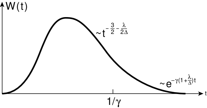
Figure 3: We sketch the first-passage-time distribution $W(t)$ as a function of $t$. In the limit $\rightarrow t0$ $W(t)$ vanishes exponentially; about the finite-time-singularity $W(t)$ exhibits a maximum. At intermediate times for $\gamma t\ll 1$ the distribution exhibits a power law behavior with scaling exponent $3/2+\lambda/2\Delta$. In the long time limit for $\gamma t\gg 1$ an exponential fall-off with time constant $\gamma(1+\lambda/\Delta)$ characterizes the behavior of $W(t)$

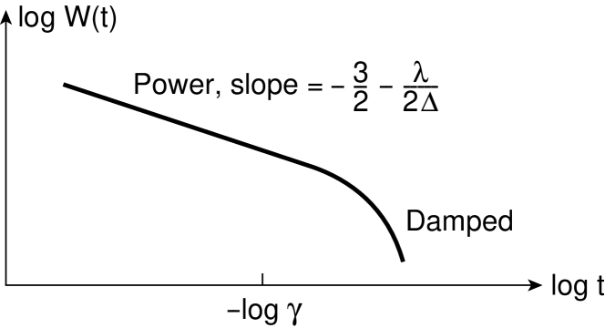
Figure 4: In this figure we sketch the behavior of $W(t)$ in a log-log plot. At intermediate times earlier that $1/\gamma$ we have scaling behavior with exponent $3/2+\lambda/2\Delta$, corresponding to a constant negative slope. In the long time limit the curve dips down indicating the cross-over to exponential behavior.

In the short time limit $W(t)$ vanishes exponentially and shows a maximum about the finite-time-singularity. In Fig. 3 we have depicted the first-passage-time-distribution as a function of t. In Fig. 4 we illustrate the behavior of $W(t)$ in a log-log representation.

In this paper we have extended the model discussed in ref. Fogedby and Poukaradze (2002) to include a linear damping term. Not surprisingly, the damping changes the long time behavior of the physically relevant first-passage-time distribution. The finite-time-singularity occurring at time $t_{0}$ in the noiseless case is still effectively resolved by the noise, becoming a random event, but the power law scaling behavior with scaling exponent $\alpha=3/2+\lambda/2\Delta$ is limited to early times compared with the cross-over time $1/\gamma$ set by the damping constant. In the long time limit beyond $1/\gamma$ the damping gives rise to an exponential fall-off and the scaling property ceases to be valid. To the extent that the present simple model might apply to physical phenomena where damping is always present, we must conclude that an eventual power law scaling presumably is confined to a time window determined by the size of the damping.

Appendix A Exact solution of the Fokker-Planck equation

In this appendix we discuss the exact solution of the Fokker-Planck equation in more detail. Denoting the normalized eigenfunction of $H$ in Eq. (28) and the associated eigenvalues by $\Psi_{n}$ and $\Delta^{2}E_{n}/2$, respectively, we obtain, incorporating the initial condition $P(x,0)=\delta(x-x_{0})$ and the gauge transformation, the following expression for the distribution

$$P(x,t)=\sum_{n}e^{-\Delta E_{n}t/2}e^{-\gamma(x^{2}-x_{0}^{2})/2\Delta}(x/x_{0})^{-\lambda/2\Delta}\Psi_{n}(x)\Psi_{n}^{\ast}(x_{0}).$$ (39)

By means of the transformation $\Psi(x)=x^{1+\lambda/2\Delta}\exp{-\gamma x^{2}/2\Delta}G(\gamma x^{2}/\Delta)$ it follows that $G$ is a solution of the degenerate hypergeometric equation Lebedev (1972); Gradshteyn and Ryzhik (1965). For the discrete spectrum we choose the polynomial form and further analysis shows that the eigenfunctions $\Psi_{n}$ are given in terms of the Laguerre polynomials $L_{n}^{\alpha}$ Lebedev (1972); Gradshteyn and Ryzhik (1965). For the normalized eigenfunctions we thus obtain

$$\Psi_{n}=\left[2\left(\frac{\gamma}{\Delta}\right)^{3/2+\lambda/2\Delta}\frac{\Gamma(n+1)}{\Gamma(3/2+\lambda/2\Delta+n)}\right]^{1/2}x^{1+\lambda/2\Delta}e^{-\gamma x^{2}/2\Delta}L_{n}^{1/2+\lambda/2\Delta}(\gamma x^{2}/\Delta),$$ (40)

with discrete eigenvalue spectrum

$$E_{n}=4n\gamma/\Delta+2(\gamma/\Delta)(1+\lambda/\Delta)~{}.$$ (41)

Inserting Eqs. (40) and (41) in Eq. (39) and using the identity Lebedev (1972); Gradshteyn and Ryzhik (1965)

$$\sum_{n=0}^{\infty}\frac{n!}{\Gamma(n+\alpha+1)}z^{n}L^{\alpha}_{n}(x)L^{\alpha}_{n}(y)=\frac{(xyz)^{-\alpha/2}}{1-z}e^{-z(x+y)(1-z)}I_{\alpha}(2(xyz)^{1/2}/(1-z))~{},$$ (42)

we finally obtain Eq. (35) for $P(x,t)$ and by the same analysis as in Ref. Fogedby and Poukaradze (2002) the expression (36) for $W(t)$.

We note that for $\lambda\rightarrow 0$, using $I_{1/2}(x)=(2/\pi x)^{1/2}\sinh x$ Lebedev (1972), the expression (35) takes the form

$$P(x,t)=\left[\frac{\gamma}{\pi\Delta(1-e^{-2\gamma t})}\right]^{1/2}\left[\exp\left(-\frac{\gamma}{\Delta}\frac{(x-x_{0}e^{-\gamma t})^{2}}{1-e^{-2\gamma t}}\right)-\exp\left(-\frac{\gamma}{\Delta}\frac{(x+x_{0}e^{-\gamma t})^{2}}{1-e^{-2\gamma t}}\right)\right].~{}~{}$$ (43)

i.e., the mirror case of the noise driven overdamped oscillator. Note 1) that for $\Delta\rightarrow 0$ the variable $x$ lies on the noiseless orbit $x\rightarrow x_{0}\exp(-\gamma t)$ and 2) $P$ vanishes for $x=0$.

Appendix B Small noise limit - saddle point analysis

In this appendix we perform for completion a weak noise saddle point analysis of the exact expression in Eq.(35) along the same lines as in ref. Fogedby and Poukaradze (2002). This analysis requires that we consider both large order and argument of the Bessel function $I_{\nu}(x)$. This is easily done by Laplace’s method using a convenient spectral representation Lebedev (1972); Gradshteyn and Ryzhik (1965)

$$I_{\nu}(z)=\frac{(z/2)^{\nu}}{\Gamma(\nu+1/2)\Gamma(1/2)}\int_{0}^{\pi}\cosh(x\cos\theta)\sin^{2\nu}\theta~{}d\theta.$$ (44)

Inserting (44) in (35) we have

$$P(x,t)= \frac{1}{4\pi\sqrt{2}}\frac{1}{\tilde{x}_{0}}\frac{\lambda}{\Delta}e^{\lambda/2\Delta}\left(\frac{\gamma\tilde{x}_{0}^{2}}{\lambda\sinh\gamma t}\right)^{1/2+\lambda/2\Delta}e^{-(\lambda/4\Delta)(\tilde{x}^{2}+\tilde{x}_{0}^{2})/(\tilde{x}\tilde{x}_{0}\sinh u)}e^{\gamma t/2}\times$$ (45)

$$\int_{0}^{\pi}d\theta~{}\frac{\sin\theta}{\sinh u}\left(e^{(\lambda/\Delta)(\log\sin\theta+(1/2)\cos\theta/\sinh u)}+e^{(\lambda/\Delta)(\log\sin\theta-(1/2)\cos\theta/\sinh u)}\right),~{}~{}~{}~{}$$

where $u$ is defined by $\sinh u=\lambda\sinh\gamma t/(2\gamma\tilde{x}\tilde{x}_{0})$, $\tilde{x}=x\exp(\gamma t/2)$, and $\tilde{x}_{0}=x_{0}\exp(-\gamma t/2)$. Setting $f_{\pm}(\theta)=\log\sin\theta\pm(1/2)\cos\theta/\sinh u$ the saddle points for small $\Delta$ are given by $\cos\theta_{\pm}=\pm\exp(-u)$ for $x>0$ and $\cos\theta_{\pm}=\mp\exp(u)$ for $x<0$. For $x>0$ we have $f_{+}(\theta_{+})=f_{-}(\theta_{-})=(1/2)(\log(1-e^{-2u})+e^{u}/\sinh u)$ and $f^{\prime\prime}_{+}(\theta_{+})=f^{\prime\prime}_{-}(\theta_{-})=-\coth u$, and we obtain the weak noise result for $x>0$

$$P(x,t)=\left(\frac{\lambda}{4\pi\Delta}\right)^{1/2}\frac{e^{\gamma t/2}}{\tilde{x}_{0}}\left(\frac{\gamma\tilde{x}_{0}^{2}(1-e^{-2u})}{\lambda\sinh\gamma t}\right)^{1/2+\lambda/2\Delta}\frac{e^{-(\lambda/2\Delta)(\tilde{x}^{2}+\tilde{x}_{0}^{2}-2\tilde{x}\tilde{x}_{0}\cosh u)/\tilde{x}\tilde{x}_{0}\sinh u}}{(\sinh u\cosh u)^{1/2}}.~{}~{}$$ (46)

For $\Delta\rightarrow 0$ the factor $\tilde{x}^{2}+\tilde{x}_{0}^{2}-2\tilde{x}\tilde{x}_{0}\cosh u$ in the exponent in (46) locks onto zero, thus setting $\tilde{x}^{2}+\tilde{x}_{0}^{2}-2\tilde{x}\tilde{x}_{0}\cosh u=0$ and inserting $\sinh u=\lambda\sinh(\gamma t)/2\gamma\tilde{x}\tilde{x}_{0}$ we obtain

$$\tilde{x}^{2}+\tilde{x}_{0}^{2}-((2\tilde{x}\tilde{x}_{0})^{2}+(\lambda\sinh\gamma t/\gamma)^{2})^{1/2}=0.$$ (47)

Finally, setting $\tilde{x}=x\exp(\gamma t/2)$ and $\tilde{x}_{0}=x_{0}\exp(-\gamma t/2)$ we obtain after some reduction

$$x(t)=\sqrt{x_{0}^{2}\exp(-2\gamma t)-(\lambda/2\gamma)(1-\exp(-2\gamma t))},$$ (48)

which by simple inspection is equivalent to to Eq. (8. For $\gamma\rightarrow 0$ we have $x=\sqrt{x_{0}^{2}-\lambda t}$; for $\lambda\rightarrow 0$, $x=x_{0}e^{-\gamma t}$.

References

- Freidlin and Wentzel (1998) M. I. Freidlin and A. D. Wentzel, Random Perturbations of Dynamical Systems (2nd ed. Springer, New York, 1998).
- Kerr and Brandenburg (1999) R. M. Kerr and A. Brandenburg, Phys. Rev. Lett. 83, 1155 (1999).
- Brenner et al. (1997) M. P. Brenner, J. Eggers, K. Joseph, S. Nagel, and X. D. Shi, Phys. Fluids. 9, 1573 (1997).
- Brenner et al. (1998) M. P. Brenner, L. Levitov, and E. O. Budrene, Biophys. J. 74, 1677 (1998).
- Cohen et al. (1999) I. Cohen, M. P. Brenner, J. Eggers, and S. R. Nagel, Phys. Rev. Lett. 83, 1147 (1999).
- Eggers (1997) J. Eggers, Rev. Mod. Phys 69, 865 (1997).
- Sornette and Andersen (2002) D. Sornette and J. V. Andersen, Int. J. Mod. Phys. C 13, 171 (2002).
- Ide and Sornette (2001) K. Ide and D. Sornette, Physica A 307, 63 (2001).
- Sornette and Helmstetter (2002) D. Sornette and A. Helmstetter, Phys. Rev. Lett. 89 (2002).
- Gluzman et al. (2001) S. Gluzman, J. Andersen, and D. Sornette, Seismology 32, 122 (2001).
- Johansen and Sornette (2002) A. Johansen and D. Sornette, Physica A 294, 465 (2002).
- Eggers (2002) J. Eggers, Phys. Rev. Lett. 89, 084502 (2002).
- Fogedby and Poukaradze (2002) H. C. Fogedby and V. Poukaradze, Phys. Rev. E 66, 021103 (2002).
- Redner (2001) S. Redner, A Guide to First-Passage Processes (Cambridge University Press, Cambridge, 2001).
- Bray (2000) A. J. Bray, Phys. Rev. E 62, 103 (2000).
- Farago (2000) J. Farago, Europhys. Lett 52, 379 (2000).
- Lillo et al. (2002) F. Lillo, S. Miccichè, and R. N. Mantegna (2002), cond-mat/0203442.
- Stratonovich (1963) R. L. Stratonovich, Topics in the Theory of Random Noise (Gordon and Breach, New York, 1963).
- Risken (1989) H. Risken, The Fokker-Planck Equation (Springer-Verlag, Berlin, 1989).
- van Kampen (1992) N. G. van Kampen, Stochastic Processes in Physics and Chemistry (North-Holland, Amsterdam, 1992).
- Gardiner (1997) C. W. Gardiner, Handbook of Stochastic Methods (Springer-Verlag, New York, 1997).
- Fogedby (1999a) H. C. Fogedby, Phys. Rev. E 59, 5065 (1999a).
- Fogedby (1999b) H. C. Fogedby, Phys. Rev. E 60, 4950 (1999b).
- Fogedby and Brandenburg (2002) H. C. Fogedby and A. Brandenburg, Phys. Rev. E 66, 016604 (2002).
- Roy (1993) R. V. Roy, Noise Perturbation of Nonlinear Dynamical Systems, Chp. 6, in ”Computational Stochastic Mechanics”, Eds. A. H. -D. Cheng and C. Y. Yang (Elsevier, Southampton, 1993).
- Graham (1973) R. Graham, Springer Tracts in Modern Physics, vol. 66 (Springer, Berlin, 1973).
- Graham (1989) R. Graham, Noise in nonlinear dynamical systems, Vol 1, Theory of continuous Fokker-Planck systems, eds. F. Moss and P. E. V. McClintock (Cambridge University Press, Cambridge, 1989).
- Falkovich et al. (1996) G. Falkovich, I. Kolokolov, V. Lebedev, and A. Migdal, Phys. Rev. E 54, 4896 (1996).
- Martin et al. (1973) P. C. Martin, E. D. Siggia, and H. A. Rose, Phys. Rev. A 8, 423 (1973).
- Janssen (1976) H. K. Janssen, Z. Phys. B 23, 377 (1976).
- Strogatz (1994) S. H. Strogatz, Nonlinear Dynamics and Chaos (Perseus Books, Reading, 1994).
- Ott (1993) E. Ott, Chaos in Dynamical Systems (Cambridge University Press, Cambridge, 1993).
- Landau and Lifshitz (1959) L. Landau and E. Lifshitz, Mechanics (Pergamon Press, Oxford, 1959).
- Goldstein (1980) H. Goldstein, Classical Mechanics (Addison-Wesley Publishing Company, Inc., Reading, Massachusetts, 1980).
- Lebedev (1972) N. N. Lebedev, Special functions and their applications (Dover Publications, New York, 1972).
- Gradshteyn and Ryzhik (1965) I. S. Gradshteyn and I. M. Ryzhik, Table of Integrals. Series, and Products (Academic Press, New York, 1965).
- Mathews and Walker (1973) J. Mathews and R. L. Walker, Mathematical Methods of Physics (Benjamin Press, Menlo Park, 1973).