Statistical mechanics of the mixed majority-minority game with random external information

Abstract

We study the asymptotic macroscopic properties of the mixed majority-minority game, modeling a population in which two types of heterogeneous adaptive agents, namely “fundamentalists” driven by differentiation and “trend-followers” driven by imitation, interact. The presence of a fraction $f$ of trend-followers is shown to induce (a) a significant loss of informational efficiency with respect to a pure minority game (in particular, an efficient, unpredictable phase exists only for $f<1/2$), and (b) a catastrophic increase of global fluctuations for $f>1/2$. We solve the model by means of an approximate static (replica) theory and by a direct dynamical (generating functional) technique. The two approaches coincide and match numerical results convincingly.

, ,

1 Introduction

In recent years, a substantial amount of research has been focused on model systems of heterogeneous adaptive agents interacting competitively, as e.g. in games, markets or ecosystems, in the attempt to understand the mechanisms by which real systems create exploitable information, and to clarify the origin of their complex collective behavior [1]. The minority game, with its several variants, is perhaps the most studied of such models [2]. In its simplest version, it describes a population of boundedly rational players with fully heterogeneous beliefs who, at each round of the game, make their strategic decisions basing on some public information pattern (the “state of the world”) aiming to be in the minority group. The minority-wins mechanism, which serves the purpose of modeling competition for a scarce resource, translates into a strong assumption on the behavioral traits and expectations of players. Indeed, it turns out that in order to maximize their expected utilities under the minority-wins rule, agents have to enhance their initial heterogeneity and differentiate themselves as much as possible from each other. This is rather intuitive: if agents would learn to make decisions similarly to each other, being in a minority would become a rather unlikely event. On the other hand, one might also consider another tendency that is often encountered in real agents, namely that toward imitation, say of an agent who believes that his/her payoff is maximized when he/she acts according to the majority. In this paper, we consider a mixed majority-minority game, to study the effects of competition in a population formed by two types of players, i.e. those whose short-term behavior is driven by imitation (who play a majority game), and those who are instead anti-imitative (and play a minority game).

From the viewpoint of economic modeling, our system represents a simple abstraction for a market where two classes of economic agents, namely “fundamentalists” and “trend-followers”, interact. The former – see [3, 4] for details – create their expectations under the assumption that the market price is close to its “fundamental” value, i.e. to a stationary equilibrium, and correspond to minority game players. The latter, instead, extrapolate a trend from recent price increments and assume that the next increment will occur in the direction of the trend (see also [5, 6]); they correspond to majority game players. In real markets, fundamentalists act as a kind of elastic force that pulls the price toward its fundamental value, while trend-followers destabilize the market by driving the price away from it. They are in particular widely believed to be the main actors in the infamous buy rushes known as “bubbles”. Understandably then, modeling the interplay between trend-followers and fundamentalists is a basic issue in the theory of markets, and several models have been proposed (see e.g. [5, 6, 7, 8] and references therein). In most cases, however, insight can be gained only from numerical simulations due to the complexity of the microscopic definitions. The mixed model we consider here has the advantage of being simple enough to be analytically tractable via the methods of statistical mechanics, notwithstanding its phenomenological richness. The effects due to the presence of trend-followers are fully discernible and an interpretation in market terms is quite straightforward. Besides, the majority game is an interesting model in itself, that from the theoretical viewpoint shares some features with the Hopfield model [10]. Surprisingly, it has not received much attention so far [11, 12].

This work is organized as follows. The basic definitions of the model are given in Sec. 2, together with an outline of the results. The static approximation to the analysis of the asymptotic macroscopic properties is expounded in Sec. 3. It is based on the formal analogy with zero-temperature spin glasses first derived in [13] for the pure minority game, whose stationary states were shown to be (approximately) given by the minima of a random Hamiltonian. In our case, the resulting optimization problem is slightly more subtle and its solution requires a negative dimensional replica theory of the kind already used for “minimax games” [14], close in spirit to the method of partial annealing [15]. Sec. 4 is devoted to the dynamical solution of the “batch” version of the model, which is carried out employing the generating functional technique [16] along the lines of [17, 18]. Some details about this calculation are given in the Appendix. Finally, in Sec. 5, we formulate our conclusions.

2 Definitions and outline of the results

The setup we consider is as follows. There are $N$ players and $P$ possible information patterns. For each player $i\in\{1,\ldots,N\}$ two strategies $\boldsymbol{a}_{ig}:\{1,\ldots,P\}\ni\mu\to a_{ig}^{\mu}\in\{-1,+1\}$ are given ($g=1,2$) that map an information pattern $\mu$ into a binary trading action $a_{ig}^{\mu}$ (‘buy/sell’). (The generalization to $S$ strategies per agent is possible but it is analytically less convenient.) We assume as usual that $P$ scales with $N$ so that $P/N=\alpha$ remains finite in the relevant limit $N\to\infty$ and that each $a_{ig}^{\mu}$ is selected randomly with uniform probability in $\{-1,1\}$ at the beginning of the game for all $i$, $\mu$ and $g$ and fixed. Strategies are evaluated according to their “performance” $p_{ig}(n)$. At each round $n$, players receive an information pattern $\mu(n)$ chosen at random with uniform probability in $\{1,\ldots,P\}$ [19, 20]. Subsequently, each player picks his so-far best-performing strategy, $\widetilde{g}_{i}(n)={\rm arg~{}max}_{g}~{}p_{ig}(n)$, and formulates the bid it prescribes, i.e. $a_{i\widetilde{g}_{i}(n)}^{\mu(n)}$. The aggregate action of all players at round $n$ (in economic terms, the “excess demand”) is just

$$A(n)=\frac{1}{\sqrt{N}}\sum_{i=1,N}a_{i\widetilde{g}_{i}(n)}^{\mu(n)}$$ (1)

Once $A(n)$ is known, majority (resp. minority) game players reward their strategies for which $a_{ig}^{\mu(n)}A(n)>0$ (resp. $a_{ig}^{\mu(n)}A(n)<0$). Hence the performance updating or learning process takes place according to

$$p_{ig}(n+1)-p_{ig}(n)=\epsilon_{i}a_{ig}^{\mu(n)}A(n)\qquad(g=1,2)$$ (2)

where $\epsilon_{i}=-1$ for minority game players and $\epsilon_{i}=+1$ for majority game players, and the game moves into the next round. The $\epsilon_{i}$’s can be seen as an additional family of quenched r.v.’s (besides the $a_{ig}^{\mu}$’s) with probability density $P(\epsilon_{i})=f\delta_{\epsilon_{i},+1}+(1-f)\delta_{\epsilon_{i},-1}$.

For later use, it is convenient to introduce the “preferences” $y_{i}(n)=(p_{i1}(n)-p_{i2}(n))/2$ and the quantities $\xi_{i}^{\mu}=(a_{i1}^{\mu}-a_{i2}^{\mu})/2$, $\omega_{i}^{\mu}=(a_{i1}^{\mu}+a_{i2}^{\mu})/2$ and $\Omega^{\mu}=N^{-1/2}\sum_{i=1,N}\omega_{i}^{\mu}$, using which (2) can be recast as an equation for $y_{i}(n)$:

$$y_{i}(n+1)-y_{i}(n)=\epsilon_{i}\xi_{i}^{\mu(n)}[\Omega^{\mu(n)}+\frac{1}{\sqrt{N}}\sum_{j=1,N}\xi_{j}^{\mu(n)}s_{j}(n)]$$ (3)

where $s_{i}(n)={\rm sign}[y_{i}(n)]$. When $y_{i}(n)>0$ (resp. $y_{i}(n)<0$) agent $i$ selects strategy $g=1$ (resp. $g=2$) and $s_{i}(n)=+1$ (resp. $s_{i}(n)=-1$). As in the pure minority game, this stochastic (indeed, Markovian) dynamics is a zero-temperature process that violates detailed balance so that, strictly speaking, no equilibrium state exists.

As usual, one is interested in characterizing the macroscopic properties of the stationary state (if any exists) of (3). Two quantities have been introduced to this aim. As a measure of global efficiency one uses the “volatility”

$$\sigma^{2}=\left\langle{A^{2}}\right\rangle=\lim_{T\to\infty}\frac{1}{T-T_{{\rm eq}}}\sum_{n=T_{{\rm eq}},T}A(n)^{2}$$ (4)

that is, the magnitude of market fluctuations ($\left\langle{A}\right\rangle=0$ by construction). Intuitively, efficiency is higher the smaller is $\sigma^{2}$. As a reference value, it is reasonable to take $\sigma^{2}=1$, which corresponds to “random players” who at each round randomize uniformly between the two possible actions. When $\sigma^{2}<1$ one can say that agents are, to some degree, cooperating. From the viewpoint of information creation, the relevant quantity is instead the “predictability” or “available information”

$$H=\frac{1}{P}\sum_{\mu=1,P}\left\langle{A|\mu}\right\rangle^{2}\qquad{\rm with}~{}~{}\left\langle{A|\nu}\right\rangle=\lim_{T\to\infty}\frac{1}{T-T_{eq}}\sum_{n=T_{eq},T}A(n)\delta_{\mu(n),\nu}$$ (5)

whose meaning is discussed at length in the literature (see e.g. [21, 22]). The idea is that when $H>0$ there exists at least one state of the world, say $\mu$, such that $\left\langle{A|\mu}\right\rangle\neq 0$, i.e. for which there is an action that is more likely to be the winning action. An external agent entering the game could hence exploit this information to have a gain. The fact that $H>0$ signals an inefficiency of the market. Regimes with $H>0$ are dubbed ‘asymmetric’, at odds with ‘symmetric’ ones with $H=0$ where the game’s outcome is not predictable.

In the limit $N\to\infty$, $\sigma^{2}$ and $H$ depend on $\alpha$ (as in the pure minority game) and $f$. Computer simulations of (3) suggest the following scenario (see Fig. 1).

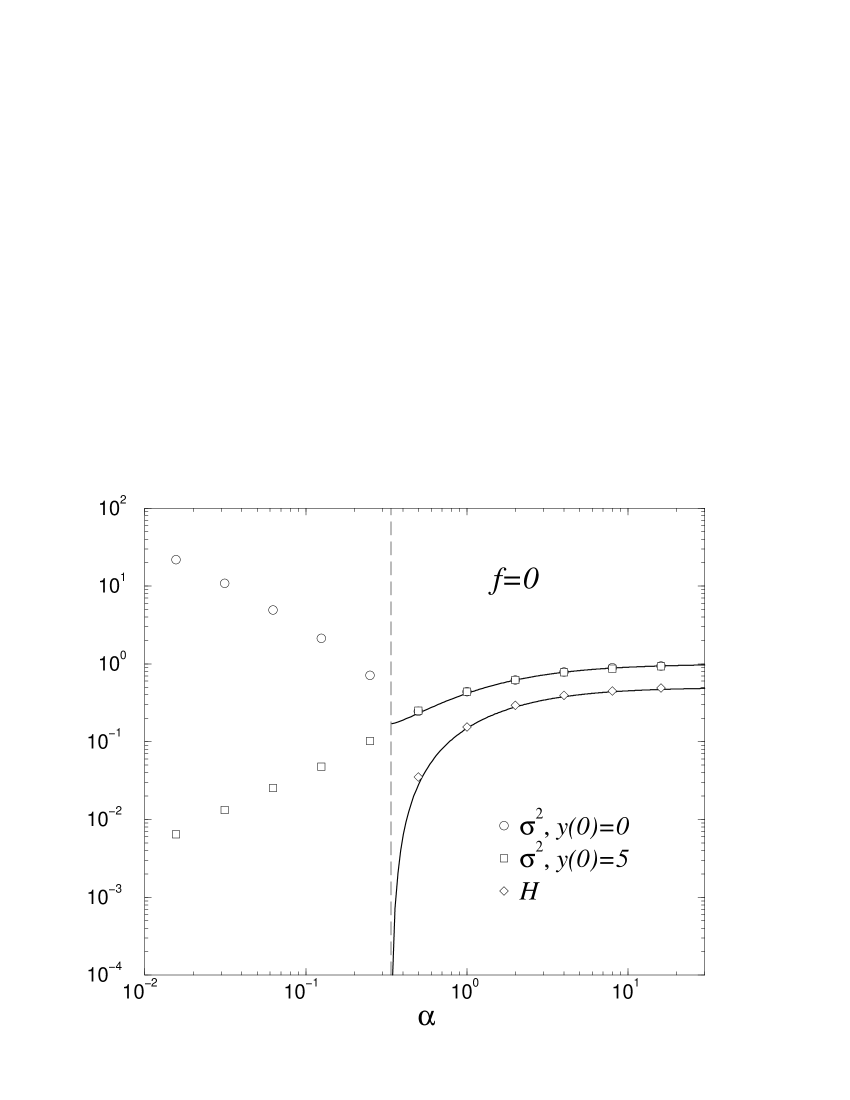
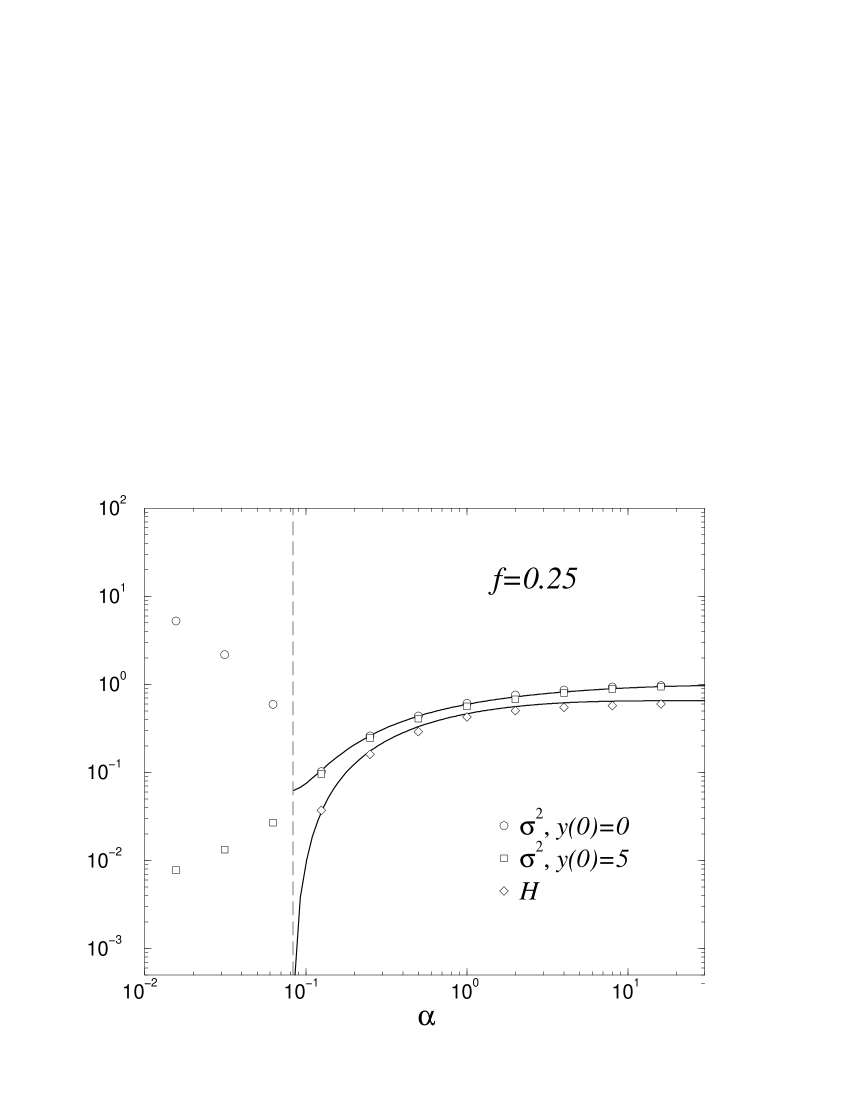
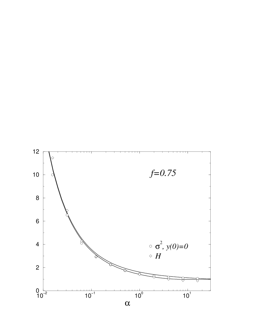
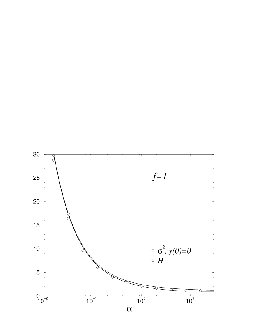
Figure 1: Behavior of $\sigma^{2}$ and $H$ vs $\alpha$ for $f=0,0.25,0.75,1$. Markers represent results from numerical simulations with homogeneous initial conditions, averaged over 200 disorder samples. The dashed vertical lines give the location of $\alpha_{c}$ (from theory). Continuous lines represent analytical approximations (valid only for $\alpha>\alpha_{c}$). Results for $H$ are compared with the static approximation of Sec. 3, while those for $\sigma^{2}$ are compared with the dynamical results of Sec. 4. The logarithmic scale on the $y$-axis in the upper panels has been used to stress the dependence of $\sigma^{2}$ on the initial conditions for $\alpha<\alpha_{c}$. In the lower panels, the upper curves correspond in both figures to the static results for $H$.

For $f<1/2$, a minority-game type of behavior is recovered, with an asymmetric phase ($H>0$) at high $\alpha$ separated by a symmetric one ($H=0$) at low $\alpha$. The transition point $\alpha_{c}$ decreases as $f$ increases, hence the symmetric phase shrinks as more and more trend-followers join the game, indicating that they provide an additional exploitable ‘signal’. Market fluctuations tend to the random limit $\sigma^{2}=1$ for large $\alpha$ and decrease with $\alpha$ until the critical point is reached. In the sub-critical phase, the stationary state depends strongly on the initial conditions of (3), and both high-volatility and low-volatility states can be reached starting from slightly different configurations. For $f>1/2$, instead, trend-followers dominate the game and the global efficiency decreases steadily with $\alpha$ and $f$. The market is asymmetric ($H>0$) for all $\alpha$ and the difference between $\sigma^{2}$ and $H$ diminishes as $f$ increases. For $f=1$, one has $\sigma^{2}=H$. The dependence of $\sigma^{2}$ on the initial conditions is arguably very weak (obviously provided initial conditions are not too biased). The case $f=1/2$ possesses some special features and will be treated separately [23].

In order to get some theoretical insight, one can follow the line of reasoning adopted for the pure minority game, for which it was shown by constructing the continuous-time limit of (3) that the average asymptotic value of $s_{i}$, denoted by $m_{i}$, can be obtained by minimizing the random function

$$\mathcal{H}(\boldsymbol{m})=\frac{N}{P}\sum_{\mu=1,P}[\Omega^{\mu}+\frac{1}{\sqrt{N}}\sum_{i=1,N}\xi_{i}^{\mu}m_{i}]^{2}$$ (6)

where $\boldsymbol{m}=\{m_{i}\}$. (Notice that the $m_{i}$’s are ‘soft’ spin: $-1\leq m_{i}\leq 1$.) We will not discuss here the limitations of this approximation and refer the reader to the original literature [13, 24, 25, 26, 27, 28, 29] for a critical discussion. In the limit $N\to\infty$, this problem could be tackled using spin-glass techniques, because

$$\lim_{N\to\infty}\min_{\boldsymbol{m}}~{}\frac{\mathcal{H}(\boldsymbol{m})}{N}=-\lim_{\beta\to\infty}\lim_{N\to\infty}\frac{1}{\beta N}~{}\overline{\log Z(\beta)}$$ (7)

(here, $Z(\beta)=\int e^{-\beta\mathcal{H}}d\boldsymbol{m}$ and the over-line denotes an average over disorder). The evaluation of $\overline{\log Z}$ requires the replica trick [30]. For $\alpha>\alpha_{c}$, $\mathcal{H}$ has a unique minimum, hence the stationary state can be fully described by the replica-symmetric solution of (7).

This argument can be easily reformulated for the pure majority game. The corresponding optimization problem turns out to be

$$\max_{\boldsymbol{m}}~{}\mathcal{H}(\boldsymbol{m})\quad{\rm~{}or,equivalently,}\quad\min_{\boldsymbol{m}}~{}-\mathcal{H}(\boldsymbol{m})$$ (8)

A few comments are in order. First, it is easy to see that $H=\mathcal{H}/N$, which implies that minority game players roughly tend to minimize the available information, while majority ones tend to maximize it. Second, at odds with $\mathcal{H}$, $-\mathcal{H}$ possesses many minima, hence the stationary state of the majority game will always depend on the initial conditions of the dynamics (even though the macroscopic observables $\sigma^{2}$ and $H$ might take on the same or very similar values in all minima). Basing on well-known properties of the Hopfield model [10], one expects the true minima of $-\mathcal{H}$ to be described by solutions of (8) that break replica symmetry. Moreover, as happens in attractor neural networks with extensively many patterns, a “retrieval” phase is to be expected for small enough $\alpha$ where, due to correlations between the initial conditions and one specific pattern, say $\mu=1$, the overlap $o^{\mu}(\boldsymbol{m})=N^{-1/2}\sum_{i=1,N}\xi_{i}^{\mu}m_{i}$ is $\Or(N^{-1/2})$, and vanishing as $N\to\infty$, for all $\mu$’s except $\mu=1$, for which it is finite. The fact that agents can ‘condense’ around a given pattern implies that every time that pattern is presented to them a buy (or sell) rush takes place. Solving (8) is hence a non-trivial task in itself, and requires a detailed study [12].

Generalizing to our case, one finds that the stationary $m_{i}$’s for the mixed majority-minority model can be obtained by solving the following problem:

$$\max_{\boldsymbol{m}_{2}}~{}\min_{\boldsymbol{m}_{1}}~{}\mathcal{H}(\boldsymbol{m}_{1},\boldsymbol{m}_{2})$$ (9)

where $\boldsymbol{m}_{1}$ (resp. $\boldsymbol{m}_{2}$) denote collective the $m_{i}$ variables of minority (resp. majority) game players. Hence the mixed game where both minority and majority players are present at the same time requires a minimization of $\mathcal{H}$ in certain directions (the minority ones) and a maximization in others (the majority ones). Again, this problem can be tackled by a replica theory. The idea [14] is to introduce two ‘inverse temperatures’ $\beta_{1}$ and $\beta_{2}$ for minority and majority players respectively, such that

$$\max_{\boldsymbol{m}_{2}}~{}\min_{\boldsymbol{m}_{1}}~{}\mathcal{H}(\boldsymbol{m}_{1},\boldsymbol{m}_{2})=\lim_{\beta_{1},\beta_{2}\to\infty}\frac{1}{\beta_{2}}~{}\overline{\log\mathcal{Z}(\beta_{1},\beta_{2})}$$ (10)

with the following generalized partition function:

$$\mathcal{Z}(\beta_{1},\beta_{2})=\int d\boldsymbol{m}_{2}~{}e^{\beta_{2}\left[-\frac{1}{\beta_{1}}\log\int d\boldsymbol{m}_{1}~{}e^{-\beta_{1}\mathcal{H}}\right]}=\int d\boldsymbol{m}_{2}\left[\int d\boldsymbol{m}_{1}~{}e^{-\beta_{1}\mathcal{H}}\right]^{-\gamma}$$ (11)

where $\gamma=\beta_{2}/\beta_{1}>0$. In physical jargon, this describes a system where: first, the $\boldsymbol{m}_{1}$ variables are thermalized at a positive temperature $1/\beta_{1}$ with Hamiltonian $\mathcal{H}$ at fixed $\boldsymbol{m}_{2}$; then, the $\boldsymbol{m}_{2}$ variables are thermalized at a negative temperature $-1/\beta_{2}$ with an effective Hamiltonian $\mathcal{H}_{{\rm eff}}$ defined by $-\beta_{1}\mathcal{H}_{{\rm eff}}(\boldsymbol{m}_{2})=\log\int d\boldsymbol{m}_{1}~{}e^{-\beta_{1}\mathcal{H}}$. The disorder average can be carried out with the help of a ‘nested’ replica trick. First, one replicates the minority variables by treating the exponent $-\gamma$ as a positive integer $R$ (in the end, the limit $R\to-\gamma<0$ must be taken). (11) thus becomes

$$\mathcal{Z}=\int d\boldsymbol{m}_{2}\left[\int d\boldsymbol{m}_{1}~{}e^{-\beta_{1}\mathcal{H}}\right]^{R}=\int d\boldsymbol{m}_{2}\left[\int e^{-\beta_{1}\sum_{r}\mathcal{H}(\{\boldsymbol{m}_{1}^{r}\},\boldsymbol{m}_{2})}\prod_{r=1,R}d\boldsymbol{m}_{1}^{r}\right]$$ (12)

Then a second replication is needed, this time on the $\boldsymbol{m}_{2}$ variables:

$$\mathcal{Z}^{n}=\int e^{-\beta_{1}\sum_{a,r}\mathcal{H}(\{\boldsymbol{m}_{1}^{ar}\},\{\boldsymbol{m}_{2}^{a}\})}\prod_{a=1,n}\prod_{r=1,R}d\boldsymbol{m}_{1}^{ar}d\boldsymbol{m}_{2}^{a}$$ (13)

At this point we have two replica indexes with different roles: the $a$ replicas have been introduced to deal with the disorder, and their number $n$ will eventually go to zero, as usual; the $r$ replicas have been introduced to deal with the negative temperature, and their number $R$ must be set to a negative value. Majority variables bear just one index, while minority ones have two. We can interpret this fact by saying that $\boldsymbol{m}_{2}^{a}$ indicates a particular configuration of the majority variables, i.e. a given manifold in the whole $\boldsymbol{m}$ space; and $\boldsymbol{m}_{1}^{ar}$ indicates the minority coordinates in that particular manifold.

In Sec. 3 we will solve (10) in the limit $N\to\infty$ using (13) as a starting point. Evidently, retrieval solutions for the majority part become increasingly important as $f$ gets bigger. We will however neglect this aspect (which in the mixed case leads to a serious lengthening). Results obtained in this way give a very good agreement with numerical simulations, suggesting that retrieval doesn’t substantially affect the average macroscopic properties of the game. Of course, it is expected to play a very important role for phenomena that are local in time (like “bubbles”). Besides this static approximation, we will also tackle the dynamics (3) straightforwardly, resorting to the generating-functional method to carry out the disorder-average. Again, we will neglect the possibility of retrieval. Following [17], we will focus on the ‘batch’ version of the model. Dynamical results obtained in this way turn out to coincide nicely with their static counterpart and suggest that the transition occurring at $\alpha_{c}$ for $f<1/2$ is related essentially to the onset of anomalous response, as in the pure minority game. We will calculate the critical line $\alpha_{c}(f)$, showing that $\alpha_{c}\downarrow 0$ as $f\uparrow 1/2$. For $f>1/2$, the response is always finite and the macroscopic properties are dominated by the contribution of trend followers.

3 Statics

To begin, let us re-write the Hamiltonian (6) as

$$\mathcal{H}(\boldsymbol{m}_{1},\boldsymbol{m}_{2})=\frac{1}{P}\sum_{\mu=1,P}\left[\sum_{i=1,N}\omega_{i}^{\mu}+\sum_{j\in N_{1}}\xi_{j}^{\mu}m_{1j}+\sum_{k\in N_{2}}\xi_{k}^{\mu}m_{2k}\right]^{2}$$ (14)

where $N_{1}$ (resp. $N_{2}$) denotes both the set and the cardinality of the set of minority (resp. majority) game players. The replicated Hamiltonian entering (13) is

$$\mathcal{H}(\{\boldsymbol{m}_{1}^{ar}\},\{\boldsymbol{m}_{2}^{a}\})=\frac{1}{P}\sum_{\mu=1,P}\left[\sum_{i=1,N}\omega_{i}^{\mu}+\sum_{j\in N_{1}}\xi_{j}^{\mu}m_{1j}^{ar}+\sum_{k\in N_{2}}\xi_{k}^{\mu}m_{2k}^{a}\right]^{2}$$ (15)

We can as usual linearize the exponential in (13) via a Hubbard-Stratonovich transformation introducing some auxiliary Gaussian variables $z_{ar}^{\mu}$. Subsequently, the average over the disorder can be easily performed using the distribution $P(a_{ig}^{\mu})=1/2(\delta_{a_{ig}^{\mu},1}+\delta_{a_{ig}^{\mu},-1})$ ($g=1,2$) and the definitions of $\omega_{i}^{\mu}$ and $\xi_{i}^{\mu}$. One obtains

$$\overline{\mathcal{Z}^{n}}=\int[\prod_{a,r}d\boldsymbol{m}_{1}^{ar}d\boldsymbol{m}_{2}^{a}][\prod_{\mu,a,r}\frac{dz_{ar}^{\mu}}{\sqrt{2\pi}}]~{}e^{-\sum_{\mu}\sum_{ar}\frac{(z_{ar}^{\mu})^{2}}{2}}\times$$ (16)

$$\times e^{-\frac{\beta_{1}}{2\alpha}\sum_{\mu}\sum_{abrs}z_{ar}^{\mu}z_{bs}^{\mu}(1+(1-f)\frac{1}{N_{1}}\sum_{j\in N_{1}}m_{1j}^{ar}m_{1j}^{bs}+f\frac{1}{N_{2}}\sum_{k\in N_{2}}m_{2k}^{a}m_{2k}^{b})}$$

It is now convenient to define the overlaps

$$Q_{ar,bs}=\frac{1}{N_{1}}\sum_{j\in N_{1}}m_{1j}^{ar}m_{1j}^{bs}\quad{\rm and}\quad P_{ab}=\frac{1}{N_{2}}\sum_{k\in N_{2}}m_{2k}^{a}m_{2k}^{b}$$ (17)

inserting them in (16) via $\delta$-distributions with Lagrange multipliers $\widehat{Q}_{ab,rs}$ and $\widehat{P}_{ab}$. Notice that the overlap matrices $\mathsf{Q}$ and $\mathsf{P}$ are $nR$-dimensional and $n$-dimensional, respectively. In this way the site dependence can be easily dealt with, so that after a little algebra one gets (all numerical factors are ‘hidden’ in the $D(\cdot,\cdot)$ shorthand):

$$\overline{\mathcal{Z}^{n}}=\int e^{NS(\mathsf{Q},\mathsf{\widehat{Q}},\mathsf{P},\mathsf{\widehat{P}})}~{}D(\mathsf{Q},\mathsf{\widehat{Q}})D(\mathsf{P},\mathsf{\widehat{P}})$$ (18)

where the effective action $S$ is given by ($a,b=1,\ldots,nR~{}$; $~{}r,s=1,\ldots,R$)

$$S(\mathsf{Q},\mathsf{\widehat{Q}},\mathsf{P},\mathsf{\widehat{P}})=-\frac{\alpha}{2}\log\det\mathsf{T}-{\rm i}~{}[(1-f)\Tr(\mathsf{\widehat{Q}}\mathsf{Q})+f\Tr(\mathsf{\widehat{P}}\mathsf{P})]+$$

$$+(1-f)\log\int_{-1}^{+1}[\prod_{a,r}dm_{1}^{a,r}]~{}e^{{\rm i}\sum_{abrs}m_{1}^{ar}\widehat{Q}_{ar,bs}m_{1}^{bs}}+f\log\int_{-1}^{+1}[\prod_{a}dm_{2}^{a}]~{}e^{{\rm i}\sum_{ab}m_{2}^{a}\widehat{P}_{ab}m_{2}^{b}}$$

with

$$\mathsf{T}=\mathsf{I}_{nR}+\frac{\beta_{1}}{\alpha}[\mathsf{E}_{nR}+(1-f)\mathsf{Q}+f\mathsf{P}\otimes\mathsf{E}_{R}]$$ (19)

$\mathsf{I}_{K}$ stands for the $K\times K$ identity matrix while $\mathsf{E}_{K}$ denotes the $K\times K$ matrix with all elements equal to $1$. $\otimes$ is the Kronecker product. In (3) one can easily recognize some parts coming from the minority agents (those proportional to $(1-f)$) and others coming from the majority agents. These contributions are not factorized (in that event, the mixed problem would be trivial) but are interconnected via the determinant of $\mathsf{T}$.

To proceed further, one has to formulate Ansätze for the overlap matrices and then perform the integral (18) in the limit $N\to\infty$ by the steepest descent method. Let us first arrange $\mathsf{Q}$ in a convenient matrix form. We choose to order the indexes in such a way that each row is characterized by a couple $(a,r)$; along the row, the index $a$ is first kept fixed while $r$ varies from $1$ to $R$. $\mathsf{Q}$ is thus naturally subdivided in blocks of size $R\times R$, the blocks along the diagonal corresponding to a given value of $a=b$. We remind that keeping $a$ fixed corresponds to selecting, in the global configuration space, a well defined manifold with $\boldsymbol{m}_{2}=\boldsymbol{m}_{2}^{a}$ inside which $\mathcal{H}$ is minimized with respect to the $\boldsymbol{m}_{1}$ variables. $Q_{ar,as}$ can be thus interpreted as the overlap between two configurations of the same constrained minority problem. It is natural to assume for these diagonal sub-blocks the same matrix structure of a pure minority game, that is a symmetric form with a diagonal element $Q$ and an off-diagonal one $q_{1}$. On the other hand, elements of the type $Q_{ar,bs}$ with $a\neq b$ correspond to overlaps between two minority configurations in different majority manifolds, and the simplest choice one can make is to take $Q_{ar,bs}=q_{0}$ for all of them. In this way $\mathsf{Q}$ assumes what is called a 1-step RSB (replica symmetry broken) form [30]:

$$Q_{ar,bs}=(Q-q_{1})\delta_{ab}\delta_{rs}+(q_{1}-q_{0})\epsilon_{arbs}+q_{0}$$ (20)

where the tensor $\epsilon_{arbs}$ is equal to $1$ in the diagonal $R\times R$ blocks with $a=b$, and $0$ elsewhere. Notice that, contrary to standard replica calculations, here the block size $R$ is not a variational parameter, but its value is fixed by the nature of the problem. For consistency, we adopt the same Ansatz for the conjugated matrix $\widehat{\mathsf{Q}}$. The choice for the $n\times n$ matrices $\mathsf{P}$ and $\widehat{\mathsf{P}}$ is on the other hand more straightforward: we will consider the simple replica-symmetric Ansatz

$$P_{ab}=(P-p_{0})\delta_{ab}+p_{0}$$ (21)

and take an analogous form for $\widehat{\mathsf{P}}$.

Putting (20) and (21) into (3), and using the conventional re-scalings $\mathsf{\widehat{Q}}=(-i\beta_{1}^{2}\alpha/2)\mathsf{\Omega}$ and $\mathsf{\widehat{P}}=(-i\beta_{1}^{2}\alpha/2)\mathsf{G}$, the ‘free energy’ density $F=-S/(\beta_{1}n)$ turns out to be given, in the limit $n\to 0$, by

$$F=\frac{\alpha R}{2\beta_{1}}\log\left[1+(1-f)\frac{\beta_{1}}{\alpha}(Q-q_{1})\right]+\frac{\beta_{1}R\alpha(1-f)}{2}\left[\Omega Q+(R-1)\omega_{1}q_{1}-R\omega_{0}q_{0}\right]+$$

$$+\frac{\alpha}{2\beta_{1}}\log\left[1+R\beta_{1}\frac{(1-f)(q_{1}-q_{0})+f\ (P-p_{0})}{\alpha+(1-f)\beta_{1}(Q-q_{1})}\right]+\frac{\beta_{1}\alpha}{2}f(GP-g_{0}p_{0})+$$

$$+\frac{\alpha R}{2}\frac{1+(1-f)q_{0}+fp_{0}}{\left[\alpha+(1-f)\beta_{1}(Q-q_{1})\right]\left[R\beta_{1}(1-f)(q_{1}-q_{0})+f(P-p_{0})\right]}+$$ (22)

$$-\frac{1-f}{\beta_{1}}\int dz\mathcal{P}(z)\log\int dy\mathcal{P}(y)\left[\int_{-1}^{1}dm_{1}~{}e^{-\beta_{1}V_{zy}(m_{1})}\right]^{R}+$$

$$-\frac{f}{\beta_{1}}\int dz\mathcal{P}(z)\log\int_{-1}^{1}dm_{2}~{}e^{-\beta_{1}V_{z}(m_{2})}$$

where $\mathcal{P}(x)=e^{-x^{2}/2}/\sqrt{2\pi}$ and

$$V_{zy}(m_{1})=-z\sqrt{\alpha\omega_{0}}ym_{1}\sqrt{\alpha(\omega_{1}-\omega_{0})}-\frac{\alpha\beta_{1}}{2}(\Omega-\omega_{1})m_{1}^{2}$$ (23)

$$V_{z}(m_{2})=-\sqrt{\alpha g_{0}}zm_{2}-\frac{\alpha\beta_{1}}{2}(G-g_{0})m_{2}^{2}$$ (24)

The replica recipe now prescribes an extremization of (3) with respect to its ten variational parameters (namely $Q$, $q_{0}$, $q_{1}$, $P$, $p_{0}$ and their conjugate variables), because when $N\to\infty$ it is easy to see that

$$\lim_{N\to\infty}\max_{\boldsymbol{m}_{2}}~{}\min_{\boldsymbol{m}_{1}}~{}\frac{\mathcal{H}}{N}=\lim_{\beta_{1},\beta_{2}\to\infty}\frac{F({\rm saddle~{}point})}{R}$$ (25)

This leaves us with a set of ten equations in ten variables. Defining

$$\chi_{1}=\frac{\beta_{1}}{\alpha}(Q-q_{1})-\frac{\beta_{2}}{\alpha}(q_{1}-q_{0})$$ (26)

$$\chi_{2}=\frac{\beta_{2}}{\alpha}(P-p_{0})$$ (27)

$$\chi=(1-f)\chi_{1}-f\chi_{2}$$ (28)

and using the shorthands

$$\left\langle\!\left\langle{\cdots}\right\rangle\!\right\rangle=\int dz\mathcal{P}(z)\left[\frac{\int dy\mathcal{P}(y)\left[\mathcal{Q}^{R-1}\int_{-1}^{1}dm_{1}~{}\cdots~{}e^{-\beta_{1}V_{yz}(m_{1})}\right]}{\int dy\mathcal{P}(y)\left[\mathcal{Q}^{R}\right]}\right]$$ (29)

$\mathcal{Q}=\int_{-1}^{1}dm_{1}~{}e^{-\beta_{1}V_{yz}(m_{1})}$ being a normalization integral, and

$$\left\langle{\cdots}\right\rangle_{2}=\frac{\int_{-1}^{1}dm_{2}~{}\cdots~{}e^{-\beta_{1}V_{z}(m_{2})}}{\int_{-1}^{1}dm_{2}~{}e^{-\beta_{1}V_{z}(m_{2})}}$$ (30)

we find the following system:

$$Q=\left\langle\!\left\langle{m_{1}^{2}}\right\rangle\!\right\rangle$$ (31)

$$\beta_{1}Rq_{1}+\beta_{1}(Q-q_{1})=\frac{\left\langle\!\left\langle{ym_{1}}\right\rangle\!\right\rangle}{\sqrt{\alpha(\omega_{1}-\omega_{0})}}$$ (32)

$$\alpha\chi_{1}=\frac{\left\langle\!\left\langle{zm_{1}}\right\rangle\!\right\rangle}{\sqrt{\alpha\omega_{0}}}$$ (33)

$$\beta_{1}(\Omega-\omega_{1})=-\frac{1}{\alpha+\beta_{1}(1-f)(Q-q_{1})}$$ (34)

$$\omega_{1}-\omega_{0}=\frac{(1-f)(q_{1}-q_{0})+f(P-p_{0})}{\alpha(1+\chi)[\alpha+\beta_{1}(1-f)(Q-q_{1})]}$$ (35)

$$\omega_{0}=\frac{1+(1-f)q_{0}+fp_{0}}{\alpha^{2}(1+\chi)^{2}}$$ (36)

$$P=\left\langle{m_{2}^{2}}\right\rangle_{2}$$ (37)

$$g_{0}=R^{2}\omega_{0}$$ (38)

$$\alpha\chi_{2}=-R\frac{\left\langle{zm_{2}}\right\rangle_{2}}{\sqrt{\alpha g_{0}}}$$ (39)

$$\beta_{1}(G-g_{0})=-\frac{R}{\alpha(1+\chi)}$$ (40)

Some observations about these equations are in order. First, if we set $f=0$ we recover exactly the saddle point equations for a pure minority game problem at inverse temperature $\beta_{1}$. For what concerns the $\chi$’s, it will soon become clear that $\chi_{1}$ is the susceptibility of minority agents and, when $f=0$, it reproduces the susceptibility of a pure minority game, while $\chi_{2}$ is the susceptibility of majority agents. On the other hand, $\chi$ is evidently not the global susceptibility. This is a consequence of the fact that to treat minority and majority players within the same formalism we had to introduce the effective negative inverse temperature $-\beta_{2}$.

Solving the above system at finite temperature(s) is a quite difficult task. Fortunately, in this case we are only interested in the limit of zero temperature(s), in which the solution of (31–40) turn out not to depend explicitly on $R$, provided $G$ and $g_{0}$ are rescaled by $R^{2}$. Specifically, we look for solutions with $q_{0}\to q_{1}\to Q$ and $p_{0}\to P=1$ such that $\chi_{1}$, $\chi_{2}$ and $\chi$ remain finite. These assumptions are justified for minority variables by the existence of just one global minimum of $\mathcal{H}$ (which also means that the minimum is unique in each manifold with given $\boldsymbol{m}_{2}$). On the other hand, they are more questionable for majority variables, since the maxima of $\mathcal{H}$ are numerous and disconnected (they occur evidently in the corner of the configuration space $[-1,1]^{N}$). However, they are the simplest possible in absence of retrieval states. We will adopt them for this reason, but it should be kept in mind that they may not be the most appropriate ones in general.

After some algebra, the set of saddle point equations can be greatly simplified, because, as in [21], when $\beta_{1},\beta_{2}\to\infty$ the averages (29) and (30) can be explicitly performed by steepest descent. The result for the relevant quantities is

$$P=1$$ (41)

$$Q=1-\sqrt{\frac{2}{\pi}}\frac{e^{-\frac{\lambda^{2}}{2}}}{\lambda}-\left(1-\frac{1}{\lambda^{2}}\right){\rm erf}\frac{\lambda}{\sqrt{2}}$$ (42)

$$\frac{\alpha\chi}{1+\chi}=(1-f){\rm erf}\frac{\lambda}{\sqrt{2}}-f\sqrt{\frac{2}{\pi}}\lambda$$ (43)

with $\lambda=\sqrt{\alpha/[1+(1-f)Q+f]}$. The identity $P=1$ implies that majority agents use only one of their strategies, i.e. that the stationary state of a pure majority game is in pure strategies. We define

$$c=(1-f)Q+f$$ (44)

Evidently, $H$ can be expressed in terms of all saddle-point values since $\mathcal{H}/N=H$. Using (25) and taking the limit $R\to-1$ (this is equivalent to taking the limit $\beta_{1}\to\beta_{2}$ followed by $\beta_{2}\to\infty$) one easily finds

$$H=\frac{1+c}{2(1+\chi)^{2}}$$ (45)

The existence of a transition at some critical value of $\alpha$ is determined by the divergence of $\chi$ (which means that $H$ becomes $0$). From (43) we find for $\alpha_{c}$ the following expression:

$$\alpha_{c}(f)=(1-f){\rm erf}(x)-\frac{2fx}{\sqrt{\pi}}$$ (46)

where $x$ is the solution of

$$2-(1-f){\rm erf}(x)-\frac{1-f}{x\sqrt{\pi}}e^{-x^{2}}+\frac{f}{x\sqrt{\pi}}=0$$ (47)

Solving the above equations numerically for different $f$ one obtains a very good agreement with the behavior of $H$ (see Fig. 1). The critical line $\alpha_{c}$ calculated from (46,47) is instead displayed in Fig. 2.

Figure 2: Critical line separating the asymmetric, inefficient phase with $H>0$ from the symmetric one with $H=0$ in the $(f,\alpha)$ plane. As $\alpha\downarrow\alpha_{c}(f)$, $\chi\to\infty$.

It should be mentioned that an approximate expression for $\sigma^{2}$ can also be obtained, $\sigma^{2}\simeq H+(1-c)/2$, but it is not as accurate as the one for $H$. A better estimate of $\sigma^{2}$ is obtained by solving the dynamics. As a last remark, let us notice that for a pure majority game one gets, from (36–39) and from the fact that $\left\langle{zm_{2}}\right\rangle_{2}=\sqrt{2/\pi}$,

$$\chi_{2}=\frac{1}{1+\sqrt{\alpha\pi}}\quad{\rm and}\quad H=(1-\chi_{2})^{-2}$$ (48)

The expression for $\chi_{2}$ is identical to that of the Hopfield model at zero temperature.

4 Dynamics

Let us turn our attention to the dynamics. For simplicity, we concentrate on the ‘batch’ case [17], which is obtained by averaging (3) over the $\mu$’s and re-scaling time. This amounts to considering the case in which performance updates are made after many ($\Or(P)$) iterations rather than at end of every round. This approximation has already proved to be an extremely good one for minority games. One arrives at

$$y_{i}(t+1)-y_{i}(t)=\epsilon_{i}h_{i}+\epsilon_{i}\sum_{j=1,N}J_{ij}s_{j}(t)$$ (49)

where $h_{i}=(2/\sqrt{N})\sum_{\mu=1,P}\xi_{i}^{\mu}\Omega^{\mu}$ and $J_{ij}=(2/N)\sum_{\mu=1,P}\xi_{i}^{\mu}\xi_{j}^{\mu}$. The dynamical partition function of (49) reads

$$Z[\boldsymbol{\psi}]=\left\langle{e^{{\rm i}\sum_{it}y_{i}(t)\psi_{i}(t)}}\right\rangle_{{\rm paths}}$$

$$=\int e^{{\rm i}\sum_{it}\widehat{y}_{i}(t)\left[y_{i}(t+1)-y_{i}(t)-\epsilon_{i}h_{i}-\epsilon_{i}\sum_{j}J_{ij}s_{j}(t)-\theta_{i}(t)\right]+y_{i}(t)\psi_{i}(t)}p(\boldsymbol{y}(0))D(\boldsymbol{y},\boldsymbol{\widehat{y}})$$ (50)

where $D(\boldsymbol{y},\boldsymbol{\widehat{y}})=\prod_{it}[dy_{i}(t)d\widehat{y}_{i}(t)/(2\pi)]$ and $\theta_{i}$ is a time-dependent external field. In principle, disorder-averaged correlation and response functions can be calculated exactly at all times by taking appropriate derivatives of the disorder-averaged $Z$, i.e.

$$\overline{Z[\boldsymbol{\psi}]}=\int e^{{\rm i}\sum_{it}\widehat{y}_{i}(t)\left[y_{i}(t+1)-y_{i}(t)-\theta_{i}(t)\right]+y_{i}(t)\psi_{i}(t)+NF(\boldsymbol{\widehat{y}})}p(\boldsymbol{y}(0))D(\boldsymbol{y},\boldsymbol{\widehat{y}})$$ (51)

$$F(\boldsymbol{\widehat{y}})=\frac{1}{N}\log\overline{\left[e^{-{\rm i}\sum_{it}\widehat{y}_{i}(t)\epsilon_{i}\left[h_{i}+\sum_{j}J_{ij}s_{j}(t)\right]}\right]}$$ (52)

with respect to the fields $\psi_{i}$ and $\theta_{i}$. We shall however be interested in the stationary state only. As usual, evaluation of $\overline{Z}$ leads to an effective (non-Markovian) process that provides an equivalent description of the original (Markovian) multi-agent process (49). Such a calculation is in this case rather similar to that done for the pure batch minority game in [17], and is sketched in the Appendix. The main difference is that here we obtain two effective processes, describing trend-followers and fundamentalists respectively. These are given by

$$y(t+1)-y(t)=\alpha\epsilon\sum_{t^{\prime}}[(\mathsf{I}+\mathsf{G})^{-1}]_{tt^{\prime}}s(t^{\prime})+\theta(t)+\sqrt{\alpha}z(t)$$ (53)

where $\epsilon=1$ (resp. $-1$) for the majority (resp. minority) part, and $z(t)$ is a zero-average Gaussian random variable with temporal correlations

$$\left\langle{z(t)z(t^{\prime})}\right\rangle=[(\mathsf{I}+\mathsf{G})^{-1}(\mathsf{E}+\mathsf{C})(\mathsf{I}+\mathsf{G}^{T})^{-1}]_{tt^{\prime}}$$ (54)

$\mathsf{I}$ stands for the identity matrix while $\mathsf{E}$ denotes the matrix with all elements equal to one. $\mathsf{C}$ has elements $C_{tt^{\prime}}=\left\langle{s(t)s(t^{\prime})}\right\rangle$. $\mathsf{G}$, instead (see Appendix for details), is the sum of two contributions:

$$\mathsf{G}=(1-f)\mathsf{G}_{1}-f\mathsf{G}_{2}$$ (55)

$\mathsf{G}_{1}$ (resp. $\mathsf{G}_{2}$) has elements $\left\langle{\partial s(t)/\partial\theta(t^{\prime})}\right\rangle_{-1}$ (resp. $\left\langle{\partial s(t)/\partial\theta(t^{\prime})}\right\rangle_{+1}$) where the subscript means average over the process (53) with $\epsilon=-1$ (resp. $+1$). When $N\to\infty$, $C_{tt^{\prime}}$ can be identified with the disorder- and agent-averaged autocorrelation function of (49), while the two components of $G_{tt^{\prime}}$ become identical to the disorder- and agent-averaged response functions of minority and majority agents, respectively.

Ergodic stationary states can be studied under the following assumptions:

• Time-translation invariance (TTI): $\cases{\lim_{t\to\infty}C_{t+\tau,t}=C(\tau)\\ \lim_{t\to\infty}G_{t+\tau,t}=G(\tau)}$;

• Finite integrated ‘response’ (FIR): $\lim_{t\rightarrow\infty}\sum_{t^{\prime}\leq t}G_{tt^{\prime}}=\chi<\infty$;

• Weak long-term memory (WLTM): $\lim_{t\to\infty}G(t,t^{\prime})=0\quad\forall t^{\prime}$ finite.

The breakdown of any of these signals the breakdown of ergodicity. To be more clear, we remark that the ‘integrated response’ $\chi$ defined in FIR has two components, i.e., with obvious notation,

$$\chi=(1-f)\chi_{1}-f\chi_{2}$$ (56)

and can be negative. $\chi_{1}$ and $\chi_{2}$ are the actual susceptibilities of minority and majority agents, respectively. With FIR, we will require that both $\chi_{1}$ and $\chi_{2}$ are finite.

As in the minority game, for individual agents there are two possibilities: either $y_{i}(t)/t\to{\rm constant}\neq 0$ as $t\to\infty$, in which case they use only one of their strategies asymptotically (we call these agents “frozen”); or $y_{i}(t)/t\to 0$ as $t\to\infty$, in which case they keep flipping between their strategies even in the long run (we call these agents “fickle”). Macroscopic quantities can be obtained by separating the contributions of frozen and fickle agents.

Defining $\widetilde{y}=\lim_{t\to\infty}y(t)/t$, $s=\lim_{\tau\to\infty}(1/\tau)\sum_{t\leq\tau}{\rm sign}[y(t)/t]$ and $z=\lim_{\tau\to\infty}(1/\tau)\sum_{t\leq\tau}z(t)$, one has that

$$\widetilde{y}=\frac{\alpha\epsilon s}{1+\chi}+\sqrt{\alpha}z+\theta=\sqrt{\alpha}\epsilon\gamma s+\sqrt{\alpha}z+\theta$$ (57)

Let us assume that $\gamma>0$ (this assumption is verified a posteriori). For minority game players ($\epsilon=-1$), we have a frozen agent (with $s={\rm sign}(\widetilde{y})$) if $|z|>\gamma$ and a fickle or non-frozen agent (with $s=z/\gamma$) if $|z|<\gamma$ [17]. In the majority part, all agents turn out to be frozen. In particular, for $z>\gamma$ agents freeze at $s=1$, for $z<-\gamma$ they freeze at $s=-1$, while for $|z|<\gamma$ they can freeze at either values of $s$. It follows that the average autocorrelation $c=\lim_{\tau\to\infty}\frac{1}{\tau}\sum_{t\leq\tau}C(t)$ is given by, separating the contributions of minority agents from majority agents ($\left\langle{~{}}\right\rangle=$ average over Gaussian r.v. $z$ with variance $\left\langle{z^{2}}\right\rangle=\lim_{\tau,\tau^{\prime}\to\infty}(\tau\tau^{\prime})^{-1}\sum_{t\leq\tau,t^{\prime}\leq\tau^{\prime}}[(\mathsf{I}+\mathsf{G})^{-1}(\mathsf{E}+\mathsf{C})(\mathsf{I}+\mathsf{G}^{T})^{-1}]_{tt^{\prime}}=(1+\chi)^{-2}(1+c)$):

$$c =(1-f)\left[\left\langle{\theta(|z|-\gamma)}\right\rangle+\left\langle{\theta(\gamma-|z|)\frac{z}{\gamma}}\right\rangle\right]+f$$ (58)

$$=(1-f)\left[1-{\rm erf}\frac{\lambda}{\sqrt{2}}+\frac{1}{\lambda^{2}}\left({\rm erf}\frac{\lambda}{\sqrt{2}}-\lambda\sqrt{\frac{2}{\pi}}e^{-\lambda^{2}/2}\right)\right]+f$$

where $\lambda=\sqrt{\frac{\alpha}{1+c}}$. This agrees with the replica result (44). For the fraction $\phi$ of frozen agents one obtains

$$\phi=(1-f)\left\langle{\theta(|z|-\gamma)}\right\rangle+f=1-(1-f){\rm erf}\frac{\lambda}{\sqrt{2}}$$ (59)

In Fig. 3 analytical results for $c$ and $\phi$ are compared with simulations.

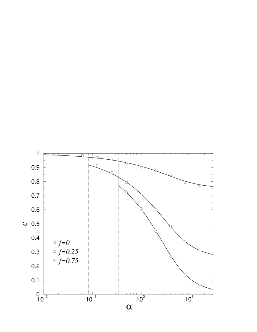
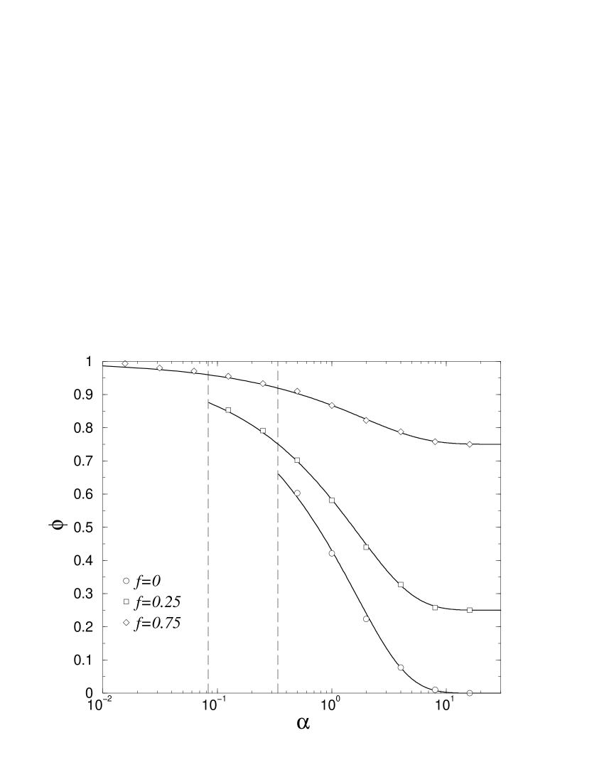
Figure 3: Persistent autocorrelation $c$ (left) and fraction of frozen agents $\phi$ (right) for various $f$. Lines correspond to the analytic solutions from (58) and (59), markers are the results from numerical simulations. Vertical lines give, for $f<1/2$, the position of the critical points $\alpha_{c}$ below which the stationary state (hence $c$ and $\phi$) depends on initial conditions.

The ‘susceptibility’ (56) can instead be calculated from the formula

$$\chi=(1-f)\frac{\left\langle{sz}\right\rangle_{\rm min}}{\sqrt{\alpha}\left\langle{z^{2}}\right\rangle}-f\frac{\left\langle{sz}\right\rangle_{\rm maj}}{\sqrt{\alpha}\left\langle{z^{2}}\right\rangle}$$ (60)

which follows directly from the fact that response functions for minority (resp. majority) agents can be obtained as $\alpha^{-1/2}\left\langle{\partial{\rm sign}[y(t)]/\partial z(t^{\prime})}\right\rangle_{-1}$ (resp. $\alpha^{-1/2}\left\langle{\partial{\rm sign}[y(t)]/\partial z(t^{\prime})}\right\rangle_{+1}$), after an integration by parts and a time average [17]. The minority part is as usual given by

$$\left\langle{sz}\right\rangle_{\rm min}=\left\langle{\theta(|z|-\gamma)|z|}\right\rangle+\left\langle{\theta(\gamma-|z|)\frac{z^{2}}{\gamma}}\right\rangle=\frac{1+c}{\sqrt{\alpha}(1+\chi)}~{}{\rm erf}\frac{\lambda}{\sqrt{2}}$$ (61)

To calculate the majority part, one must fix the value of the product $sz$ for $-\gamma\leq z\leq\gamma$, where $s$ can be either $+1$ or $-1$ (for $|z|>\gamma$ one has $sz=|z|$ in any case). In principle, there are several possibilities. If one makes the ‘natural’ choice $s={\rm sign}(z)$, then

$$\left\langle{sz}\right\rangle_{\rm maj}=\left\langle{|z|}\right\rangle=\sqrt{\frac{2}{\pi}}\sqrt{\frac{1+c}{(1+\chi)^{2}}}$$ (62)

This leads to

$$\frac{\alpha\chi}{1+\chi}=(1-f){\rm erf}\frac{\lambda}{\sqrt{2}}-f\lambda\sqrt{\frac{2}{\pi}}$$ (63)

$\chi$ diverges (hence FIR is violated and ergodicity is broken) when the fraction $\overline{\phi}=1-\phi$ of fickle agents satisfies $\overline{\phi}=\alpha+f\lambda\sqrt{2/\pi}$ or, equivalently, at the critical values of $\alpha$ given by the equation

$$\alpha_{c}(f)=(1-f){\rm erf}(x)-\frac{2fx}{\sqrt{\pi}}$$ (64)

where $x$ is the solution of

$$2-(1-f){\rm erf}(x)-\frac{1-f}{x\sqrt{\pi}}e^{-x^{2}}+\frac{f}{x\sqrt{\pi}}=0$$ (65)

(63–65) are in full agreement with the replica results of Sec. 3.

Another possibility is to calculate $\left\langle{sz}\right\rangle_{\rm maj}$ without making any special assumption on $s$ for $-\gamma\leq z\leq\gamma$. This brings us to a situation where (62–64) are substituted respectively by

$$\left\langle{sz}\right\rangle_{\rm maj} =\left\langle{\theta(z+\gamma)z}\right\rangle-\left\langle{\theta(\gamma-z)z}\right\rangle=e^{-\lambda^{2}/2}\sqrt{\frac{2}{\pi}}\sqrt{\frac{1+c}{(1+\chi)^{2}}}$$ (66)

$$\frac{\alpha\chi}{1+\chi} =(1-f){\rm erf}\frac{\lambda}{\sqrt{2}}-f\lambda\sqrt{\frac{2}{\pi}}e^{-\lambda^{2}/2}$$ (67)

$$\alpha_{c}(f) =(1-f){\rm erf}(x)-\frac{2fx}{\sqrt{\pi}}e^{-x^{2}}$$ (68)

where $x$ now solves

$$2-(1-f){\rm erf}(x)-\frac{1-2f}{x\sqrt{\pi}}e^{-x^{2}}=0$$ (69)

The value of $\overline{\phi}$ at which $\chi$ diverges is now $\overline{\phi}=\alpha+f\lambda e^{-\lambda^{2}/2}\sqrt{2/\pi}$. Notice that the extra exponential factor one obtains in this way does not change numerical results for $\alpha_{c}$ significantly (the solution of (65) is in fact $\lesssim 0.3$, so $e^{-x^{2}}$ is always close to $1$). Notice also that for a purely majority game (recalling that $\chi_{2}=-\chi$) one gets for the susceptibility

$$\chi_{2}=\frac{e^{-\alpha/4}/\sqrt{\alpha\pi}}{1+e^{-\alpha/4}/\sqrt{\alpha\pi}}$$ (70)

instead of the Hopfield-like formula (48). In both cases, $\chi_{2}\to\infty$ when $\alpha\downarrow 0$.

For the stationary volatility, which reads [17]

$$\sigma^{2}=\frac{1}{2}\lim_{t\to\infty}[(\mathsf{I}+\mathsf{G})^{-1}(\mathsf{E}+\mathsf{C})(\mathsf{I}+\mathsf{G}^{T})^{-1}]_{tt}$$ (71)

one can use the approximate method of [17] to derive an expression in terms of the persistent parameters $\chi$ and $\phi$, which holds for $\alpha>\alpha_{c}$:

$$\sigma^{2}=\frac{1+\phi}{2(1+\chi)^{2}}+\frac{1}{2}(1-\phi)$$ (72)

Solving for $\chi$, $\phi$ and $c$ for different $f$ and substituting one obtains the volatility branches displayed in Fig. 1, which are again in excellent agreement with simulations.

5 Summary and outlook

To summarize, we have studied the mixed majority-minority game with random external information. Neglecting ‘retrieval’ (i.e. the possibility that trend-followers flock in presence of a particular information pattern), we have first calculated the stationary state of the dynamics from a static approximation via a negative-replica theory. Then we have solved the dynamics using generating functional methods. The two approaches match nicely and agree with numerical results for the macroscopic observables $\sigma^{2}$ and $H$ in a satisfactory way. This suggests that retrieval does not affect such quantities significantly. Our results also indicate that when fundamentalists outnumber trend-followers, the macroscopic behavior of the system (‘phase transition’ with ergodicity breaking from an inefficient phase at high $\alpha$ to an efficient one at low $\alpha$) can be explained by the onset of anomalous response, that is by a divergence of the integrated response, as in the pure minority game. We have calculated the line of critical points in the $(f,\alpha)$ plane showing that the inefficient phase gets larger as $f$ increases. When trend-followers dominate, instead, the system is always inefficient and low volatility states disappear. As a byproduct, we have provided an approximate static and dynamical solution of the majority game. A greater effort is nevertheless needed in order to incorporate the possibility of ‘herding’ in both the replica theory and the path-integral solution. We expect retrieval states to exist at low $\alpha$ for any $f>0$. While such states shouldn’t affect global time-averaged properties (i.e. $\sigma^{2}$ and $H$) significantly, they are likely to play a most crucial role in such phenomena as “bubbles”, that in our setting can be seen as localized in time. It is also likely that RSB occurs at very low $\alpha$ for any $f>0$, in pretty much the same way as RSB occurs for any non-zero market impact in the pure minority game [21, 33, 34].

Let us finally remark two aspects of the present model that can be criticized and hence improved. In first place, all players can in principle win at the same time (i.e. the available resources are infinite), which is a clearly unrealistic situation (albeit extremely unlikely in our disordered setup with $N\to\infty$). Secondly, in a market a large buy rush today is justified by the belief that tomorrow the price will rise again so that for instance one will be able to sell at a higher price. So in a majority game it would perhaps be more correct to measure the effectiveness of a trading decision made today by what the payoff will have been tomorrow [5, 6]. In other words, a player making a trading decision $a_{i}(n)$ at round $n$ should receive a payoff $u_{i}(n+1)=a_{i}(t)A(n+1)$ at round $n+1$. Instead, in our model, his payoff is $u_{i}(n)=a_{i}(n)A(n)$. In spite of these limitations, we see that our model does indeed capture some of the features one expects to find in markets where fundamentalists and trend-followers compete. Also, we believe that some of the issues listed above, starting with retrieval, can be taken into account, possibly with modest modifications. In our view, a possibly more interesting generalization would consist in allowing the $\epsilon_{i}$’s to be dynamical variables, in order to give agents the possibility to change their character. Some work along these lines is currently in progress.

Appendix: Generating functional analysis

The disorder average is as usual expected to generate two-time player-averaged functions of the $s_{i}$ and $\widehat{y}_{i}$ variables only. We focus on

$$L_{tt^{\prime}} =\frac{1}{N}\sum_{i=1,N}\widehat{y}_{i}(t)\widehat{y}_{i}(t^{\prime})$$ (73)

$$Q_{tt^{\prime}} =\frac{1}{N}\sum_{i=1,N}s_{i}(t)s_{i}(t^{\prime})$$ (74)

$$K_{tt^{\prime}} =-\frac{1}{N}\sum_{i=1,N}\epsilon_{i}s_{i}(t)\widehat{y}_{i}(t^{\prime})$$ (75)

The matrix $\mathsf{K}$ can be seen as formed by two components, for minority and majority agents, respectively:

$$\mathsf{K}=(1-f)\mathsf{K}_{1}-f\mathsf{K}_{2}$$ (76)

Forcing the above definitions inside $\overline{Z}$ via $\delta$-functions with the proper $N$-scaling and assuming that $p(\boldsymbol{y}(0))=\prod_{i=1,N}p(y_{i}(0))$, we find (with the shorthand $D(\mathsf{X},\mathsf{\widehat{X}})=\prod_{tt^{\prime}}dX_{tt^{\prime}}d\widehat{X}_{tt^{\prime}}/(2\pi)$)

$$\overline{Z[\boldsymbol{\psi}]}=\int e^{N(\Psi+\Omega+\Phi)}D(\mathsf{Q},\mathsf{\widehat{Q}})D(\mathsf{L},\mathsf{\widehat{L}})D(\mathsf{K},\mathsf{\widehat{K}})$$ (77)

where $\Psi(\mathsf{Q},\mathsf{\widehat{Q}},\mathsf{L},\mathsf{\widehat{L}},\mathsf{K},\mathsf{\widehat{K}})={\rm i}\Tr[\mathsf{\widehat{Q}}^{T}\mathsf{Q}+\mathsf{\widehat{L}}^{T}\mathsf{L}+\mathsf{\widehat{K}}^{T}\mathsf{K}]$,

$$\Omega(\mathsf{\widehat{Q}},\mathsf{\widehat{L}},\mathsf{\widehat{K}})=\frac{1}{N}\sum_{i=1,N}\log\int D(y,\widehat{y})p(y(0))~{}e^{{\rm i}\sum_{t}\widehat{y}(t)[y(t+1)-y(t)-\theta_{i}(t)]+y(t)\psi_{i}(t)}\times$$

$$\times e^{-{\rm i}\sum_{tt^{\prime}}[s(t)\widehat{Q}_{tt^{\prime}}s(t^{\prime})+\widehat{y}(t)\widehat{L}_{tt^{\prime}}\widehat{y}(t^{\prime})-\epsilon_{i}s(t)\widehat{K}_{tt^{\prime}}\widehat{y}(t^{\prime})]}$$ (78)

and $\Phi(\mathsf{Q},\mathsf{L},\mathsf{K})=F(\boldsymbol{\widehat{y}})$. To calculate the latter, it suffices to make use of the definitions of $h_{i}$ and $J_{ij}$ and to introduce, via $\delta$-functions, the parameters

$$x_{t}^{\mu}=\sqrt{\frac{2}{N}}\sum_{i=1,N}s_{i}(t)\xi_{i}^{\mu}\quad{\rm and}\quad w_{t}^{\mu}=-\sqrt{\frac{2}{N}}\sum_{i=1,N}\epsilon_{i}\widehat{y}_{i}(t)\xi_{i}^{\mu}$$ (79)

It turns out that the relevant term for the disorder average is

$$\overline{e^{{\rm i}\sqrt{2}\sum_{t\mu}w_{t}^{\mu}\Omega^{\mu}-{\rm i}\sqrt{\frac{2}{N}}\sum_{i\mu}\xi_{i}^{\mu}\sum_{t}[\widehat{x}_{t}^{\mu}s_{i}(t)-\widehat{y}_{i}(t)\epsilon_{i}\widehat{w}_{t}^{\mu}]}}=$$

$$\hskip 56.9055pt=e^{-\frac{1}{2}\sum_{tt^{\prime}\mu}(w_{t}^{\mu}w_{t^{\prime}}^{\mu}+\widehat{w}_{t}^{\mu}L_{tt^{\prime}}\widehat{w}_{t^{\prime}}^{\mu}+\widehat{x}_{t}^{\mu}Q_{tt^{\prime}}\widehat{x}_{t^{\prime}}^{\mu}+2\widehat{x}_{t}^{\mu}K_{tt^{\prime}}\widehat{w}_{t^{\prime}}^{\mu})}$$ (80)

so that finally one has (with $D(z,\widehat{z})=\prod_{t}dx_{t}d\widehat{x}_{t}/(2\pi)$)

$$\Phi(\mathsf{Q},\mathsf{L},\mathsf{K})=\alpha\log\int D(x,\widehat{x})D(w,\widehat{w})\times$$

$$\times e^{{\rm i}\sum_{t}(x_{t}\widehat{x}_{t}+w_{t}\widehat{w}_{t}+x_{t}w_{t})-\frac{1}{2}\sum_{tt^{\prime}}[w_{t}w_{t^{\prime}}+\widehat{w}_{t}L_{tt^{\prime}}\widehat{w}_{t^{\prime}}^{\mu}+\widehat{x}_{t}C_{tt^{\prime}}\widehat{x}_{t^{\prime}}+2\widehat{x}_{t}K_{tt^{\prime}}\widehat{w}_{t^{\prime}}]}$$ (81)

where all integrals are from $-\infty$ to $+\infty$.

In the limit $N\to\infty$ the dominant contribution to $\overline{Z[\boldsymbol{\psi}]}$ comes from the saddle point described by the equations

$${\rm i}\widehat{Q}_{tt^{\prime}}=-\partial_{Q_{tt^{\prime}}}\Phi\qquad{\rm i}\widehat{L}_{tt^{\prime}}=-\partial_{L_{tt^{\prime}}}\Phi\qquad{\rm i}\widehat{K}_{tt^{\prime}}=-\partial_{K_{tt^{\prime}}}\Phi$$ (82)

$$Q_{tt^{\prime}}=\left\langle{s(t)s(t^{\prime})}\right\rangle_{*}\hskip 14.22636ptL_{tt^{\prime}}=\left\langle{\widehat{y}(t)\widehat{y}(t^{\prime})}\right\rangle_{*}\hskip 14.22636ptK_{tt^{\prime}}=-\left\langle{\epsilon_{i}s(t)\widehat{y}(t^{\prime})}\right\rangle_{*}$$ (83)

where

$$\left\langle{h(s,y,\widehat{y})}\right\rangle_{*}=\frac{1}{N}\sum_{i=1,N}\frac{\int h(s,y,\widehat{y})M_{i}^{\epsilon_{i}}(s,y,\widehat{y})D(y,\widehat{y})}{\int M_{i}^{\epsilon_{i}}(s,y,\widehat{y})D(y,\widehat{y})}$$ (84)

with

$$M_{i}^{\epsilon_{i}}(s,y,\widehat{y})=p(y(0))~{}e^{{\rm i}\sum_{t}\widehat{y}(t)[y(t+1)-y(t)-\theta_{i}(t)]+y(t)\psi_{i}(t)}\times$$

$$\times e^{-{\rm i}\sum_{tt^{\prime}}[s(t)\widehat{Q}_{tt^{\prime}}s(t^{\prime})+\widehat{y}(t)\widehat{L}_{tt^{\prime}}\widehat{y}(t^{\prime})-\epsilon_{i}s(t)\widehat{K}_{tt^{\prime}}\widehat{y}(t^{\prime})]}$$ (85)

It can be checked by a direct calculation (e.g. following [17]) that, at the relevant saddle point,

$$Q_{tt^{\prime}}=C_{tt^{\prime}}\equiv\frac{1}{N}\sum_{i=1,N}\overline{\left\langle{s_{i}(t)s_{i}(t^{\prime})}\right\rangle_{{\rm paths}}}\quad{\rm and}~{}~{}L_{tt^{\prime}}=0$$ (86)

As for $K_{tt^{\prime}}$, one can define $-{\rm i}\mathsf{K}=\mathsf{G}$ and see, for instance by taking the derivative of $\overline{\left\langle{s_{i}(t)}\right\rangle_{{\rm paths}}}$ with respect to $\theta_{i}(t^{\prime})$, that

$$\mathsf{G}=(1-f)\mathsf{G}_{1}-f\mathsf{G}_{2}$$ (87)

where $\mathsf{G}_{1}$ is the response function of minority agents, with elements

$$G_{tt^{\prime}}^{(1)}=\frac{1}{N_{1}}\sum_{i\in N_{1}}\frac{\partial}{\partial\theta_{i}(t^{\prime})}\overline{\left\langle{s_{i}(t)}\right\rangle_{{\rm paths}}}$$ (88)

and similarly $\mathsf{G}_{2}$ is the response function of majority agents.

Setting the generating field $\psi_{i}$ to zero and assuming that $\theta_{i}(t)=\theta(t)$, we can now treat minority agents ($\epsilon_{i}=-1$) and majority agents ($\epsilon_{i}=1$) separately. We get, for $\Omega$:

$$\Omega^{\epsilon}=\log\int e^{{\rm i}\sum_{t}\widehat{y}(t)[y(t+1)-y(t)-\theta(t)]}\times$$

$$\times e^{-{\rm i}\sum_{tt^{\prime}}[s(t)\widehat{C}_{tt^{\prime}}s(t^{\prime})+\widehat{y}(t)\widehat{L}_{tt^{\prime}}\widehat{y}(t^{\prime})-\epsilon s(t)\widehat{K}_{tt^{\prime}}\widehat{y}(t^{\prime})]}p(y(0))D(y,\widehat{y})$$ (89)

where we set $\mathsf{\widehat{Q}}=\mathsf{\widehat{C}}$; the measure $M_{i}^{\epsilon_{i}}$ instead becomes

$$M^{\epsilon}(s,y,\widehat{y})=p(y(0))e^{-{\rm i}\sum_{tt^{\prime}}s(t)\widehat{C}_{tt^{\prime}}s(t^{\prime})}\times$$

$$\times e^{-{\rm i}\sum_{tt^{\prime}}\widehat{y}(t)\widehat{L}_{tt^{\prime}}\widehat{y}(t^{\prime})+{\rm i}\sum_{t}\widehat{y}(t)[y(t+1)-y(t)-\theta(t)+\epsilon\sum_{t^{\prime}}\widehat{K}^{T}_{tt^{\prime}}s(t)]}$$ (90)

$M^{1}$ and $M^{-1}$ represent majority and minority agents, respectively. The saddle-point equations for $\mathsf{\widehat{C}}$, $\mathsf{\widehat{L}}$ and $\mathsf{\widehat{K}}$ are identical to those found for the pure batch minority game [17]. It results that

$$\widehat{C}_{tt^{\prime}}=0$$

$$\widehat{K}^{T}_{tt^{\prime}}=-\alpha[(\mathsf{I}-{\rm i}\mathsf{K})^{-1}]_{tt^{\prime}}$$ (91)

$$\widehat{L}_{tt^{\prime}}=-\frac{1}{2}{\rm i}\alpha[(\mathsf{I}-{\rm i}\mathsf{K})^{-1}(\mathsf{E}+\mathsf{C})(\mathsf{I}-{\rm i}\mathsf{K}^{T})^{-1}]_{tt^{\prime}}$$

where $I_{tt^{\prime}}=\delta_{tt^{\prime}}$ and $E_{tt^{\prime}}=1$. Substituting these into $M^{\epsilon}$ one obtains

$$M^{\epsilon}(s,y,\widehat{y})=p(y(0))e^{-\frac{1}{2}\alpha\sum_{tt^{\prime}}\widehat{y}(t)[(\mathsf{I}-{\rm i}\mathsf{K})^{-1}(\mathsf{E}+\mathsf{C})(\mathsf{I}-{\rm i}\mathsf{K}^{T})^{-1}]_{tt^{\prime}}\widehat{y}(t^{\prime})}\times$$

$$\times e^{{\rm i}\sum_{t}\widehat{y}(t)[y(t+1)-y(t)-\theta(t)-\alpha\epsilon\sum_{t^{\prime}}[(\mathsf{I}-{\rm i}\mathsf{K})^{-1}]_{tt^{\prime}}s(t)]}$$ (92)

Recalling that $\mathsf{K}={\rm i}\mathsf{G}$, it turns out that the disorder-averaged correlation and response functions for minority and majority agents are obtained as averages over the colored effective stochastic processes (53) with $\epsilon=-1$ and $\epsilon=1$, respectively.

References

References

• [1] Anderson PW, Arrow KJ and Pines D (Eds) 1988 The economy as an evolving complex system (Reading, MA: Addison-Wesley)
• [2] See Challet D, Minority game’s web page, http://www.unifr.ch/econophysics/minority/, for a comprehensive and commented list of references.
• [3] Marsili M. In: Kirman A and Zimmermann JB (Eds) 2001 Economics with heterogeneous interacting agents (Berlin: Springer)
• [4] Marsili M 2001 Physica A 299 93
• [5] Giardina I and Bouchaud J-P 2001 Physica A 299 28
• [6] Vitting Andersen J and Sornette D 2003 Eur. Phys. J. B 31 141
• [7] Lux T and Marchesi M 1999 Nature 397 498
• [8] Giardina I and Bouchaud J-P 2003 Eur. Phys. J. B 31 421
• [9] Challet D, Marsili M and Zhang Y-C 2000 Physica A 276 284
• [10] Hertz J, Krogh A and Palmer RG 1991 Introduction to the theory of neural computation (Redwood City, CA: Addison-Wesley)
• [11] de Cara MAR, Pla O and Guinea F 1999 Eur. Phys. J. B 10 187
• [12] Kozlowski P and Marsili M. Forthcoming.
• [13] Challet D, Marsili M and Zecchina R 2000 Phys. Rev. Lett.84 1824
• [14] Varga P 1998 Phys. Rev.E 57 6487
• [15] Dotsenko VS, Franz S and Mezard M 1994 J. Phys. A: Math. Gen.27 2351
• [16] De Dominicis C 1978 Phys. Rev.B 18 4913
• [17] Heimel JAF and Coolen ACC 2001 Phys. Rev.E 63 056121
• [18] ACC Coolen, Heimel JAF and Sherrington D 2002 Phys. Rev.E 65 016126
• [19] Cavagna A 1999 Phys. Rev.E 59 R3783
• [20] Challet D and Marsili M 2000 Phys. Rev.E 62 1862
• [21] Marsili M, Challet D and Zecchina R 2000 Physica A 280 522
• [22] Challet D and Marsili M 1999 Phys. Rev.E 60 R6271
• [23] De Martino A, Giardina I and Mosetti G. In preparation.
• [24] Cavagna A, Garrahan JP, Giardina I and Sherrington D 1999 Phys. Rev. Lett.83 4429
• [25] Garrahan J-P, Moro E and Sherrington D 2000 Phys. Rev.E 62 R9
• [26] Challet D, Marsili M and Zecchina R 2000 Phys. Rev. Lett.85 5008
• [27] Cavagna A, Garrahan JP, Giardina I and Sherrington D 2000 Phys. Rev. Lett.85 5009
• [28] Marsili M and Challet D 2001 Phys. Rev.E 64 056138
• [29] Coolen ACC and Heimel JAF 2001 J. Phys. A: Math. Gen.34 10783
• [30] Mezard M, Parisi G and Virasoro MA 1987 Spin glass theory and beyond (Singapore: World Scientific)
• [31] Kurchan J 1991 J. Phys. A: Math. Gen.24 4969
• [32] Cavagna A, Giardina I and Parisi G 1998 Phys. Rev.B 57 11251
• [33] De Martino A and Marsili M 2001 J. Phys. A: Math. Gen.34 2525
• [34] Heimel JAF and De Martino A 2001 J. Phys. A: Math. Gen.34 L539