Dynamics of a classical gas including dissipative and mean field effects

Abstract

By means of a scaling ansatz, we investigate an approximated solution of the Boltzmann-Vlasov equation for a classical gas. Within this framework, we derive the frequencies and the damping of the collective oscillations of a harmonically trapped gas and we investigate its expansion after release of the trap. The method is well suited to studying the collisional effects taking place in the system and in particular to discussing the crossover between the hydrodynamic and the collisionless regimes. An explicit link between the relaxation times relevant for the damping of the collective oscillations and for the expansion is established.

The favored signature of Bose-Einstein condensation in weakly interacting gases is the time-of-flight expansion [1]. In this technique, the asymmetric trapping potential is switched off and the evolution of the spatial density is monitored. After long time expansion, the observed inversion of the aspect ratio reflects the anisotropy of the initial confinement. In an ideal Bose-Einstein condensate (BEC), this effect is a direct consequence of the Heisenberg uncertainty constraint on the condensate wave function. For an interacting BEC, the inversion is also produced by the anisotropy of the pressure gradients caused by the hydrodynamic forces. The changes in the shape of the expanding gas can be characterized by scaling factors, which provide an easy quantitative tool for the analysis of on-going BEC experiments. The set of equations for those factors have been derived in many papers [2, 3]. A similar effect has also been predicted for a Fermi gas in its superfluid phase [4]. Strong anisotropy has been recently measured in the expansion of a highly degenerate Fermi gas [5] close to a Feshbach resonance. Resonance scattering can also give rise to anisotropic expansion in the normal phase as proven in the experiments of [6, 7] carried out in a less degenerate regime. Some recent experiments on bosonic atoms above the critical temperature have also reached the collisional regime investigating both the oscillations of the low lying quadrupole mode and the expansion in asymmetric traps [8, 9].

So far analytic calculations for the expansion of a classical gas have been limited to either the ballistic or to the hydrodynamic regime [3]. As a consequence, it is important to generalize such calculations to all intermediate collisional regimes. This is precisely the main purpose of this paper. We begin by an outline of the theoretical description of the thermal gas based on the Boltzmann-Vlasov equation. Our approach relies on an approximated solution to this equation by means of a scaling ansatz. This solution is used throughout the paper to investigate two kinds of related problems: the lowest collective oscillation modes and the time-of-flight expansion when the confinement is released.

The Boltzmann-Vlasov (BV) kinetic equation for the phase space distribution $f(t,{\bf r},{\bf v})$ takes the form:

$$\frac{\partial f}{\partial t}+{\bf v}\cdot\frac{\partial f}{\partial{\bf r}}-\frac{1}{m}\frac{\partial(U_{\rm h}+U_{\rm mf})}{\partial{\bf r}}\cdot\frac{\partial f}{\partial{\bf v}}=I_{\rm coll}[f],$$ (1)

where $U_{\rm h}$ is the trapping potential chosen of harmonic form: $U_{\rm h}({\bf r})=\frac{m}{2}\sum_{i}\omega_{i}^{2}r_{i}^{2}$. Interparticle interactions enter Eq. (1) in two different ways [10]. On the one hand, they modify the effective potential through the mean field term $U_{\rm mf}$ which affects the streaming part of the Boltzmann kinetic equation. The mean field potential $U_{\rm mf}$ is equal to $2gn$ for bosons and $gn$ for two fermion species [11], where the coupling constant $g=4\pi\hbar^{2}a/m$ is fixed by the $s$-wave scattering length $a$. The mean field term is linear in $a$ and is non dissipative. On the other hand, two body interaction determines the collision integral $I_{\rm coll}[f]$ which is quadratic in the scattering length, and describes dissipative processes. Eq. (1) is valid in the semi-classical limit, namely when the thermal energy is large compared with the separation between the energy eigenvalues of the potential [12, 13].

In this paper, we will treat the collision integral within the relaxation time approximation. This model should suffice to capture the essential physics of the problem. We consequently write:

$$I_{\rm coll}[f]\approx-\frac{f-f_{\rm le}}{\tau},$$ (2)

where $\tau$ is the relaxation time related to the average time between collisions, and $f_{\rm le}$ is the local equilibrium density in phase space. As a consequence, $f_{\rm le}$ has a spherical symmetry in velocity space, i.e. it depends on the velocity through $[{\bf v}-{\bf u}({\bf r})]^{2}$ where ${\bf u}(\bf r)$ is the local velocity field.

The dynamics of the gas will be described by the following scaling ansatz for the non equilibrium distribution function:

$$f(t,r_{i},v_{i})=\frac{1}{\prod_{j}(b_{j}\theta_{j}^{1/2})}f_{0}\left(\frac{r_{i}}{b_{i}},\frac{1}{\theta_{i}^{1/2}}\left(v_{i}-\frac{\dot{b}_{i}}{b_{i}}r_{i}\right)\right),$$ (3)

where $f_{0}$ is the equilibrium distribution function which satisfies the equation ($I_{\rm coll}[f_{0}]=0$):

$$m{\bf v}\cdot\frac{\partial f_{0}}{\partial{\bf r}}=\frac{\partial U_{\rm h}}{\partial{\bf r}}\cdot\frac{\partial f_{0}}{\partial{\bf v}}+\frac{\partial U_{\rm mf}}{\partial{\bf r}}\cdot\frac{\partial f_{0}}{\partial{\bf v}}.$$ (4)

The dependence on time of $f$ is contained in the dimensionless scaling parameters $b_{i}$ and $\theta_{i}$. The parameter $b_{i}$ gives the dilatation along the $i^{th}$ direction, while $\theta_{i}$ gives the effective temperature in the same direction. Such an ansatz generalizes the one used in [14]. We recall that in this method the shape of the cloud does not explicitly enter the equations. This is the reason why the solutions are equally valid for a dilute Bose gas above the critical temperature, a dilute Fermi gas in its normal phase, and a classical gas.

Following Ref. [14], one can derive the set of equations for the scaling parameters $b_{i}$ and $\theta_{i}$ (see Appendix A):

$$\ddot{b}_{i}+\omega_{i}^{2}b_{i}-\omega_{i}^{2}\frac{\theta_{i}}{b_{i}}+\omega_{i}^{2}\xi\left(\frac{\theta_{i}}{b_{i}}-\frac{1}{b_{i}\prod_{j}b_{j}}\right)=0$$ (5)

$$\dot{\theta}_{i}+2\frac{\dot{b}_{i}}{b_{i}}\theta_{i}=-\frac{1}{\tau}\bigg{[}\theta_{i}-\bar{\theta}\bigg{]},$$ (6)

where the dimensionless parameter $\xi=\langle U_{\rm mf}\rangle_{0}/(\langle U_{\rm mf}\rangle_{0}+2m\langle v^{2}\rangle_{0}/3)$ accounts for the mean field interaction [15] and $\bar{\theta}=\sum_{i}\theta_{i}/3$ is the average temperature, for a classical gas $\langle v^{2}\rangle_{0}=3k_{B}T/m$. The parameter $\xi$ is expected to be small for dilute gases ($na^{3}\ll 1$) since the ratio $U_{\rm mf}/k_{B}T$ scales as $(na^{3})^{1/3}(n\lambda_{db}^{3})^{2/3}$, where $\lambda_{db}$ is the de Broglie wavelength and $n$ the mean density [14]. Eq. (6) shows that the dissipation occurs when the temperature is not isotropic and the relaxation time $\tau$ has a finite value.

Eqs (5) and (6) are the main result of this paper. The collisionless regime is obtained by taking $\tau_{0}=\infty$. In this limit, we have the simple relation $\theta_{i}=b_{i}^{-2}$ between the scaling parameters, and we recover the equations derived in [14]. In the opposite limit (hydrodynamic regime), local equilibrium is always ensured because of the high collision rate. As a consequence, we have $\theta_{i}=\bar{\theta}=\prod_{j}b_{j}^{-2/3}$ and the Eqs (5) and (6) can be recast in the form:

$$\ddot{b}_{i}+\omega_{i}^{2}b_{i}-\frac{\omega_{i}^{2}}{b_{i}\prod_{j}b_{j}^{2/3}}+$$ (7)

$$\omega_{i}^{2}\xi\left(\frac{1}{b_{i}\prod_{j}b_{j}^{2/3}}-\frac{1}{b_{i}\prod_{j}b_{j}}\right)=0.$$ (8)

For $\xi=0$ (no mean field), we recover the equations first derived in [3]. Note that in both the collisionless and the hydrodynamic regimes, the collisional term does not contribute since there is no dissipation in these limits. We next focus our attention on the intermediate regimes where the collision term enters explicitly the equations of motion.

Let us first study the breathing mode in the case of spherical harmonic trapping with angular frequency $\omega_{0}$. In this case, we find a solution with $b_{i}=b$ and $\theta_{i}=b^{-2}$. For such a solution the collision term identically vanishes in all intermediate collisional regimes. Our approach can be readily generalized to lower dimensions leading to the frequency $\omega_{0}(4+\xi(d-2))^{1/2}$ for the monopole mode [14], where $d$ is the dimension of space. In two dimensions the mean field does not affect the frequency of the monopole. This comes out from the fact that in this case the ansatz is an exact solution of the BV equations, as already stressed in Ref. [16].

We now consider a sample of atoms confined in a three-dimensional cylindrically symmetric harmonic potential. We denote by $\lambda=\omega_{z}/\omega_{\perp}$ the ratio between the axial and radial angular frequencies. Expanding Eqs. (5) and (6) around equilibrium ($b_{i}=\theta_{i}=1$) we get a linear and closed set of equations which can be solved by looking for solutions of the type $e^{i\omega t}$. The associated determinant yields the dispersion law:

$$\bigg{(}A[\omega]+\frac{1}{\tau_{0}}B[\omega]\bigg{)}\bigg{(}C[\omega]+\frac{1}{\tau_{0}}D[\omega]\bigg{)}=0,$$ (9)

where $A[\omega]=\omega^{2}(\omega^{2}-\omega_{\rm cl+}^{2})(\omega^{2}-\omega_{\rm cl-}^{2})$, $B[\omega]=\omega(\omega^{2}-\omega_{\rm hd+}^{2})(\omega^{2}-\omega_{\rm hd-}^{2})$, $C[\omega]=\omega(\omega^{2}-\omega_{\rm cl}^{2})$ and $D[\omega]=(\omega^{2}-\omega_{\rm hd}^{2})$ and $\tau_{0}$ is the value of the relaxation time $\tau$ calculated at equilibrium and

$$\omega^{2}_{\rm cl\pm} = \frac{\omega^{2}_{\perp}}{2}\bigg{(}4(1+\lambda^{2})-\lambda^{2}\xi$$ (11)

$$\pm\sqrt{16+\lambda^{4}(4-\xi)^{2}+8\lambda^{2}(\xi^{2}-4+\xi)}\bigg{)}$$

$$\omega^{2}_{\rm cl} = \omega^{2}_{\perp}(4-2\xi)$$ (12)

$$\omega^{2}_{\rm hd\pm} = \frac{\omega^{2}_{\perp}}{3}\bigg{(}5+4\lambda^{2}+\xi(1+\lambda^{2}/2)$$ (14)

$$\pm\frac{1}{2}\sqrt{(10+8\lambda^{2}+2\xi+\lambda^{2}\xi)^{2}-72\lambda^{2}(4+\xi)}\bigg{)}$$

$$\omega^{2}_{\rm hd} = 2\omega^{2}_{\perp}.$$ (15)

Here $\xi$ is the parameter accounting for the mean field effects and (cl) and (hd) refer to the collisionless and hydrodynamics regimes respectively. The solution of Eq. (9) interpolates the frequencies of the low lying modes for all collisional regimes ranging from the collisionless to the hydrodynamic. As the confinement is cylindrically symmetric around the $z$ axis, we can label the modes by their angular azimuthal number $M$. The first factor of the l.h.s. of Eq. (9) gives the frequencies of the two $M=0$ modes, while the second factor gives that of the quadrupole ($M=\pm 2$) mode. The roots of $A$ and $C$ have already been obtained in [14], and correspond to the frequencies of the low lying modes of a collisionless gas in presence of mean field. Eq. (9) for $\xi=0$ has been derived in Ref. [17] and the corresponding frequencies have been investigated experimentally [8]. For $\xi=1$, corresponding to $\langle gn_{0}\rangle_{0}\gg\langle v^{2}\rangle_{0}$, we find $\omega^{2}_{\rm cl\pm}=\omega^{2}_{\rm hd\pm}$, $\omega^{2}_{\rm cl}=\omega^{2}_{\rm hd}$, and the frequencies coincide with the ones predicted for a Bose-Einstein condensate in the Thomas-Fermi regime [18].

So far, we have not given the explicit link between the relaxation time entering Eq. (9) and the collision rate. Following Ref. [17], we can establish this link for a classical gas by means of a Gaussian ansatz for the equilibrium distribution function $f({\bf r},{\bf v},t)$. One obtains $\tau_{0}=5/(4\gamma)$ where $\gamma=2(2\pi)^{-1/2}n_{\rm max}\sigma v_{\rm th}$ is the classical collision rate where $v_{\rm th}=(k_{B}T/m)^{1/2}$ is the thermal velocity, $n_{\rm max}$ is the peak density and $\sigma$ is the cross section which is assumed to be velocity independent. For bosons the link between the scattering length and the cross section is $\sigma=8\pi a^{2}$ whereas for two fermions species one has $\sigma=4\pi a^{2}$.

We now establish the set of equations that describe the time-of-flight expansion. In the collisionless regime where the mean free path is very large with respect to the size of the trapped cloud and in the absence of mean field contribution, we readily obtain the exact equations $\ddot{b}_{i}=\omega_{i}^{2}/b_{i}^{3}$ which admit the solutions $b_{i}(t)=(1+\omega_{i}^{2}t^{2})^{1/2}$, leading to isotropic density and velocity distributions after long time expansion.

When the effect of collisions is important the physics of the expansion changes dramatically. As an example, the radial directions of a cigar-shaped cloud expand faster than the longitudinal one finally resulting in an anisotropic velocity distribution. So far, an analytic approach has been proposed only in the full hydrodynamic regime [3]. However, this approach assumes that the hydrodynamic equations are always valid during the expansion. In general, this cannot be the case since the density decreases during the expansion reducing the effect of collisions. Alternatively, the expansion of an interacting Bose above $T_{c}$ gas has been investigated by means of a Monte Carlo simulation [19].

In our approach, we provide an interpolation between the two opposite collisionless and hydrodynamic regimes using the scaling formalism. The decrease of the collision rate during the expansion yields a non constant relaxation time $\tau(b_{i},\theta_{i})$ that depends explicitly on the scaling parameters and reflects the changes of the density and the temperature during the expansion. As a result, the expansion is described by the following set of 6 non-linear equations

$$\ddot{b}_{i}-\omega_{i}^{2}\frac{\theta_{i}}{b_{i}}+\omega_{i}^{2}\xi\left(\frac{\theta_{i}}{b_{i}}-\frac{1}{b_{i}\prod_{j}b_{j}}\right)=0$$ (16)

$$\dot{\theta}_{i}+2\frac{\dot{b}_{i}}{b_{i}}\theta_{i}=-\frac{1}{\tau(b_{i},\theta_{i})}\left(\theta_{i}-\frac{1}{3}\sum_{j}\theta_{j}\right).$$ (17)

The dependence of the relaxation time $\tau$ on the scaling parameters is obtained by noticing that the collision rate $\gamma$ scales as $nT^{1/2}$. Using the scaling transformation $n\rightarrow n_{0}(\prod_{j}b_{j})^{-1}$ and $T\rightarrow T_{0}\bar{\theta}$, where $n_{0}$ and $T_{0}$ are the initial density and temperature respectively, we deduce

$$\tau(b_{i},\theta_{i})=\tau_{0}\bigg{(}\prod_{j}b_{j}\bigg{)}\bigg{(}\frac{1}{3}\sum_{k}\theta_{k}\bigg{)}^{-1/2}$$ (18)

where $\tau_{0}$ is the average time of collision at equilibrium [20]. Since both the results (9) for the dispersion of the linear oscillations and Eqs. (17) and (18) for the expansion have been derived starting from the same scaling equations (5) and (6) the relaxation time $\tau_{0}$ entering the two processes is the same. As a consequence, the combined investigation of the expansion and of the quadrupole oscillations can provide a useful check of the consistency of the approach and, possibly, useful constraints on the value of the cross section.

The time evolution of the aspect ratio $R_{\perp}(t)/R_{z}(t)=\lambda b_{\perp}(t)/b_{z}(t)$ in the absence of mean field is depicted on Fig. 1 for different values of the product $\omega_{\perp}\tau_{0}$ and for an initial aspect ratio $\lambda=0.1$. In the collisionless regime ($\tau_{0}=\infty$), the aspect ratio tends asymptotically to unity reflecting the isotropy of the initial velocity distribution. For other collisional regimes, the asymptotic aspect ratio is larger that one as a consequence of collisions during the expansion. We find a continuous transition from the collisionless to the hydrodynamic prediction as we decrease $\tau_{0}$ from infinity to zero. We then conclude that in general the expansion cannot be described with either the hydrodynamic or the collisionless prediction [21], but requires a full solution of our equations (17). Similar conditions have been already encountered experimentally for classical or almost classical gases [9]. We also notice that it is very important to take into account the time dependence of the relaxation time, accounted for by the scaling law (18). For example by simply using $\tau=\tau_{0}$ during the whole expansion, the curve $\omega_{\perp}\tau=0.1$ of Fig. 1 (solid line) would be shifted upward and the resulting prediction would result much closer to the hydrodynamic curve (dotted line).

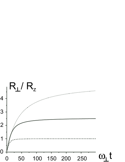
FIG. 1.: Aspect ratio as a function of the normalized time $\omega_{\perp}t$ for different collisional regimes (initial aspect ratio $\lambda=0.1$): collisionless (dashed line, $\tau_{0}\longrightarrow\infty$), intermediate collisional regime (solid line, $\omega_{\perp}\tau_{0}=0.1$), hydrodynamic regime (dotted line, $\tau_{0}\longrightarrow 0$).

Let us finally comment on the effect of quantum statistics on the calculation of the relaxation time. For a Bose gas at temperature above $T_{c}$ the problem has been investigated in [22] where it has been shown that statistical effects do not play a significant role. In contrast, the relaxation time in a harmonically trapped dilute Fermi gases has been shown to be strongly affected by Pauli blocking at low temperature [23]. The effects of collisions in a strongly interacting Fermi gas, including the unitarity limit, have been recently addressed in [24].

A Equations

We make the following ansatz for the non equilibrium distribution function: $f({\bf r},{\bf v},t)=\Gamma f_{0}({\bf R}(t),{\bf V}(t))$ with $R_{i}=r_{i}/b_{i}$, $V_{i}=(v_{i}-\dot{b}_{i}r_{i}/b_{i})\theta_{i}^{-1/2}$ and $\Gamma=\Pi_{j}b_{j}^{-1}\theta_{j}^{-1/2}$. The dependence on time is contained through the parameters $b_{i}$ and $\theta_{i}$. Following [14], we substitute this ansatz into Eq. (4) and use the equation for the equilibrium distribution $f_{0}$. We find

$$\dot{\Gamma}f_{0}+\Gamma\sum_{i}\bigg{\{}V_{i}\frac{\partial f_{0}}{\partial R_{i}}\bigg{(}\frac{\theta_{i}^{1/2}}{b_{i}}-\frac{1}{b_{i}\theta_{i}^{1/2}}\frac{1}{\Pi_{j}b_{j}}\bigg{)}$$ (A1)

$$-\frac{\partial f_{0}}{\partial V_{i}}\bigg{[}\frac{R_{i}}{\theta_{i}^{1/2}}\bigg{(}\ddot{b}_{i}+\omega_{i}^{2}b_{i}-\frac{\omega_{i}^{2}}{b_{i}}\frac{1}{\Pi_{j}b_{j}}\bigg{)}$$ (A2)

$$+V_{i}\bigg{(}\frac{1}{2}\frac{\dot{\theta}_{i}}{\theta_{i}}+\frac{\dot{b}_{i}}{b_{i}}\bigg{)}\bigg{]}\bigg{\}}=I_{\rm coll}$$ (A3)

Performing integration in phase space, we calculate the average moment of $R_{i}V_{i}$, namely $\int R_{i}V_{i}[Eq.(\ref{bs})]d^{3}Rd^{3}V/N$. This leads to Eq. (5). Note that this equation is not affected by the collision integral since the quantity $R_{i}V_{i}$ is conserved by collisions.

To derive Eq. (6), we consider instead the average moment of $V_{i}^{2}$. This yields:

$$\frac{\dot{\theta}_{i}}{\theta_{i}}+2\frac{\dot{b}_{i}}{b_{i}}=\frac{m}{N\Gamma k_{B}T_{0}}\int V_{i}^{2}I_{\rm coll}d^{3}Rd^{3}V,$$ (A4)

where $T_{0}$ is the equilibrium temperature. Differently from (5), Eq. (A4) depends explicitly on the collision integral . In order to calculate the r.h.s of Eq. (A4), we use the relaxation time approximation: $I=-(f-f_{\rm le})/\tau_{0}$. The first term gives: $\int V_{i}^{2}fd^{3}Rd^{3}V=N\Gamma k_{B}T_{0}/m$. To obtain a relation among the $\theta$ scaling parameters one uses the identity $\langle v^{2}\rangle=\langle v^{2}\rangle_{\rm le}$, from which we deduce $\bar{\theta}=\sum_{i}\theta_{i}/3$. The contribution of the local equilibrium term to the second term is obtained by noticing that, at local equilibrium, $\theta_{i}^{\rm le}=\bar{\theta}$: $\int V_{i}^{2}f_{\rm le}d^{3}Rd^{3}V=\bar{\Gamma}\int V_{i}^{2}f_{0}(\bar{{\bf R}},\bar{{\bf V}})d^{3}Rd^{3}V=N\Gamma\bar{\theta}k_{B}T_{0}/(m\theta_{i})$. Hence Eq. (A4) can be recast in the form (6).

REFERENCES

- [1] M.H. Anderson et al., Science 269, 198 (1995); K.B. Davis et al., Phys. Rev. Lett. 75 3969 (1995).
- [2] Y. Castin et al., Phys. Rev. Lett. 77, 5315 (1996); V.M. Perez-Garcia et al., Phys. Rev. Lett. 77, 5320 (1996); K.G. Singh et al. Rokhsar, Phys. Rev. Lett. 77, 1667 (1996); F. Dalfovo et al., Phys. Lett. A 227 259 (1997).
- [3] Yu. Kagan et al., Phys. Rev. A 55, R18 (1997).
- [4] C. Menotti et al., Phys. Rev. Lett. 89, 250402 (2002).
- [5] K.M. O’Hara et al., Science 298, 2179 (2002).
- [6] J. Cubizolles et al., cond-mat/0303079.
- [7] C.A. Regal and D.S. Jin, cond-mat/0302246.
- [8] D. M. Stamper-Kurn et al., Phys. Rev. Lett. 81, 500 (1998); M. Leduc et al., Acta Physica Polonica B 33, 2213 (2002); I. Shvarchuck et al., Phys. Rev. Lett. 89, 270404 (2002).
- [9] Private communications from J. Walraven (Amolf, Amsterdam), Zoran Hadzibabic (MIT, Cambridge), Fabrice Gerbier (IOTA, Orsay).
- [10] E. Zaremba et al., J. Low Temp. Phys. 116, 277 (1999).
- [11] For fermions, the density as well as the distribution function refers to a single species.
- [12] K. Huang, Statistical Mechanics, (J. Wiley, New York, 1987), 2nd ed.
- [13] L.P. Kadanoff and G. Baym, Quantum Statistical Mechanics (W.A. Benjamin, New York, 1962).
- [14] D. Guéry-Odelin, Phys. Rev. A 66, 033613 (2002).
- [15] We define as the average in position and velocity space of the function weighted by the equilibrium distribution function: .
- [16] L.P. Pitaevskii et al., Phys. Rev. A 55, R853 (1997).
- [17] D. Guéry-Odelin et al., Phys. Rev. A 60, 4851 (1999); U. Al Khawaja et al., J. Low Temp. Phys. 118, 127 (2000).
- [18] S. Stringari, Phys. Rev. Lett. 77, 2360 (1996).
- [19] H. Wu and E. Arimondo, Europhys. Lett. 43, 141 (1998).
- [20] In the unitary limit of -wave collisions, the cross section scales as where is the wave vector for the relative velocity which suggests a different scaling for given by .
- [21] Personal communication with J. Walraven.
- [22] G. M. Kavoulakis et al., Phys. Rev. A 61, 053603 (2000).
- [23] L. Vichi, J. Low. Temp. Phys. 121, 177 (2000).
- [24] M.E. Gehm et al., cond-mat/0304633.