Unrestricted Hartree-Fock for Quantum Dots

Abstract

We present detailed results of Unrestricted Hartree-Fock (UHF) calculations for up to eight electrons in a parabolic quantum dot. The UHF energies are shown to provide rather accurate estimates of the ground-state energy in the entire range of parameters from high densities with shell model characteristics to low densities with Wigner molecule features. To elucidate the significance of breaking the rotational symmetry, we compare Restricted Hartree-Fock (RHF) and UHF. While UHF symmetry breaking admits lower ground-state energies, misconceptions in the interpretation of UHF densities are pointed out. An analysis of the orbital energies shows that for very strong interaction the UHF Hamiltonian is equivalent to a tight-binding Hamiltonian. This explains why the UHF energies become nearly spin independent in this regime while the RHF energies do not. The UHF densities display an even-odd effect which is related to the angular momentum of the Wigner molecule. In a weak transversal magnetic field this even-odd effect disappears.

I Introduction

In the present work we discuss properties, predictions, and limitations of Hartree-Fock (HF) calculations for quantum dots. This method has a long tradition in atomic and nuclear physics, its application to quantum dots is therefore natural and has been discussed in various recent papers.Szafran et al. (2003); Sundqvist et al. (2002); Reusch et al. (2001); Yannouleas and Landman (1999); Müller and Koonin (1996); Fujito et al. (1996); Palacios et al. (1994); Pfannkuche et al. (1993) As we will demonstrate, some of the conclusions drawn on the basis of HF calculations are not based on firm grounds. This is in particular the case, when the HF wave functions are used to describe charge distributions in a quantum dot. On the other hand, Unrestricted Hartree-Fock (UHF) will be shown to give rather reliable estimates for the ground state energies.

While quantum dots may be considered as tunable artificial atoms, the electron density can be much smaller than in real atoms and correlations play a more prominent role.Reimann and Manninen (2002) This is why for quantum dots the HF method has to be regarded with care. In this work we focus on the crossover from weak to strong Coulomb interaction, i.e. from higher to lower electronic densities. This is equivalent to weakening the external confinement potential for a given host material of the quantum dot.

The physics of this crossover can be sketched as follows: In the case of weak interaction (high density) a one-particle picture is valid: Electrons are filled into the energy shells of the two dimensional isotropic harmonic oscillator. Here, the appropriate method is Restricted Hartree-Fock (RHF),Fujito et al. (1996); Pfannkuche et al. (1993) where every orbital belongs to an energetic shell and has good orbital momentum. This shell filling with Hund’s rule has been probed experimentally in small dots.Tarucha et al. (1996) In the case of strong interaction (low density) one can no longer stay within this simple one-particle picture: Wigner Wigner (1938) has shown that for strong correlation the ground state of the 2D electron gas is described by localized electrons, representing a classical hexagonal crystal. Accordingly, in this limit the electrons in the dot form a small crystal, a so-called Wigner molecule, and the picture of energetic shells is no longer meaningful. One has to improve the HF approximation by passing over to UHF which means that the space of the HF trial wave functions is extended. The UHF Slater determinant lowers the energy by breaking the symmetry of the problem, i.e. spatial and spin rotational invariance. This complicates the interpretation of the UHF solution.

For very strong interaction UHF is also expected to give reasonable results because a one-particle picture of localized orbitalsSundqvist et al. (2002) should model the Wigner molecule quite well. In fact, the UHF energies become nearly spin independent, while this is not the case with RHF. We show that the UHF Hamiltonian for strong interaction has the same spectrum as a tight-binding Hamiltonian of a particle hopping between the sites of a Wigner molecule. The hopping matrix elements and on-site energies can be extracted from the UHF orbital energies. The localization-delocalization transition has already been probed experimentally in larger quantum dots, Zhitenev et al. (1999) so Wigner molecule spectroscopy is within reach of current technology.

An incomplete account of our results has been presented in an earlier short communication.Reusch et al. (2001) Here, we discuss in detail the two-electron problem and present an elaborate analysis of the limit of strong interaction. In Sect. II we shortly recall the model and method. In Sect. III we obtain explicit results for quantum-dot Helium that already show many features of HF solutions for higher electron numbers presented in Sect. IV. In Sect. V we also discuss the effect of a magnetic field.

II Hamiltonian and Hartree-Fock approximation

In this work we follow the notation and method presented in our earlier articleReusch et al. (2001) for zero magnetic field. The Hamiltonian of an isotropic parabolic quantum dot with magnetic field reads (see e.g. Refs. Reimann and Manninen, 2002; Szafran et al., 2003; Sundqvist et al., 2002; Reimann et al., 2000; Hirose and Wingreen, 1999; Ruan et al., 1995; Häusler, 2000; Egger et al., 1999; Mikhailov, 2002; Reusch et al., 2001; Yannouleas and Landman, 1999; Müller and Koonin, 1996; Fujito et al., 1996; Palacios et al., 1994; Pfannkuche et al., 1993; Chan and Ruan, 2001; Ruan and Cheung, 1999; Ruan et al., 2000; Taut, 1993; MacDonald et al., 1993)

$$H=\sum_{i=1}^{N}\left\{\frac{1}{2m^{*}}[\bm{p}_{i}+e\bm{A}(\bm{r}_{i})]^{2}+\frac{m^{*}\omega^{2}}{2}\bm{r}_{i}^{2}\right\}+\sum_{i<j}\frac{e^{2}/\kappa}{|\bm{r}_{i}-\bm{r}_{j}|}$$ (1)

where the positions (momenta) of the electrons are denoted by $\bm{r}_{j}\;(\bm{p}_{j})$. The effective mass is $m^{*}$, and the dielectric constant is $\kappa$. The vector potential of a homogeneous magnetic field $\bm{B}$ orthogonal to the plane of the quantum dot in symmetric gauge reads $\bm{A}(\bm{r})=\frac{B}{2}(-y,x,0)$, and the corresponding cyclotron frequency is $\omega_{c}=eB/m^{*}$.

Now we can introduce oscillator units, and describe the system dimensionless: energies in units of $\hbar\omega_{\rm eff}=\hbar\sqrt{\omega^{2}+\omega_{c}^{2}/4}$ and lengths in units of $l_{0}=\sqrt{\hbar/m^{*}\omega_{\rm eff}}$. Then the Hamiltonian takes the form

$$H=\sum_{i=1}^{N}(-\frac{1}{2}\triangle_{i}+\frac{1}{2}\bm{r}_{i}^{2})-\frac{\omega_{c}}{2\omega_{\rm eff}}L_{z}^{\rm tot}+\sum_{i<j}\frac{\lambda}{|\bm{r}_{i}-\bm{r}_{j}|}\;,$$ (2)

where we have introduced the dimensionless coupling constant

$$\lambda=l_{0}/a^{*}_{\rm B}=e^{2}/\kappa l_{0}\hbar\omega$$ (3)

with the effective Bohr radius $a^{*}_{\rm B}$. For example $\lambda\!=\!2$ corresponds to $\hbar\omega\!\approx\!3$meV for a GaAs quantum dot. The Hamiltonian (2) is formally the same as without magnetic field, apart from an additional term proportional to the total angular momentum which scales with the dimensionless parameter foot6 $\Omega_{c}:=\omega_{c}/\omega_{\rm eff}$. The major part of our calculations presented below is for zero magnetic field.

Regarding the HF approximation,Fock (1930) let us recall the expansion of the HF orbitals in terms of the angular momentum eigenfunctions of the two-dimensional harmonic oscillatorReusch et al. (2001)

$$\langle\bm{r}|i\rangle=\varphi_{i}(\bm{r})=\sum_{\begin{subarray}{c}n=0,\infty\\ M=-\infty,\infty\end{subarray}}u_{nM}^{i}\langle\bm{r}|nM\sigma_{i}\rangle\;.$$ (4)

Here, $M$ is the angular and $n$ the radial quantum number of the Fock-Darwin basis. Each orbital has its own fixed spin $\sigma_{i}=\pm 1/2$, this means there is no double occupancy of orbitals with spin up and down, but there are different orbitals for different spins. Thus only the $z$-component of the total spin is fixed, $S_{z}^{\rm tot}=\sum_{i}\sigma_{i}\equiv S_{z}$. Furthermore, the orbitals (4) are in general no longer eigenfunctions of the one-particle angular momentum (UHF). Therefore the HF Slater determinant is not an eigenstate of the total angular momentum $L_{z}^{\rm tot}$, it breaks the symmetry of the original Hamiltonian.foot2 Another possibility is to give each orbital $i$ a fixed angular momentum $M_{i}$. With this restriction one obtains RHF Fujito et al. (1996); Pfannkuche et al. (1993) which preserves the total angular momentum but yields higher ground-state energies. Still another possibility is to build a Slater determinant of spatially localized orbitals for the strongly interacting caseSundqvist et al. (2002) or of multicenter localized orbitals in high magnetic fieldSzafran et al. (2003) and vary these orbitals to minimize the HF energy. Our orbitals are self-consistent and are best adapted to study the crossover from weak to strong correlation.

In principle the orientation of the deformed symmetry-breaking HF solution is arbitrary. This is due to the rotational invariance of the original Hamiltonian and can be called orientational degeneracy. The actual UHF solution found has a special orientation and it depends on the initial guess for the density matrix. Often but not always the symmetry breaking is manifested in the HF single-particle density $n^{\rm{HF}}(\bm{r})=\sum_{i=1}^{N}|\varphi_{i}(\bm{r})|^{2}$. For a quantum dot in zero magnetic field, the Hamiltonian is invariant under time reversal. Thus we can choose real expansion coefficients $u^{i}_{nM}$ in (4). However, then the HF one-particle density is always symmetric to one axis. Any arbitrary orientation can be obtained by applying $\exp(i\alpha L^{\rm tot}_{z})$ to the Slater determinant.

III Unrestricted Hartree-Fock for quantum-dot Helium

In this section we present UHF energies and densities for the two-electron quantum dot (quantum-dot Helium) at zero magnetic field for increasing interaction strength $\lambda$. This illustrates the basic concepts and properties of the HF approximation, and reveals features that are also important for higher electron numbers. We compare with exact results obtained by diagonalization of the relative motion. We also compare with the RHF method, in order to illustrate the differences to UHF.

The UHF two-electron problem has been treated previously by Yannouleas and Landman.Yannouleas and Landman (1999) However, we find some deviations from their results. An extensive discussion of the RHF solution for quantum-dot Helium at $\lambda\approx 2$ can be found in Ref. Pfannkuche et al., 1993. Finally, we want to mention that the two-electron problem has also an analytic solution in terms of a power series.Taut (1993)

III.1 Two-electron Slater determinant

The Slater determinant for two electrons with $S_{z}=0$ is

$$\Psi^{\rm{HF}}=\frac{1}{\sqrt{2}}\left[\varphi_{1}(\bm{r}_{1})\varphi_{2}(\bm{r}_{2})\chi_{+}^{1}\chi_{-}^{2}-\varphi_{1}(\bm{r}_{2})\varphi_{2}(\bm{r}_{1})\chi_{+}^{2}\chi_{-}^{1}\right].$$ (5)

Here we have displayed the orbital and spin parts of the wave function explicitly, $\chi_{\pm}^{i}$ is the spin of the $i$-th electron. The state $\Psi^{\rm{HF}}$ is generally not an eigenstate of the total spin $\bm{S}^{2}_{\rm tot}$. In order to obtain a singlet one has to set $\varphi_{1}\!=\!\varphi_{2}$, and thus

$$\Psi^{\rm{HF}}=\varphi_{1}(\bm{r}_{1})\varphi_{1}(\bm{r}_{2})\chi_{\rm singlet}.$$ (6)

This restriction is also called closed-shell HF (CSHF), because if every orbital is filled with spin up and down, open shells are impossible. One sees from (5) that the Slater determinant violates the symmetry of the problem. For two electrons the spin symmetry is easily restored, namely by a superposition of two Slater determinants with spin up/down and down/up. For the polarized case $S_{z}=1$, the total spin is conserved, and the HF wave function is a product of a symmetric spin function and an antisymmetric orbital function.

III.2 Different HF approximations

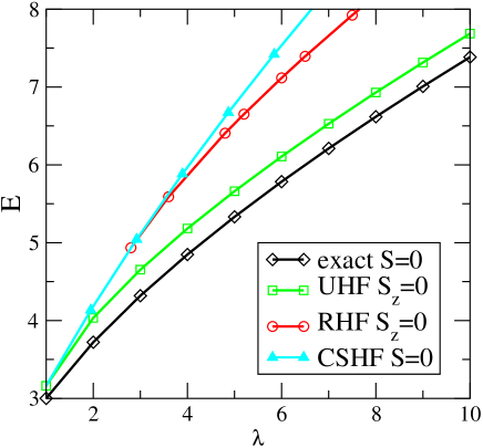
Figure 1: Comparison of different HF energies for quantum-dot Helium with the exact ground state energy vs. the coupling constant $\lambda$.

We now compare the energies of different HF approximations with the results of an exact diagonalization.Reusch et al. (2001) First we consider the case $S_{z}=0$. The most general ansatz for the HF orbitals is the UHF state (4), a spin dependent expansion with arbitrary angular momentum. Less general is the RHF ansatz, where angular momentum is preserved. And still less general is CSHF (6), when we force the two electrons to occupy two identical (rotationally symmetric) orbitals. In Fig. 1 one can clearly see the importance of breaking the symmetry to obtain lower HF energies. Up to $\lambda\approx 1$ all three methods give nearly the same result. Up to $\lambda\approx 3$ the closed-shell energy is equal to the RHF energy. In other words: From this point on the two RHF orbitals are no longer identical. As expected the UHF energy is lowest.

In Fig. 2 we show the differences of the RHF and UHF energies from the energy of the exact ground state which is the singlet. For $S_{z}=1$ one needs two different orbitals, there is no CSHF. The UHF method gives lower energies than RHF, but the gain in energy is not as big as in the unpolarized case. Interestingly, the UHF energies become spin independent with increasing $\lambda$: they agree within about $0.3\%$, the $S_{z}=1$ state is somewhat lower than the $S_{z}=0$ state.

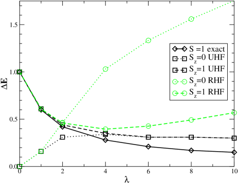
Figure 2: Absolute energy differences with respect to the exact $S=0$ ground state $\Delta E=E_{S}-E_{\rm GS}^{\rm exact}$. Above $\lambda\approx 4$ the two UHF energies are nearly the same.

The exact energies merge more slowly: for $\lambda=20$ the energy difference between singlet and triplet is still about $1\%$. Note that the RHF energies fail to become spin independent for large $\lambda$, as can be seen from Fig. 2. Of course, one expects spin independent energies in the classical limit of localized electrons without overlap.

III.3 UHF one-particle densities

Now we want to have a closer look at the one-particle density which is just the sum of the densities of the two orbitals, $n^{\rm{HF}}(\bm{r})=|\varphi_{1}(\bm{r})|^{2}+|\varphi_{2}(\bm{r})|^{2}$.

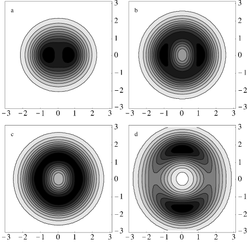
Figure 3: Shadowed contour plots of the UHF one-particle densities $n^{\rm{HF}}$ for $N=2$, $S_{z}=0$. One contour corresponds to $1/10$ of the maximal density. (a) $\lambda=2$, (b) $\lambda=6$, (c) $\lambda=8$, (d) $\lambda=20$.

In Figs. 3 and 4 we show this density for different values of the coupling parameter $\lambda$. Already for a relatively small $\lambda$ we detect two azimuthal maxima. The density is strongly anisotropic which is due to the symmetry breaking. In the case of $S_{z}=1$ the two maxima are more distinct as a consequence of the Pauli principle: spin-polarized electrons are more strongly correlated. However, the direct interpretation of the two dips as localized electrons is questionable. With increasing $\lambda$ the azimuthal modulation first decreases, but for $\lambda\gtrsim 8$ ( $\lambda\gtrsim 10$ for $S_{z}=1$) it increases again. For very high $\lambda$ the densities become almost spin independent.

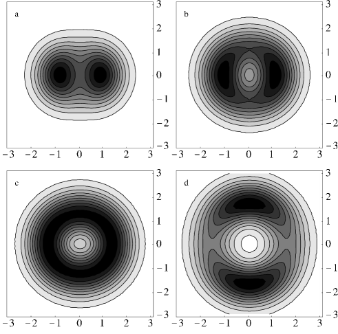
Figure 4: UHF one-particle densities for $N=2$, $S_{z}=1$. (a) $\lambda=2$, (b) $\lambda=6$, (c) $\lambda=8$, (d) $\lambda=20$.

A closer view reveals that the azimuthal maxima are more distinct for the case $S_{z}=0$. This arises from the exchange term in the HF energy: it lowers the energy for strong interaction and overlapping spin-polarized orbitals.

While the azimuthal modulation is an artifact of the HF method, the densities display correctly a minimum in the center which gets deeper with stronger interaction. Also, the maxima are in very good agreement with the classical positions $r_{a}=\sqrt[3]{\lambda/4}$ (see Appendix A).

III.4 UHF orbitals and orbital energies

In order to understand the form of the UHF densities it is useful to have a closer look at the UHF orbitals. For $S_{z}=0$ we find two orbitals that are exactly complex conjugate, $\varphi_{1}=\varphi_{2}^{*}$. This can be seen by studying the expansion coefficients $u_{nM}$ in Eq. (4) and means that the Slater determinant is symmetric under time reversal.

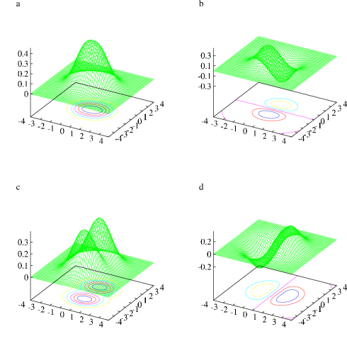
Figure 5: Pairs of real UHF orbitals for $N=2$, $S_{z}=1$. (a), (b) at $\lambda=2$, (c), (d) at $\lambda=10$.

For $S_{z}=1$ the two orbitals depicted in Fig. 5 are always different and can be chosen real. For $\lambda=2$ one can still interpret the orbitals in the energy shell picture of RHF: the first orbital is (approximately) round, S-like, and the second one is dumbbell formed, P-like.foot2

For very high $\lambda\gtrsim 14$ there is a simple relation between the orbitals for the two spin polarizations: for $S_{z}=1$ we may choose both orbitals real and then we find

$$\varphi_{1/2}^{S=0}\approx\frac{1}{\sqrt{2}}(\varphi_{1}^{S=1}\pm i\varphi_{2}^{S=1})\;.$$ (7)

In this fashion, we see that $\varphi_{1/2}^{S=0}$ are complex conjugate and approximately orthonormal.

To shed more light on this behavior we consider also the orbital energies. We start with the HF Hamiltonian in the HF basis for $S_{z}=1$

$$\left(\begin{array}[]{cc}\varepsilon_{1}&0\\ 0&\varepsilon_{2}\\ \end{array}\right)=\left(\begin{array}[]{cc}h_{11}+w_{1212}&0\\ 0&h_{22}+w_{1212}\\ \end{array}\right)\;.$$ (8)

Here, we use the notation $h_{ij}=\left\langle i\right|h\left|j\right\rangle$ and $w_{ijkl}=(ij|w|kl)$ for matrix elements in the HF basis (see Ref. Reusch et al., 2001). When we apply the unitary transform (7)

$$\frac{1}{2}\left(\begin{array}[]{rr}1&i\\ 1&-i\\ \end{array}\right)\left(\begin{array}[]{cc}\varepsilon_{1}&0\\ 0&\varepsilon_{2}\\ \end{array}\right)\left(\begin{array}[]{rr}1&1\\ -i&i\\ \end{array}\right)=\left(\begin{array}[]{rr}U&-t\\ -t&U\\ \end{array}\right)=H_{2}\;$$ (9)

we obtain a two-state Hamiltonian $H_{2}$, with on-site energy $U\!=\!(h_{11}+h_{22}+2w_{1212})/2$ and tunnel splitting $t\!=\!(h_{22}-h_{11})/2$. Thereby, we have mapped the HF Hamiltonian on a lattice problem.It is intuitive that for strong interaction the two electrons localize, and thus a tight-binding approach should become physically correct. This is also the case for larger electron number as discussed below.

III.5 UHF two-particle densities

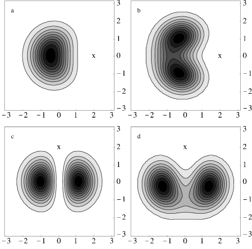
Figure 6: UHF Conditional probability density $n^{\rm{HF}}(\bm{x}|\bm{y})$ for $N=2$, $S_{z}=1$. In the upper row $\bm{y}=(2,0)$ (x) (a) $\lambda=2$, (b) $\lambda=6$. Lower row $\bm{y}=(0,2)$ (x) (c) $\lambda=2$, (d) $\lambda=10$.

Next we examine the conditional probability density (CPD) for finding one electron at $\bm{x}$, under the condition that another electron is at $\bm{y}$. For quantum-dot Helium and $S_{z}=0$ the CPD reads

$$n^{\rm{HF}}(\bm{x}|\bm{y})=\frac{|\varphi_{1}(\bm{x})|^{2}|\varphi_{2}(\bm{y})|^{2}+|\varphi_{1}(\bm{y})|^{2}|\varphi_{2}(\bm{x})|^{2}}{n^{\rm{HF}}(\bm{y})}\;.$$ (10)

Now, since we found complex conjugate orbitals, $\varphi_{1}=\varphi_{2}^{*}$, we have $n^{\rm{HF}}(\bm{x}|\bm{y})=n^{\rm{HF}}(\bm{x})$, i.e. the conditional probability density is independent of the condition. This is not really astonishing, because within the HF method two electrons are only correlated by the exchange term, which vanishes here. foot2a

For $S_{z}=1$ the orbitals are different from each other and the CPD is given by

$$n^{\rm{HF}}(\bm{x}|\bm{y})=\{|\varphi_{1}(\bm{x})|^{2}|\varphi_{2}(\bm{y})|^{2}+|\varphi_{1}(\bm{y})|^{2}|\varphi_{2}(\bm{x})|^{2}$$

$$-2{\rm Re}[\varphi_{1}^{*}(\bm{x})\varphi_{2}(\bm{x})\varphi_{1}(\bm{y})\varphi_{2}^{*}(\bm{y})]\}/n^{\rm{HF}}(\bm{y})\;.\;$$ (11)

In Fig. 6 we show contour plots of UHF CPDs for different coupling constants and given positions $\bm{y}$. In the upper row, for $\bm{y}=(2,0)$, we find for small $\lambda=2$ a suggestive result: the density has a single maximum at a distinct distance from the fixed coordinate $\bm{y}$. With increasing $\lambda$, however, we obtain two maxima, which develop more and more and are not at all located at the classical position.

The situation is likewise irritating when one chooses $\bm{y}=(0,2)$ as fixed coordinate (lower row). While the exact CPD is rotationally symmetric when both $\bm{x}$ and $\bm{y}$ are rotated, the UHF CPD does not respect this symmetry. The reason for this lies in the symmetry breaking which cannot completely account for correlations. The UHF Slater determinant is deformed and derived quantities do not necessarily have a direct physical meaning, – except for the UHF energy which is a true upper bound for the exact energy.

IV Unrestricted Hartree-Fock for higher electron numbers

In this section we show further results of UHF calculations, namely energies and densities for up to eight electrons ($B=0$). Many effects are similar to what we have already seen for two electrons, for example the errors of the UHF energies and their spin dependence. An interesting phenomenon shown by the UHF densities is the even-odd effect discussed below.

IV.1 UHF energies

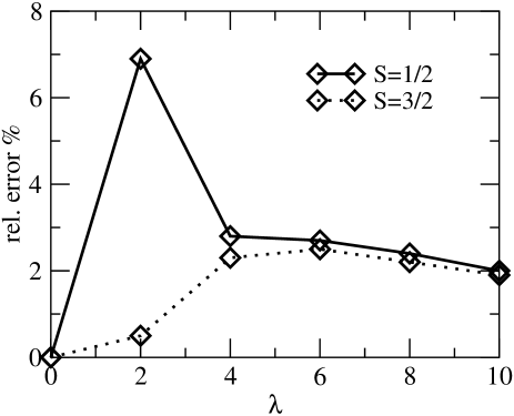
Figure 7: Relative error of the UHF energy $(E_{S}^{\rm{HF}}-E_{S}^{\rm QMC})/E_{S}^{\rm QMC}$ for $N=3$ vs. coupling constant $\lambda$.

For $N>2$ we compare the UHF energies with results of a Quantum Monte Carlo (QMC) simulation by Egger et al.Egger et al. (1999) These results were obtained for a very low temperature $T\!=\!0.1\hbar\omega/k_{\rm B}$. The QMC energies are always below the HF energies and can therefore be considered as effective zero temperature reference points.

For $N=3$ QMC, a semiclassical analysis, Häusler (2000) as well as an exact diagonalization study Mikhailov (2002) predict a transition from the $S=1/2$ ground state in the weakly interacting case to a $S=3/2$ ground state for $\lambda\gtrsim 4$. Within UHF this transition occurs already near $\lambda=2$. In Fig. 7 one can see that the relative error for $S_{z}=3/2$ is small, less than 3% . In the non-polarized case the error is higher, about  7% for $\lambda\gtrsim 2$. With increasing $N$ and $\lambda$ the relative error becomes smaller because the absolute energies are higher.

In Fig. 8 we show the absolute energy differences from the QMC ground state for eight electrons. For intermediate values of $\lambda$ the UHF energies become already nearly spin independent, whereas the QMC energies approach this semiclassical behavior more slowly. For stronger interaction the HF ground state is always spin-polarized. Thus the UHF method can not resolve the correct spin ordering of the energies.

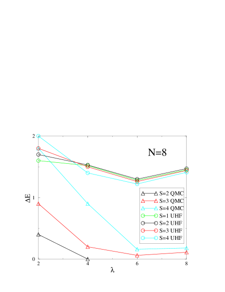
Figure 8: Absolute energy differences from the QMC ground state, $\Delta E=E_{S}-E_{\rm GS}^{\rm QMC}$ for eight electrons and various spins vs. coupling constant $\lambda$.

For $N\!=\!8$ the QMC method predicts a crossover of the total spin from $S\!=\!1$ to $S\!=\!2$ near $\lambda=4$. The UHF method finds a polarized ground state with $S\!=\!4$ for $\lambda\gtrsim 4$. There, however, the energy differences for different spins are already quite small.

One can conclude that the UHF Slater determinant with fixed spin structure gives a rather poor description of the total many-electron wave function. Essentially, UHF renders the properties of the spin-polarized solution for larger $\lambda$. This can also be seen in the UHF densities, which become spin independent for larger interaction (see below). Finally, we briefly mention the RHF results: there for large $\lambda$ the HF energies do not become spin independent, but the energies for lower spins are considerably higher. For large $\lambda$ RHF gives a poor estimate of the ground state energy.

IV.2 HF densities: Even-odd effect

In this subsection we consider the UHF densities for higher electron numbers. We first show in Fig. 9 the densities for rather strong coupling constant  $\lambda=6$, various electron numbers $N$ and $S_{z}=N/2$. Above this interaction strength the UHF densities are essentially the same for all $S_{z}$ (except for $N=2$, see above) and do not change qualitatively with increasing $\lambda$.

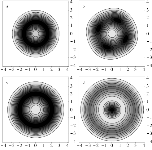
Figure 9: Even-odd effect of the UHF one-particle densities  $n^{\rm{HF}}$ for $\lambda=6$, different electron numbers $N$ and polarized spin $S_{z}=N/2$. (a) $N=3$, (b) $N=4$, (c) $N=5$, (d) $N=8$.

Surprisingly, only for some $N$ does one obtain a molecule-like structure, i.e. an azimuthal modulation as seen for two electrons. For three and five electrons the density is apparently rotationally symmetric and also for eight electrons, where we have a pronounced maximum in the center. The expected molecule-like structure shows up only for $N=2$ and 4. Thus, when we consider also $N=6,7$ (see below) we recognize that azimuthal maxima occur only for an even number of electrons per spatial shell. In stating this we want to emphasize, that all the densities shown belong to symmetry breaking, deformed Slater determinants.

This even-odd effect is also surprising, because UHF calculations for quantum dots in a strong magnetic field Müller and Koonin (1996) found molecule-like densities for all electron numbers, and frequently a magnetic field leads to similar effects as a stronger interaction. We also have performed calculations with a magnetic field that reproduce the densities of Ref. Müller and Koonin, 1996 and show that the molecule-like structure disappears for odd $N$ for vanishing field. foot3

A physical explanation of the even-odd effect combines the geometry of the classical system with the symmetry of quantum mechanics. Ruan et al. (1995) Consider the exact spin-polarized $N$-electron wave function $\Psi_{N}$ for the Wigner molecule case. Due to the strong Coulomb repulsion, the electrons move on an $N$-fold equilateral polygon (for $N<6$; for $N=6$ one electron enters the center of the dot). A rotation by $2\pi/N$ therefore corresponds to a cyclic permutation

$$\exp\left\{\frac{2\pi i}{N}\;L^{\rm tot}_{z}\right\}\;\Psi_{N}=(-1)^{N-1}\;\Psi_{N}\;,$$ (12)

where we have used that a cyclic permutation of an even (odd) number of electrons is odd (even). From Eq. (12) the allowed total angular momenta of the Wigner molecule can be easily read off: for an odd number of electrons the minimal angular momentum is zero, whereas it is nonzero and degenerate for an even electron number, e.g. $M^{\rm tot}=\pm 2$ for $N=4$. Hence, the UHF wave functions for $N=2,4,7$ can be interpreted as standing waves, i.e. superpositions of opposite angular momentum states. For odd numbers of electrons in a spatial shell there is no angular momentum degeneracy and therefore no standing wave and no modulation in the densities. With a similar argument Hirose and Wingreen Hirose and Wingreen (1999) explain the charge-density-waves which they found for odd number of electrons in the weakly interacting regime from density functional calculations.

Equation (12) does not hold anymore when the spins are not polarized, because the total wave function is not a product of spin and orbital wave functions. However, within UHF we do not fix the exact spin but only subspaces with fixed $S_{z}$. For $S_{z}<N/2$ and strong interaction the UHF solution mainly renders the properties of the spin-polarized solution, since the energies and densities are essentially the same for $\lambda\gtrsim 6$. The even-odd effect is thus not a physical effect but an artifact of the UHF symmetry breaking. Therefore great caution must be taken when interpreting the UHF densities. In particular, the exact onset of Wigner crystallization cannot be determined reliably from UHF calculations.

IV.3 Closer look at three electrons

As we have just discussed, for three electrons with strong interaction we do not find the naively expected density with three maxima but a nearly round density. When we plot the density of Fig. 9(a) with more contour lines (not shown) a tiny sixfold modulation of the density is discernible. This can be understood by going back to Eq. (12): after $M^{\rm tot}=0$ the next allowed total angular momentum values are $M^{\rm tot}=\pm 3$, which give rise to a standing wave with six maxima. This becomes also clear from the densities of the single orbitals building the UHF single-particle density.

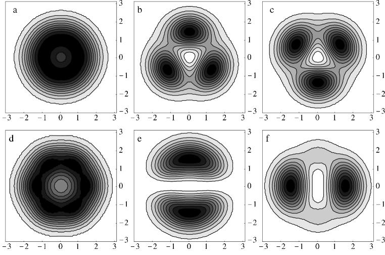
Figure 10: UHF orbital densities $|\varphi_{i}|^{2}$ ($i=1,2,3$) for $N=3$ and $S_{z}=3/2$. Upper row $\lambda=4$, lower row $\lambda=6$. For the single-particle energies we obtain (a) $\varepsilon_{1}=4.92$ and (b), (c) $\varepsilon_{2}=\varepsilon_{3}=5.84$; (d) $\varepsilon_{1}=6.44$ and (e), (f) $\varepsilon_{2}=\varepsilon_{3}=7.11$.

In Fig. 10 we show the orbital densities for $\lambda=4$ and $\lambda=6$. We find a sixfold orbital, as well as two diametrically oriented threefold orbitals. One clearly recognizes how the sixfold modulation results from this. Note that the HF orbitals are not localized (for example at the angles of a triangle).

At this point we want to address a related issue, the uniqueness of the HF orbitals. One can easily show with the help of the HF equations that HF orbitals with the same spin are no longer unique, if the corresponding one-particle energies $\varepsilon_{i}$ are degenerate. In this case, any unitary transformation of degenerate orbitals also fulfills the HF equations. In Fig. 10, the energies $\varepsilon_{i}$ are degenerate for the two states (b),(c) and (e),(f). Therefore these two orbitals are no longer uniquely determined, – in addition to the orientational degeneracy of the total Slater determinant  which is physically obvious.

Now, we want to have a closer look on the orbital energies: it is natural to presume that their degeneracies are a signature of Wigner crystallization, i.e. the geometry of the Wigner molecule. For strong interaction one should be able to represent the system as a lattice problem on an equilateral triangle. The corresponding Hamiltonian for $N=3$, $S_{z}=3/2$ reads

$$H_{3}=\left(\begin{array}[]{rrr}U&-t&-t\\ -t&U&-t\\ -t&-t&U\end{array}\right)\;,$$ (13)

where $U$ is the on-site energy and $t$ is the tunneling matrix element between localized states. The eigenvalues of $H_{3}$ are $\varepsilon_{1}=U-2t$ and twice $\varepsilon_{2/3}=U+t$ which is in fact the degeneracy of the UHF orbital energies (Fig. 10).

On the other hand, for $S_{z}=1/2$ the tight-binding Hamiltonian involves tunneling only between the two spin up states and takes the form

$$H_{3}^{\prime}=\left(\begin{array}[]{rrc}U&-t&0\\ -t&U&0\\ 0&0&U\end{array}\right)\;.$$ (14)

The eigenvalues are $\varepsilon_{1/2}=U\pm t$ (spin up) and $\varepsilon_{3}=U$ (spin down). With UHF for $\lambda=6$ we find $\varepsilon_{1}=6.65$, $\varepsilon_{2}=7.10$ and $\varepsilon_{3}=6.87$, which has to be compared with the orbital energies for the polarized state given in Fig. 10 and yields $t\approx 0.22$. For larger $\lambda$ the agreement becomes better, e.g. for $\lambda=12$ we find $\varepsilon_{1}=10.140$, $\varepsilon_{2}=10.309$ and $\varepsilon_{3}=10.224$ for $S_{z}=1/2$, while $\varepsilon_{1}=10.06$ and $\varepsilon_{2/3}=10.313$ for $S_{z}=3/2$, which gives $t\approx 0.084$ in both cases.

IV.4 Lattice Hamiltonian and localized orbitals

For large $\lambda$ the HF Hamiltonian has the same eigenvalues as a lattice Hamiltonian. Thus, there must be one-to-one correspondence between these two. Remember, however, that HF is a one-particle picture and thus the tight binding Hamiltonian describes one particle hopping on a grid. The HF Hamiltonian is diagonal in the HF basis (4),

$$\left\langle i\right|h\left|j\right\rangle+\sum_{k}^{N}(ik|w|jk)=\varepsilon_{i}\delta_{ij}\;.$$ (15)

Now, if the eigenvalues $\varepsilon_{i}$ coincide with those of a lattice Hamiltonian, e.g. $H_{3}$ in (13), this means that we have to transform the UHF orbitals with the inverse of the orthogonal transformation which diagonalizes the lattice Hamiltonian to pass over to localized orbitals. The Slater determinant is not changed when we transform among occupied orbitals, Edmindston and Ruedenberg (1963)

$$\left|p\right\rangle=\sum_{i}^{N}o_{p}^{i}\left|i\right\rangle\;.$$ (16)

In this new basis the HF equations read

$$\sum_{q}^{N}\big{\{}\left\langle p\right|h\left|q\right\rangle+\sum_{r}^{N}(pr|w|qr)\big{\}}o^{i}_{q}=\varepsilon_{i}o^{i}_{p}\;.$$ (17)

Now, in the basis $\left|p\right\rangle$, we should have non vanishing $\left\langle p\right|h\left|q\right\rangle$ only for nearest neighbors foot4 and the contribution of the two-particle matrix element should essentially be given by the direct term, i.e. diagonal elements of the Coulomb interaction. Then (17) reduces to

$$\sum_{q}^{N}\big{\{}\left\langle p\right|h\left|q\right\rangle+\delta_{pq}\sum_{r}^{N}(pr|w|pr)\big{\}}o^{i}_{q}=\varepsilon_{i}o^{i}_{p}\;,$$ (18)

which is now of the form of a lattice Hamiltonian.

We now present strong numerical evidence for this connection between the UHF Hamiltonian and a lattice Hamiltonian for $N=4$ and 5 which are the simplest cases of electrons on a ring. For $N=4$, $S_{z}=2$ we have

$$H_{4}=\left(\begin{array}[]{rrrr}U&-t&0&-t\\ -t&U&-t&0\\ 0&-t&U&-t\\ -t&0&-t&U\end{array}\right)\;,$$ (19)

with the eigenvalues $\varepsilon_{1}=U-2t$, $\varepsilon_{2/3}=U$ and $\varepsilon_{4}=U+2t$. The eigenvectors of $H_{4}$ determine the transformation (16). Applying this transformation to the HF Hamiltonian, as we did in (9), we obtain for $\lambda=8$ an Hamiltonian of the form (19) with $U=10.924$ and $t=0.195$. The next nearest neighbor hopping matrix element (hopping along the diagonal of the square) is $t^{*}=2\varepsilon_{2}-\varepsilon_{1}-\varepsilon_{4}=0.003$, which is indeed very small.

Likewise we can determine the lattice Hamiltonians for other electron numbers and spin configurations and we have collected results for $t$ and $U$ for stronger interaction up to $\lambda=20$. For $N=4$, $S_{z}=1$ the lattice Hamiltonian reads

$$H_{4}^{\prime}=\left(\begin{array}[]{rrrc}U&-t&0&0\\ -t&U&-t&0\\ 0&-t&U&0\\ 0&0&0&\,U\end{array}\right)\;,$$ (20)

with the eigenvalues $\varepsilon_{1}=U-\sqrt{2}t$, $\varepsilon_{2}=U$ and $\varepsilon_{3}=U+\sqrt{2}t$ (spin up) and $\varepsilon_{4}=U$ (spin down), while for $N=4$, $S_{z}=0$ we have

$$H_{4}^{\prime\prime}=\left(\begin{array}[]{rrrr}U&-t&0&0\\ -t&U&0&0\\ 0&0&U&-t\\ 0&0&-t&U\end{array}\right)\;,$$ (21)

with $\varepsilon_{1/2}=U\pm t$ (spin up), $\varepsilon_{3/4}=U\pm t$ (spin down). Here, we have to assume that the four states are occupied with two pairs of nearest neighbor parallel spins in order to obtain agreement with the UHF orbital energies. The values of $t$ we obtain in this way for the three spin states $S_{z}=0,1,2$ agree within 1% for $\lambda=8$ .

For $N=5$ we have a pentagon and again three different spin states. For $S_{z}=5/2$ the lattice Hamiltonian with nearest neighbor hopping is

$$H_{5}=\left(\begin{array}[]{rrrrr}U&-t&0&0&-t\\ -t&U&-t&0&0\\ 0&-t&U&-t&0\\ 0&0&-t&U&-t\\ -t&0&0&-t&U\end{array}\right)\;,$$ (22)

with the eigenvalues $\varepsilon_{1}=U-2t$, $\varepsilon_{2/3}=U+t(1-\sqrt{5})/2$ and $\varepsilon_{4/5}=U+t(1+\sqrt{5})/2$, while for $S_{z}=3/2$ we have

$$H_{5}^{\prime}=\left(\begin{array}[]{rrrrc}U&-t&0&0&0\\ -t&U&-t&0&0\\ 0&-t&U&-t&0\\ 0&0&-t&U&0\\ 0&0&0&0&\,U\end{array}\right)\;,$$ (23)

with $\varepsilon_{1/2}=U-t(\sqrt{5}\pm 1)/2$, $\varepsilon_{3/4}=U+t(\sqrt{5}\mp 1)/2$ (spin up) and $\varepsilon_{5}=U$ (spin down). Finally for $S_{z}=1/2$ we have

$$H_{5}^{\prime\prime}=\left(\begin{array}[]{rrrcc}U&0&0&0&0\\ 0&U&-t&0&0\\ 0&-t&U&0&0\\ 0&0&0&\,U&0\\ 0&0&0&0&\,U\end{array}\right)\;,$$ (24)

with the eigenvalues $\varepsilon_{1/3}=U\pm t$, $\varepsilon_{2}=U$ (spin up) and $\varepsilon_{4/5}=U$ (spin down). Note that here the values of the UHF orbital energies suggest a model with only two nearest neighbor parallel spins. For $\lambda=6$ the values of $t$ for all three spin states coincide within 1%.

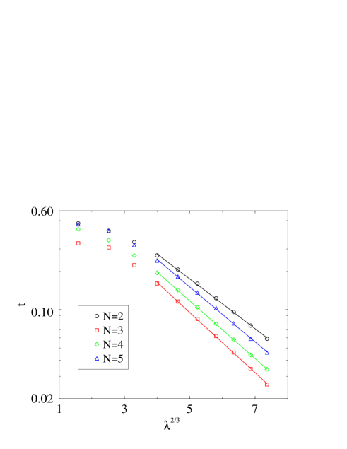
Figure 11: Log-linear plot of tunnel matrix element $t$ vs. $\lambda^{2/3}$ for various electron numbers. For $\lambda\geq 8$ the line of best fit is shown.

Figure 11 summarizes our findings about the tunnel matrix elements. Reference Häusler, 2000 predicts $t\propto\exp(-\sqrt{r_{s}})$, where $r_{s}$ is the nearest neighbor distance of the electrons measured in units of the effective Bohr radius. Since classically $r_{s}\propto\lambda^{4/3}$ (cf. Appendix A) we plot $\ln t$ versus $\lambda^{2/3}$. For $\lambda\gtrsim 8$ we find indeed a linear behavior. For lower $\lambda$, the tunneling matrix element is not really defined, since the lattice model is not appropriate. The tunneling matrix element is largest for $N=2$ because two electrons are always closest (see Appendix A). Three electrons always have the smallest value of $t$ because the corresponding equilateral triangle has a longer side than the square and the pentagon. For higher electron numbers one electron enters the center of the dot, and the UHF spectra are more complicate but still show the typical degeneracies. However, now the lattice Hamiltonian has various tunneling constants and on-site energies.

IV.5 Seven-electron Wigner molecule

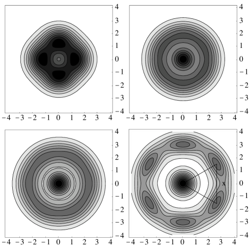
Figure 12: One-particle densities for the UHF ground state of $N=7$ electrons. (a) $\lambda=1$, (b) $\lambda=2$, both $S_{z}=1/2$. (c) $\lambda=4$, (d) $\lambda=10$, both $S_{z}=7/2$.

Seven classical electrons form a equilateral hexagon with one central electron, which is a fragment of a hexagonal lattice. In Fig. 12 we show UHF densities for $N=7$ starting with a small $\lambda$. The UHF ground state is $S_{z}=1/2$ up to $\lambda\lesssim 3$, then spin-polarized. In Fig. 12(a) for $\lambda=1$ we see a fourfold modulated density. How is that possible for seven electrons? The answer is that in this case the energy shell picture of the harmonic oscillator is still valid: six electrons are just a shell closure and the next electron is put in the new shell in an orbital with maximal angular momentum. This angular momentum is $M=\pm 2$ and from the superposition one obtains a fourfold standing wave (cf. Ref. Hirose and Wingreen, 1999). Here, the energy is basically the same as in RHF, but the Slater determinant breaks the symmetry.

With increasing interaction strength a Wigner molecule is formed with one electron in the center and six in the surrounding ring [Fig. 12(b)-(c)]. We want to emphasize that the UHF densities mirror the classical shell filling. This can even be quantified: the positions of the maxima (even in the ’round’ densities) agree very well with the classical configurations in Appendix A. From the UHF density the nearest neighbor distance $\tilde{r}_{s}$ can be determined. For example from Fig. 12(d) we find $\tilde{r}_{s}\approx 3.0$, which is also the classical value. Here we have to take into account that we measure length in oscillator units. Frequently, one is interested in the density parameter $r_{s}$ given in effective Bohr radii. foot5 Then Fig. 12(d) gives $r_{s}=\tilde{r}_{s}l_{0}/a^{*}_{\rm B}=\lambda\tilde{r}_{s}\approx 30$. The $r_{s}$ values we obtain in this way agree also well with the results of Ref. Egger et al., 1999. There $r_{s}$ is determined from the first maximum of the two-particle correlation function.

V Unrestricted Hartree-Fock with a magnetic field

In this section we want to present some calculations with a magnetic field orthogonal to the plane of the quantum dot. This system has been discussed extensively in the literature, especially in connection with the quantum Hall effect. UHF calculations by Müller and Koonin Müller and Koonin (1996) have shown a magnetic field induced Wigner crystallization. However, they only considered the limiting case of a strong magnetic field and therefore included in the basis for expanding the UHF orbitals only states from the lowest Landau level (Fock-Darwin levels with $n=0$). The high field case has also been studied by Palacios et al.Palacios et al. (1994) and Ruan et al.Chan and Ruan (2001); Ruan et al. (2000); Ruan and Cheung (1999) To study smaller magnetic fields, our basis is better adjusted to the problem. It is intuitively clear, that electrons are further localized by the magnetic field. Indeed, for sufficiently strong fields, we do not find an even-odd effect for UHF densities but molecule-like densities for all electron numbers.

Numerically, thanks to the similar form of the Hamiltonian (2) to the one without magnetic field, the generalization of our UHF code is straightforward. However, the magnetic field breaks time reversal symmetry, left and right turning solutions are no longer energetically degenerate. Therefore in the expansion of the UHF orbitals (4) we have to use complex coefficients.

We first consider three electrons and a large interaction parameter $\lambda=10$. This means that we have a shallow quantum dot where the Coulomb interaction dominates and the magnetic field is relatively weak. In Fig. 13 we display the evolution of the UHF one-particle densities with increasing magnetic field strength $\tilde{\omega}_{c}=\omega_{c}/\omega$ at fixed $\lambda$. This is not exactly the physical situation, corresponding to a quantum dot exposed to an increasing magnetic field, since the coupling constant $\lambda$ becomes smaller with increasing field. Here we just want to show that a magnetic field does not have the same effect on the UHF density as a strong interaction.

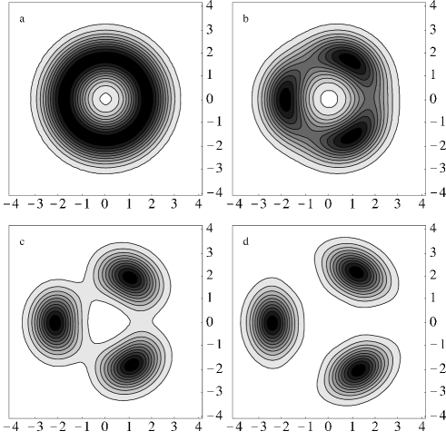
Figure 13: Evolution of the UHF one-particle densities for $N=3$, $S_{z}=3/2$ and $\lambda=10$ with increasing magnetic field strength $\tilde{\omega}_{c}=\omega_{c}/\omega$. (a) $\tilde{\omega}_{c}=0$, (b) $\tilde{\omega}_{c}=0.5$, (c) $\tilde{\omega}_{c}=1.5$, (d) $\tilde{\omega}_{c}=2.5$.

In Fig. 13(d) we see three distinct, localized electrons in the UHF density. The three single orbital densities have nearly the same form. They are thus similar to the orbitals chosen in Ref. Szafran et al., 2003. With decreasing magnetic field strength the maxima in azimuthal direction vanish slowly, until we have again a nearly round density for $\omega_{c}=0$ as in Fig. 9(a). The density in Fig. 13(a) has been obtained from an initial guess with threefold symmetry. Therefore we can be sure that we have not obtained a local minimum but the true HF ground state.

As a second example we show the evolution of the UHF density of six electrons at intermediate coupling strength $\lambda=3.2$. Without magnetic field the density is round, Fig. 14(a), and with a weak magnetic field fivefold with a central electron, Figs. 14(b),(c).

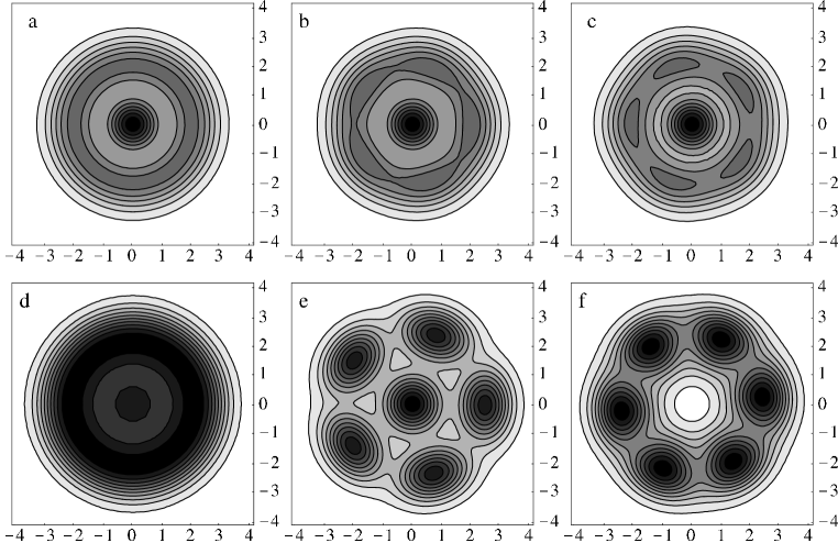
Figure 14: Evolution of the UHF one-particle density for $N=6$, $S_{z}=3$ and $\lambda=3.2$ with increasing magnetic field strength, (a) $\tilde{\omega}_{c}=0$, (b) $\tilde{\omega}_{c}=0.1$, (c) $\tilde{\omega}_{c}=0.5$, (d) $\tilde{\omega}_{c}=1$, (e) $\tilde{\omega}_{c}=2$, (f) $\tilde{\omega}_{c}=2.5$. In (f) sixfold isomer with energy $E^{*}_{\rm{HF}}=45.182$.

Remarkably, for intermediate magnetic field $\tilde{\omega}_{c}\approx 1\ldots 1.5$, the UHF ground state has a perfectly round density, Fig. 14(d), and also a rotationally symmetric Slater determinant. This is the so-called maximum-density-droplet of MacDonald et al.,MacDonald et al. (1993) where the electrons occupy the lowest orbitals with increasing angular momentum. Here the orbitals with $M=0$,1,2,3,4,5 are occupied, and the UHF solution is identical to the RHF solution with total angular momentum $M^{\rm tot}=15$.

Finally, in Fig. 14(e) for strong magnetic field we have a distinctly localized fivefold Wigner molecule. Figure 14(f) for $\tilde{\omega}_{c}=2.5$ shows a sixfold isomer which is higher in energy by 0.009 than the fivefold ground state.

VI Conclusion

In conclusion, we have discussed the properties of unrestricted Hartree-Fock (UHF) calculations for electrons in a quantum dot, focusing on the regime of strong correlations, when the electrons begin to form a Wigner molecule. The UHF energies are good estimates of the true ground-state energies, especially for the polarized states, even at strong interaction. In this regime, the UHF energies become nearly spin independent, faster than it is the case for the true energies. However, the energy differences between different spin states cannot be resolved correctly by UHF, the polarized state is unphysically favored for stronger interaction.

Regarding the interpretation of other quantities obtained from the UHF Slater determinant, we have shown that considerable caution must be taken: we find deformed densities in the regime of intermediate interaction $\lambda\approx 1\ldots 4$. For stronger interaction the densities are azimuthally modulated for an even number of electrons per spatial shell, and round for an odd number per shell. The onset of this modulation is enhanced within UHF, so that UHF leads to an overestimation of the value of the critical density for the crossover to the Wigner molecule. We want to emphasize that the even-odd effect we found is an artifact of the symmetry breaking of UHF and arises from a degeneracy of states with opposite total angular momentum.

For very strong interaction, we have shown that the UHF Hamiltonian corresponds to a tight-binding model of a particle hopping between the sites of the Wigner molecule. From the UHF orbital energies we have obtained the hopping matrix elements. This correspondence explains why the UHF energies become nearly spin independent which is expected for localized electrons and was not found with restricted HF.

The maxima of the UHF densities mirror the classical filling scheme with the electrons arranged in spatial shells. In contrast, the UHF two particle density (conditional probability density) has no direct physical meaning, because the UHF method can not take correlations properly into account. Finally, in a strong magnetic field the UHF densities are always molecule-like and there is no even-odd effect.

The numerical complexity of the UHF method is comparable to the frequently used density-functional approach. However, as shown here, UHF has the advantage to cope also with the strongly interacting limit and gives further physical insight in that case. For the tiny energy differences which determine the spin ordering or the addition energies at $\lambda\gtrsim 2$ one has to employ the computationally more expensive quantum Monte Carlo methods.

Appendix A Configurations of classical point charges

$N$	Geometry	$r_{a}^{3}/\lambda$	$r_{s}/\lambda^{4/3}$	$E/r_{a}^{2}$
$2$	dumbbell (2)	$\frac{1}{4}$	$\approx 1.260$	$3$
$3$	triangle (3)	$\frac{1}{\sqrt{3}}\approx 0.577$	$\approx 1.442$	$\frac{9}{2}$
$4$	square (4)	$\frac{1}{4}+\frac{1}{\sqrt{2}}\approx 0.957$	$\approx 1.394$	$6$
$5$	pentagon (5)	$\sqrt{1+\frac{2}{\sqrt{5}}}\approx 1.376$	$\approx 1.308$	$\frac{15}{2}$
$5^{*}$	square (4,1)	$\frac{5}{4}+\frac{1}{\sqrt{2}}\approx 1.957$	$\approx 1.251$	$6$
$6$	pentagon (5,1)	$1+\sqrt{1+\frac{2}{\sqrt{5}}}$	$\approx 1.334$	$\frac{15}{2}$
$6^{*}$	hexagon (6)	$\frac{5}{4}+\frac{1}{\sqrt{3}}\approx 1.827$	$\approx 1.223$	$9$
$7$	hexagon (6,1)	$\frac{9}{4}+\frac{1}{\sqrt{3}}\approx 2.827$	$\approx 1.414$	$9$

In Table A we give the classical configurations for up to seven 2D electrons in a parabolic confinement potential with zero magnetic field. $r_{a}$ is the distance of the outer electrons from the center measured in oscillator length $l_{0}$. $r_{s}$ is the nearest neighbor distance measured in effective Bohr radii $a^{*}_{\rm B}$. Energies are given in units of $\hbar\omega$. These quantities depend only on $N$ and $\lambda$.

For $N=5$ and 6 we specify isomers with higher energies. Due to the classical virial theorem there is a simple relationship between the energy and $r_{a}$. When we denote the distance of the $i$-th electron from the center by $r_{i}$, we have

$$E=\frac{3}{2}\>\sum_{i=1}^{N}r_{i}^{2}\;.$$ (25)

References

- Pfannkuche et al. (1993) D. Pfannkuche, V. Gudmundsson, and P. A. Maksym, Phys. Rev. B 47, 2244 (1993).
- Palacios et al. (1994) J. J. Palacios, L. Martín-Moreno, G. Chiappe, E. Louis, and C. Tejedor, Phys. Rev. B 50, 5760 (1994).
- Fujito et al. (1996) M. Fujito, A. Natori, and H. Yasunaga, Phys. Rev. B 53, 9952 (1996).
- Müller and Koonin (1996) H.-M. Müller and S. E. Koonin, Phys. Rev. B 54, 14532 (1996).
- Yannouleas and Landman (1999) C. Yannouleas and U. Landman, Phys. Rev. Lett. 82, 5325 (1999); 85, 2220(E) (2000); Phys. Rev. B 61, 15895 (1999); J. Phys. Condens. Matter 14, L591 (2000).
- Reusch et al. (2001) B. Reusch, W. Häusler, and H. Grabert, Phys. Rev. B 63, 113313 (2001).
- Sundqvist et al. (2002) P. A. Sundqvist, S. Y. Volokov, Y. E. Lozovik, and M. Willander, Phys. Rev. B 66, 075335 (2002).
- Szafran et al. (2003) B. Szafran, S. Bednarek, and J. Adamowski, Phys. Rev. B 67, 045311 (2003).
- Reimann and Manninen (2002) S. M. Reimann and M. Manninen, Rev. Mod. Phys. 74, 1283 (2002).
- Tarucha et al. (1996) S. Tarucha, D. G. Austing, T. Honda, R. J. van der Hage, and L. P. Kouwenhoven, Phys. Rev. Lett. 77, 3613 (1996).
- Wigner (1938) E. P. Wigner, Trans. Faraday Soc. 34, 678 (1938).
- Zhitenev et al. (1999) N. B. Zhitenev, M. Brodsky, R. C. Ashoori, L. N. Pfeiffer, and K. W. West, Science 285, 715 (1999).
- Reimann et al. (2000) S. M. Reimann, M. Koskinen, and M. Manninen, Phys. Rev. B 62, 8108 (2000).
- Hirose and Wingreen (1999) K. Hirose and N. S. Wingreen, Phys. Rev. B 59, 4604 (1999).
- Ruan et al. (1995) W. Y. Ruan, Y. Y. Liu, C. G. Bao, and Z. Q. Zhang, Phys. Rev. B 51, 7942 (1995).
- Häusler (2000) W. Häusler, Europhys. Lett. 49, 231 (2000).
- Egger et al. (1999) R. Egger, W. Häusler, C. H. Mak, and H. Grabert, Phys. Rev. Lett. 82, 3320 (1999), 83, 462(E) 1999.
- Chan and Ruan (2001) K. S. Chan and W. Y. Ruan, J. Phys. Condens. Matter 13, 5799 (2001).
- Ruan et al. (2000) W. Y. Ruan, K. S. Chan, H. P. Ho, and E. Y. B. Pun, J. Phys. Condens. Matter 12, 3911 (2000).
- Ruan and Cheung (1999) W. Y. Ruan and H.-F. Cheung, J. Phys. Condens. Matter 11, 435 (1999).
- Mikhailov (2002) S. A. Mikhailov, Phys. Rev. B 65, 115312 (2002).
- Taut (1993) M. Taut, Phys. Rev. A 48, 3561 (1993).
- MacDonald et al. (1993) A. H. MacDonald, S. E. Yang, and M. D. Johnson, Aust. J. Phys. 46, 345 (1993).
- (24) Note that . In other words, for a given material with effective Bohr radius and given magnetic field there is a maximal coupling constant , where . In particular, for .
- Fock (1930) V. Fock, Z. Phys. 61, 126 (1930).
- (26) The Hamiltonian and the total angular momentum commute, therefore the exact (non degenerate) ground state must be an eigenstate of . On the other hand, if we calculate the expectation value for the UHF ground state one sees that the result is not necessarily integer. However, only eigenstates of the total angular momentum are rotationally invariant.
- (27) An orbital with angular momentum has an isotropic density. Superposition of orbitals gives a dumbbell formed density.
- (28) Here we disagree with the authors of Ref. Yannouleas and Landman, 1999 who state that the degree of Wigner crystallization can be extracted from the UHF CPD.
- (29) In Ref. Müller and Koonin, 1996 the interaction constant was .
- Edmindston and Ruedenberg (1963) C. Edmindston and K. Ruedenberg, Rev. Mod. Phys. 35, 457 (1963).
- (31) Note that in Eq. (16) we transform only among occupied orbitals with the same spin, and thus .
- (32) We note that various definitions of the so-called Brueckner parameter are used in the literature. Originally was defined for homogeneous systems via the density . The value corresponds to the area occupied by each electron and is roughly half of our . This has to be taken into consideration when comparing results by different authors.