Colloidal glass transition: beyond mode-coupling theory

Abstract

A new theory for dynamics of concentrated colloidal suspensions and the colloidal glass transition is proposed. The starting point is the memory function representation of the density correlation function. The memory function can be expressed in terms of a time-dependent pair-density correlation function. An exact, formal equation of motion for this function is derived and a factorization approximation is applied to its evolution operator. In this way a closed set of equations for the density correlation function and the memory function is obtained. The theory predicts an ergodicity breaking transition similar to that predicted by the mode-coupling theory, but at a higher density.

There has been a lot of interest in recent years in the theoretical description of dynamics of concentrated suspensions and the colloidal glass transition review . It has been stimulated by ingenious experiments which provide detailed information about microscopic dynamics of colloidal particles expts . Due to the abundance of experimental data the colloidal glass transition has emerged as a favorite, model glass transition to be studied colloglass .

One of the conclusions of these studies is the acceptance of the mode-coupling theory (MCT) as the theory for dynamics of concentrated suspensions and their glass transition Cates . Historically, this is somewhat surprising since MCT was first formulated for simple fluids with Newtonian dynamics Goetze and only afterwards was adapted to colloidal systems with stochastic (Brownian) dynamics SL . On the other hand, basic approximations of MCT are less severe for Brownian systems commentHI .

MCT is a theory for correlation functions of slow variables, i.e. variables satisfying local conservation laws. For Brownian systems there is only one such variable: local density. MCT’s starting point is the memory function representation of the density correlation function commentMCTder ; commentirr . The memory function is expressed in terms of a time-dependent pair-density (i.e. four-particle) correlation function evolving with so-called projected dynamics. For Brownian systems this step is exact commentBvN . The central approximation of MCT is the factorization approximation in which the pair-density correlation function is replaced by a product of two time-dependent density correlation functions. As a result one obtains a closed, nonlinear equation of motion for the density correlation function. This equation predicts an ergodicity breaking transition that is identified with the colloidal glass transition. MCT has also been used to describe, e.g., linear viscoelasticity Naegele , dynamics of sheared suspensions Fuchs , and colloidal gelation DawsonFuchs . By and large, its predictions agree with experimental and simulational results Cates ; vanM .

In spite of these successes, MCT’s problems are well known Cates . The most important, fundamental problem is that once the factorization approximation is made there is no obvious way to extended and/or improve the theory. This is most acute for Brownian systems because there the density is the only slow mode and thus couplings to other modes cannot be invoked! Furthermore, MCT systematically overestimates so-called dynamic feedback effect. Thus, e.g., it underestimates the glass transition volume fraction for a Brownian hard-sphere system (by about 10% Cates ) and overestimates the glass transition temperature for a Lennard-Jones mixture (by a factor of 2 Kob ). Finally, MCT cannot describe slow dynamics in systems without static correlations SS .

A way to improve upon MCT would be to introduce many-particle dynamic variables into the theory. Such an attempt has been made for simple fluids Oppen ; it was argued that these variables (essentially, pair-density fluctuations) describe clusters of correlated particles. Unfortunately no quantitative results have been reported based on this interesting approach.

We propose a different way to go beyond MCT. Rather than factorizing the pair-density correlation function, we derive an exact, formal equation of motion for it Arun . The structure of this equation is very similar to that of the equation of motion for the density correlation function; “pair” analogues of the usual frequency matrix and the irreducible memory function can be identified. The basic approximation of our theory is a factorization of the evolution operator of the pair-density correlation function. After this approximation we obtain a closed system of equations of motion for the density correlation function and the memory function. These equations predict an ergodicity breaking transition; for a Brownian hard sphere system the glass transition volume fraction, $\phi_{g}$, is equal to $.549$ (note that $\phi_{g}^{MCT}=.525$, $\phi_{g}^{exp}\approx.58$).

Our theory is similar to MCT in that it relies upon an uncontrollable factorization approximation. In contrast to MCT, it uses this approximation one step later. Thus, e.g., our theory preserves the memory function representation of the pair-density correlation function while MCT approximates the latter by a product of two density correlation functions. However, as usual in the liquid state theory, a priori these features do not guarantee the superiority of our approach as compared to MCT.

Our theory starts from the memory function representation of the density correlation function, $F(k;t)$,

$$F(k;t)=\frac{1}{N}\left<n(\mathbf{k})\exp(\Omega t)n(-\mathbf{k})\right>.$$ (1)

Here $N$ is the number of particles, $n(\mathbf{k})$ is the Fourier transform of the density, $n(\mathbf{k})=\sum_{l}e^{-i\mathbf{k}\cdot\mathbf{r}_{l}},$ and $\Omega$ is the $N$-particle evolution operator, i.e. the Smoluchowski operator, $\Omega=D_{0}\sum_{l}\frac{\partial}{\partial\mathbf{r}_{l}}\cdot\left(\frac{\partial}{\partial\mathbf{r}_{l}}-\beta\mathbf{F}_{l}\right)$ commentHI2 , with $D_{0}$ being the diffusion coefficient of an isolated Brownian particle, $\beta=1/(k_{B}T)$, and $\mathbf{F}_{l}$ a force acting on particle $l$. Finally, $\left<\dots\right>$ denotes the canonical ensemble average; the equilibrium distribution stands to the right of the quantity being averaged, and all operators act on it as well as on everything else. Usually, the memory function representation of the Laplace transform of the density correlation function, $F(k;z)$, is written as CHess

$$F(k;z)=\frac{S(k)}{z+\frac{D_{0}k^{2}}{S(k)(1+M(k;z))}}$$ (2)

where $S(k)$ is the static structure factor and $M(k;z)$ is the Laplace transform of the irreducible memory function. We re-write (2) in a form that will allow us to identify the pair analogues of the frequency matrix and the memory function. We write a memory function expression for the Laplace transform ($LT$) of $\dot{F}(k;t)$

$$LT(\dot{F}(k;t)) = -\mathbf{k}\cdot\left(\mathsf{1}+\mathsf{M}(\mathbf{k};z)\mathsf{O}^{-1}\right)^{-1}\mathsf{O}\cdot\mathbf{k}\;$$ (3)

$$\times\frac{1}{\left<n(\mathbf{k})n(-\mathbf{k})\right>}\;F(k;z).$$

Here $\mathsf{1}$ denotes a unit 3d tensor, $\mathsf{O}$ is defined through $-\mathbf{k}\cdot\mathsf{O}\cdot\mathbf{k}=\left<n(\mathbf{k})\Omega n(-\mathbf{k})\right>$ (note that $\mathsf{O}=\mathsf{1}D_{0}N$), and $\mathsf{M}(\mathbf{k};z$) is the Laplace transform of the current correlation function evolving with projected dynamics,

$$\mathsf{M}(\mathbf{k};t)=\left<\mathbf{j}(\mathbf{k})\exp(\Omega^{irr}t)\mathbf{j}(-\mathbf{k})\right>.$$ (4)

where $\mathbf{j}(\mathbf{k})$ is a projected current density,

$$\mathbf{j}(\mathbf{k})=\hat{Q}_{n}D_{0}\sum_{l}(-i\mathbf{k}+\beta\mathbf{F}_{l})e^{-i\mathbf{k}\cdot\mathbf{r}_{l}}.$$ (5)

In Eq. (5) $\hat{Q}_{n}=1-\hat{P}_{n}$, and $\hat{P}_{n}$ is a projection operator on the density subspace,

$$\hat{P}_{n}=\dots\sum_{\mathbf{q}}n(-\mathbf{q})\left>\frac{1}{\left<n(\mathbf{q})n(-\mathbf{q})\right>}\right<n(\mathbf{q})\dots.$$ (6)

Finally, in Eq. (4) $\Omega^{irr}$ is the “one-particle irreducible Smoluchowski operator” CHess ,

$$\Omega^{irr}=\hat{Q}_{n}\sum_{l}\frac{\partial}{\partial\mathbf{r}_{l}}\hat{Q}_{l}\cdot\left(\frac{\partial}{\partial\mathbf{r}_{l}}-\beta\mathbf{F}_{l}\right)\hat{Q}_{n},$$ (7)

where $\hat{Q}_{l}=1-\hat{P}_{l}$, and the projection operator $\hat{P}_{l}$ reads

$$\hat{P}_{l}=\dots\sum_{\mathbf{q}}e^{i\mathbf{q}\cdot\mathbf{r}_{l}}\left>\right<e^{-i\mathbf{q}\cdot\mathbf{r}_{l}}\dots.$$ (8)

To make connection with the usual form of the memory function representation we note that $\mathbf{k}\cdot\mathsf{O}\cdot\mathbf{k}/\left<n(\mathbf{k})n(-\mathbf{k})\right>=D_{0}k^{2}/S(k)$ is the frequency matrix and $\hat{\mathbf{k}}\cdot\mathsf{M}(\mathbf{k};z)\mathsf{O}^{-1}\cdot\hat{\mathbf{k}}=M(k;z),$ where $\hat{\mathbf{k}}=\mathbf{k}/k$, is the irreducible memory function.

To obtain a convenient expression for $\mathsf{M}(\mathbf{k};t)$ in terms of a pair-density correlation function we use the following exact comment2b equality:

$$\mathbf{j}(-\mathbf{k}) = \sum_{(\mathbf{k}_{1},\mathbf{k}_{2})}\sum_{(\mathbf{k}_{3},\mathbf{k}_{4})}n_{2}(-\mathbf{k}_{1},-\mathbf{k}_{2})$$ (9)

$$\times g(\mathbf{k}_{1},\mathbf{k}_{2};\mathbf{k}_{3},\mathbf{k}_{4})\left<n_{2}(\mathbf{k}_{3},\mathbf{k}_{4})\mathbf{j}(-\mathbf{k})\right>.$$

Here $n_{2}(\mathbf{k}_{1},\mathbf{k}_{2})$ is the part of pair-density fluctuations orthogonal to the one-particle density fluctuations,

$$n_{2}(\mathbf{k}_{1},\mathbf{k}_{2})=\hat{Q}_{n}\sum_{l\neq m}e^{-i\mathbf{k}_{1}\cdot\mathbf{r}_{l}-i\mathbf{k}_{2}\cdot\mathbf{r}_{m}}.$$ (10)

Furthermore, in Eq. (9) the sums over $\mathbf{k}_{i}<\mathbf{k}_{i+1}$ are understood and $g$ denotes the inverse pair-density fluctuations matrix (it is a pair analogue of $1/\left<n(\mathbf{k})n(-\mathbf{k})\right>$),

$$\sum_{(\mathbf{k}_{3},\mathbf{k}_{4})}g(\mathbf{k}_{1},\mathbf{k}_{2};\mathbf{k}_{3},\mathbf{k}_{4})\left<n_{2}(\mathbf{k}_{3},\mathbf{k}_{4})n_{2}(-\mathbf{k}_{5},-\mathbf{k}_{6})\right>=$$

$$\delta_{\mathbf{k}_{1},\mathbf{k}_{5}}\delta_{\mathbf{k}_{2},\mathbf{k}_{6}}.$$ (11)

Using identity (9) we can express memory function (4) in terms of the time-dependent pair-density correlation function evolving with one-particle irreducible dynamics,

$$F_{22}(\mathbf{k}_{1},\mathbf{k}_{2};\mathbf{k}_{3},\mathbf{k}_{4};t)=$$

$$\left<n_{2}(\mathbf{k}_{1},\mathbf{k}_{2})\exp(\Omega^{irr}t)n_{2}(-\mathbf{k}_{3},-\mathbf{k}_{4})\right>.$$ (12)

Rather than factorizing $F_{22}$, we use the projection operator method to derive an exact, formal equation of motion for this function. The derivation will be given elsewhere GS ; here we present the structure of the final formula for the Laplace transform of the time-derivative of the pair-density correlation function, $\dot{F}_{22}$,

$$LT\left(\dot{F}_{22}(\mathbf{k}_{1},\mathbf{k}_{2};\mathbf{k}_{3},\mathbf{k}_{4};t)\right) =- \displaystyle{\prod_{i=3}^{7}\left(\sum_{(\mathbf{k}_{2i-1},\mathbf{k}_{2i})}\right)}\left(\mathbf{k}_{1},\mathbf{k}_{2}\right)\left(\mathcal{I}+\mathcal{M}(\mathbf{k}_{5},\mathbf{k}_{6};\mathbf{k}_{7},\mathbf{k}_{8};z)\mathcal{O}(\mathbf{k}_{7},\mathbf{k}_{8};\mathbf{k}_{9},\mathbf{k}_{10})^{-1}\right)^{-1}$$ (15)

$$\mathcal{O}(\mathbf{k}_{9},\mathbf{k}_{10};\mathbf{k}_{11},\mathbf{k}_{12})\left(\begin{array}[]{c}\mathbf{k}_{11}\\ \mathbf{k}_{12}\end{array}\right)g(\mathbf{k}_{11},\mathbf{k}_{12};\mathbf{k}_{13},\mathbf{k}_{14})F_{22}(\mathbf{k}_{13},\mathbf{k}_{14};\mathbf{k}_{3},\mathbf{k}_{4};z)$$

In Eq. (15) $\mathcal{I}$ denotes a unit 6d tensor, $\mathcal{O}$ and $\mathcal{M}$ are block matrices, e.g.

$$\mathcal{O}(\mathbf{k}_{1},\mathbf{k}_{2};\mathbf{k}_{3},\mathbf{k}_{4})=$$

$$\left(\begin{array}[]{cc}\mathcal{O}_{11}(\mathbf{k}_{1},\mathbf{k}_{2};\mathbf{k}_{3},\mathbf{k}_{4})&\mathcal{O}_{12}(\mathbf{k}_{1},\mathbf{k}_{2};\mathbf{k}_{3},\mathbf{k}_{4})\\ \mathcal{O}_{21}(\mathbf{k}_{1},\mathbf{k}_{2};\mathbf{k}_{3},\mathbf{k}_{4})&\mathcal{O}_{22}(\mathbf{k}_{1},\mathbf{k}_{2};\mathbf{k}_{3},\mathbf{k}_{4})\end{array}\right),$$ (18)

and the following short-hand notation is used:

$$\left(\mathbf{k}_{1},\mathbf{k}_{2}\right)\mathcal{O}(\mathbf{k}_{1},\mathbf{k}_{2};\mathbf{q}_{1},\mathbf{q}_{2})\left(\begin{array}[]{c}\mathbf{q}_{1}\\ \mathbf{q}_{2}\end{array}\right)=\sum_{i,j}\mathbf{k}_{i}\cdot\mathcal{O}_{ij}\cdot\mathbf{q}_{j}.$$ (19)

$\mathcal{O}$ and $\mathcal{M}$ are the pair analogues of $\mathsf{O}$ and $\mathsf{M}$ (compare Eqs. (3) and (15)); in particular

$$- \left(\mathbf{k}_{1},\mathbf{k}_{2}\right)\mathcal{O}(\mathbf{k}_{1},\mathbf{k}_{2};\mathbf{k}_{3},\mathbf{k}_{4})\left(\begin{array}[]{c}\mathbf{k}_{3}\\ \mathbf{k}_{4}\end{array}\right)=$$ (23)

$$\left<n_{2}(\mathbf{k}_{1},\mathbf{k}_{2})\;\Omega^{irr}\;n_{2}(-\mathbf{k}_{3},-\mathbf{k}_{4})\right>,$$

and $\mathcal{M}_{ij}$ are pair-current correlations evolving with a two-particle irreducible evolution operator $\Omega^{2irr}$, e.g.,

$$\mathcal{M}_{11}(\mathbf{k}_{1},\mathbf{k}_{2};\mathbf{k}_{3},\mathbf{k}_{4};t)=$$

$$\left<\mathbf{j}_{2}(\mathbf{k}_{1},\mathbf{k}_{2})\exp(\Omega^{2irr}t)\mathbf{j}_{2}(-\mathbf{k}_{3},-\mathbf{k}_{4})\right>$$ (24)

where, e.g.,

$$\left.\mathbf{j}_{2}(-\mathbf{k}_{3},-\mathbf{k}_{4})\right>=\hat{Q}_{n_{2}}D_{0}\sum_{l\neq m}\frac{\partial}{\partial\mathbf{r}_{l}}\hat{Q}_{l}\left.e^{i\mathbf{k}_{3}\cdot\mathbf{r}_{l}+i\mathbf{k}_{4}\cdot\mathbf{r}_{m}}\right>.$$ (25)

Explicit formulae for $\mathcal{O}$ and $\mathcal{M}$ (including definitions of $\Omega^{2irr}$ and $\hat{Q}_{n_{2}}$) will be given elsewhere GS .

The main approximation of our theory is factorization of the evolution operator for $F_{22}$. Within this approximation the diagonal blocks of $\mathcal{O}$ and $\mathcal{M}$ are given by

$$\mathcal{O}_{11}(\mathbf{k}_{1},\mathbf{k}_{2};\mathbf{k}_{3},\mathbf{k}_{4})=\mathcal{O}_{22}(\mathbf{k}_{2},\mathbf{k}_{1};\mathbf{k}_{4},\mathbf{k}_{3})=$$

$$N\mathsf{O}S(k_{2})\delta_{\mathbf{k}_{1},\mathbf{k}_{3}}\delta_{\mathbf{k}_{2},\mathbf{k}_{4}},$$ (26)

$$\mathcal{M}_{11}(\mathbf{k}_{1},\mathbf{k}_{2};\mathbf{k}_{3},\mathbf{k}_{4};t)=\mathcal{M}_{22}(\mathbf{k}_{2},\mathbf{k}_{1};\mathbf{k}_{4},\mathbf{k}_{3};t)=$$

$$N\mathsf{M}(\mathbf{k}_{1};t)F(k_{2};t)\delta_{\mathbf{k}_{1},\mathbf{k}_{3}}\delta_{\mathbf{k}_{2},\mathbf{k}_{4}},$$ (27)

and the off-diagonal ones vanish. Consistently, we also factorize $g$ and $F_{22}(t=0)$.

Using (Colloidal glass transition: beyond mode-coupling theory–Colloidal glass transition: beyond mode-coupling theory) we can express $F_{22}$ in terms of the density correlation function and the memory function (note that $F_{22}$ does not factorize for $t>0$). Substituting $F_{22}$ into the formula for the memory function and using convolution approximation for static vertices Goetze ; SL we get

$$M(k;z)=\frac{nD_{0}}{2}\int\frac{d\mathbf{k}_{1}d\mathbf{k}_{2}}{\left(2\pi\right)^{3}}\delta(\mathbf{k}-\mathbf{k}_{1}-\mathbf{k}_{2})\left[\hat{\mathbf{k}}\cdot\left(c(k_{1})\mathbf{k}_{1}+c(k_{2})\mathbf{k}_{2}\right)\right]^{2}\frac{S(k_{1})S(k_{2})}{z+\left[\frac{D_{0}k_{1}^{2}/S(k_{1})}{1+LT\left(M(k_{1};t)F(k_{2};t)/S(k_{2})\right)}+\left(1\leftrightarrow 2\right)\right]},$$ (28)

where $n$ is the density and $c(k)$ is the direct correlation function. Eqs. (2) and (28) determine time dependence of density correlations and the memory function.

Eqs. (2) and (28) predict an ergodicity breaking transition. In the non-ergodic regime $F(k;t)$ has a non-zero long-time limit, $\lim_{t\rightarrow\infty}F(k;t)=f(k)S(k)$, where $f(k)$ is called a non-ergodicity parameter. It follows from Eq. (2) that in this regime also the memory function has a non-zero long-time limit, $\lim_{t\rightarrow\infty}M(k;t)=m(k)D_{0}k^{2}/S(k)$, and that $f(k)$ and $m(k)$ are related by

$$\frac{f(k)}{1-f(k)}=m(k).$$ (29)

Using (28-29) we get a self-consistent equation for $f(k)$:

$$\frac{f(k)}{1-f(k)}=\frac{n}{2k^{2}}\int\frac{d\mathbf{k}_{1}d\mathbf{k}_{2}}{\left(2\pi\right)^{3}}\delta(\mathbf{k}-\mathbf{k}_{1}-\mathbf{k}_{2})\left[\hat{\mathbf{k}}\cdot\left(c(k_{1})\mathbf{k}_{1}+c(k_{2})\mathbf{k}_{2}\right)\right]^{2}\frac{S(k)S(k_{1})S(k_{2})f(k_{1})f(k_{2})}{1+(1-f(k_{1}))(1-f(k_{2}))}.$$ (30)

One should note that the right-hand-side of an analogous self-consistent equation derived from MCT has a similar form; the difference is that within MCT the right-hand-side is a quadratic functional of $f(k)$ Goetze whereas in the present approach it includes terms of all orders in $f(k)$.

For low enough densities Eq. (30) has only trivial solutions (i.e. $f(k)=0$). For the hard-sphere interaction a non-trivial solution appears at $n_{g}\pi\sigma^{3}/6=\phi_{g}=.549$. Qualitatively, the ergodicity breaking transition is similar to that predicted by MCT: $f(k)$ has a jump at the transition. Also, $f(k)$ at the transition is similar to that of MCT at the MCT transition, $\phi_{g}^{MCT}=.525$ (Fig. 1).

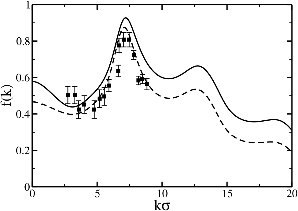
Figure 1: Non-ergodicity parameter. Lines: theoretical predictions at the ergodicity breaking transition; solid line: our theory, $\phi_{g}=.549$; dashed line: MCT, $\phi_{g}^{MCT}=.525$. Symbols: experimental data taken at $\phi=.563$ vanM .

The factorization approximation proposed here is the simplest possible one. There are two ways to improve upon it. First, one could try to include in an approximate way the off-diagonal blocks of $\mathcal{M}$. To this end one could express them in terms of a triple-density correlation function and then factorize this function into a product of three density correlation functions. Second, since the frequency matrix involves only static correlations, one could try to include it in a more sophisticated way. For example, one could include two-particle dynamics exactly Arun . The second extension could describe glassy dynamics in systems without static correlations SS .

To summarize, we proposed a new theory for dynamics of concentrated suspensions and the colloidal glass transition. The theory goes beyond MCT in that includes, in an approximate way, time-dependent pair-density fluctuations. In contrast to an earlier approachOppen , the present one uses pair-density correlation function evolving with one-particle irreducible dynamics. The new theory predicts an ergodicity breaking transition similar to that of MCT, but at a higher density.

The author benefited from inspiring discussions with Rolf Schilling and Arun Yethiraj; support by NSF Grant No. CHE-0111152 is gratefully acknowledged.

References

- (1) For a general introduction see, e.g., J.K.G. Dhont, An Introduction to Dynamics of Colloids (Elsevier, New York, 1996); for a very recent overview emphasizing connections between diffusional and viscoelastic properties see G. Nägele, J. Phys. Cond. Matter 15, S407 (2003).
- (2) See, e.g., W.K. Kegel and A. van Blaaderen, Science 287, 290 (2000); E.R. Weeks and D.A. Weitz, Phys. Rev. Lett. 89, 095704 (2002).
- (3) See, e.g., W. Härtl, Curr. Opin. Colloid Interface Sci. 6, 479 (2001), K.A. Dawson, ibid 7, 218 (2002).
- (4) M.E. Cates, cond-mat/0211066.
- (5) W. Götze, in Liquids, Freezing and Glass Transition, J.P. Hansen, D. Levesque, and J. Zinn-Justin, eds. (North-Holland, Amsterdam, 1991).
- (6) G. Szamel and H. Löwen, Phys. Rev. A 44, 8215 (1991).
- (7) This applies to systems in which hydrodynamic interactions can be neglected: strongly charged suspensions or simulated many-particle systems with Brownian dynamics. For real hard-sphere-like suspensions neglecting hydrodynamic interactions (or including them via a rescaling procedure (M. Medina-Noyola, Phys. Rev. Lett. 60, 2705 (1988))) constitutes an additional approximation; the importance of this approximation is largely unknown.
- (8) There are several ways to derive MCT. Here we discuss the original projection operator technique Goetze since it is the one used to derive the new theory.
- (9) Note that for Brownian systems one has to use irreducible memory function (S.J. Pitts and H.C. Andersen, J. Chem. Phys. 113, 3945 (2000); see also Ref. CHess ).
- (10) For Newtonian systems expressing the memory function in terms of pair-density correlation function neglects couplings to current modes. Within extended MCT currents restore ergodicity and cut off the ideal glass transition (W. Götze and L. Sjögren, Z. Phys. B 65, 415 (1987)).
- (11) G. Nägele and J. Bergenholtz, J. Chem. Phys. 108, 9893 (1998).
- (12) M. Fuchs and M.E. Cates, Phys. Rev. Lett. 89, 248304 (2002).
- (13) K.A. Dawson, G. Foffi, M. Fuchs, et al., Phys. Rev. E 63, 011401 (2001).
- (14) W. van Megen, S.M. Underwood, and P.N. Pusey, Phys. Rev. Lett. 67, 1586 (1991).
- (15) M. Nauroth and W. Kob, Phys. Rev. E 55, 657 (1997); this work discusses a Newtonian system; within MCT the location of the transition does not depend on the microscopic dynamics SL .
- (16) R. Schilling and G. Szamel, Europhys. Lett.61, 207 (2003).
- (17) C.Z.-W. Liu and I. Oppenheim, Physica A 247, 183 (1997).
- (18) For a similar idea in a different context see K. Miyazaki and A. Yethiraj, J. Chem. Phys. 117, 10448 (2002).
- (19) Following prior works on the colloidal glass transition, hydrodynamic interactions are neglected.
- (20) B. Cichocki and W. Hess, Physica A 141, 475 (1987).
- (21) Eq. (9) is exact for systems with pairwise-additive interactions.
- (22) G. Szamel, to be published.