Why social networks are different from other types of networks

Abstract

We argue that social networks differ from most other types of networks, including technological and biological networks, in two important ways. First, they have non-trivial clustering or network transitivity, and second, they show positive correlations, also called assortative mixing, between the degrees of adjacent vertices. Social networks are often divided into groups or communities, and it has recently been suggested that this division could account for the observed clustering. We demonstrate that group structure in networks can also account for degree correlations. We show using a simple model that we should expect assortative mixing in such networks whenever there is variation in the sizes of the groups and that the predicted level of assortative mixing compares well with that observed in real-world networks.

I Introduction

The last few years have seen a burst of interest within the statistical physics community in the properties of networked systems such as the Internet, the World Wide Web, and social and biological networks Strogatz01 ; AB02 ; DM03b ; Newman03d . Researchers’ attention has, to a large extent, been focused on properties that seem to be common to many different kinds of networks, such as the so-called “small-world effect” and skewed degree distributions WS98 ; BA99b ; ASBS00 . In this paper, by contrast, we highlight some apparent differences between networks, specifically between social and non-social networks. Our observations appear to indicate that social networks are fundamentally different from other types of networked systems.

We focus on two properties of networks that have received attention recently. First, we consider degree correlations in networks. It has been observed that the degrees of adjacent vertices in networks are positively correlated in social networks but negatively correlated in most other networks Newman02f . Second, we consider network transitivity or clustering, the propensity for vertex pairs to be connected if they share a mutual neighbor WS98 . We argue that the level of clustering seen in many non-social networks is no greater than one would expect by chance, given the observed degree distribution. For social networks however, clustering appears to be far greater than we expect by chance.

We conjecture that the explanation for both of these phenomena is in fact the same. Using a simple network model, we argue that if social networks are divided into groups or communities, this division alone can produce both degree correlations and clustering.

The outline of the paper is as follows. In Sec. II we discuss the phenomenon of degree correlation and summarize some empirical results for various networks. In Sec. III we do the same for clustering. We also present theoretical arguments that suggest that the clustering seen in non-social networks is of about the magnitude one would expect for a random graph model with parameters similar to real networks. Then in Sec. IV we present analytic results for a simple model of a social network divided into groups. This model, which was introduced previously Newman03e , is known to generate high levels of clustering. Here we show that it can also explain the presence of correlations between the degrees of adjacent vertices. In Sec. V we compare the model’s predictions concerning degree correlations against two real-world social networks, of collaborations between scientists and between businesspeople. In the former case we find that the model is in good agreement with empirical observation. In the latter we find that it can predict some but not all of the observed degree correlation, and we conjecture that the remainder is due to true sociological or psychological effects, as distinct from the purely topological effects contained in the model. In Sec. VI we give our conclusions.

II Degree correlations

In studies of the network structure of the Internet at the level of autonomous systems, Pastor-Satorras et al. PVV01 have recently demonstrated that the degrees of adjacent vertices in this network appear to be anticorrelated. They measured the mean degree $\langle k_{\rm nn}\rangle$ of the nearest neighbors of a vertex as a function of the degree $k$ of that vertex, and found that the resulting curve falls off with $k$ approximately as $\langle k_{\rm nn}\rangle\sim k^{-1/2}$. Thus, vertices of high degree $k$ tend to be connected, on average, to others of low degree, and vice versa. A simple way of quantifying this effect is to measure a correlation coefficient of the degrees of adjacent vertices in a network, defined as follows.

Suppose that $p_{k}$ is the degree distribution of our network, i.e., the fraction of vertices in the network with degree $k$, or equivalently the probability that a vertex chosen uniformly at random from the network will have degree $k$. The vertex at the end of a randomly chosen edge in the network will have degree distributed in proportion to $kp_{k}$, the extra factor of $k$ arising because $k$ times as many edges end at a vertex of degree $k$ than at a vertex of degree one Feld91 ; MR95 ; NSW01 . Commonly we are interested not in the total degree of the vertex at the end of an edge, but in the “excess degree,” which is the number of edges attached to the vertex other than the one we arrived along, which is obviously one less than the total degree. The properly normalized distribution of the excess degree is

$$q_{k}={(k+1)p_{k+1}\over\sum_{k}kp_{k}}.$$ (1)

We then define the quantity $e_{jk}$, which is the joint probability that a randomly chosen edge joins vertices with excess degrees $j$ and $k$.

Now consider a network in which the vertices have given degrees (the value of the degrees being called the “degree sequence”), but which is in all other respects random. That is, the network is drawn uniformly at random from the ensemble of all possible networks with the given degree sequence. This is the so-called configuration model Bollobas80 ; Luczak92 ; MR95 ; NSW01 , which we can use as a handy null model for testing our results. In the configuration model the expected value of the quantity $e_{jk}$ is simply $e_{jk}=q_{j}q_{k}$, and by its deviation from this value we can quantify the level of degree correlation present, relative to the null model. We define Newman02f

$$r={1\over\sigma_{q}^{2}}\sum_{jk}jk(e_{jk}-q_{j}q_{k}),$$ (2)

where $\sigma_{q}^{2}=\sum_{k}k^{2}q_{k}-\bigl{[}\sum_{k}kq_{k}\bigr{]}^{2}$ is the variance of the distribution $q_{k}$. The quantity $r$ will be positive or negative for networks with positive or negative degree correlations respectively. In the ecology and epidemiology literatures these two cases are called “assortative” and “disassortative” mixing by degree, and this nomenclature has been adopted by many physicists also.

The findings of Pastor-Satorras et al. PVV01 discussed above suggest that the Internet should have a negative value for $r$, and this indeed is the case. The most recent structural measurements of the autonomous-system graph of the Internet Chen02 yield a value of $r=-0.193\pm 0.002$. It now appears that similar results apply to essentially all other networks except social networks. In Refs. Newman02f and Newman03c we found that almost all networks seem to be disassortatively mixed, i.e., have negative values of the assortativity coefficient $r$, except for social networks, which are normally assortative. A small number of networks yield inconclusive results because the errors on $r$ are bigger than its value, but other than these few, the pattern appears essentially perfect.

Here we propose that this striking pattern arises because disassortativity is the natural state for all networks, in a sense that we will make clear shortly. Left to their own devices, we conjecture, networks normally have negative values of $r$. In order to show a positive value of $r$, a network must have some specific additional structure that favors assortative mixing. We suggest in Sec. IV that division into communities or groups provides such a structure in social networks.

Our conjecture that most networks will be disassortative is motivated by the work of Maslov et al. MSZ03 . Using computer simulations, they showed that on small networks, disassortative mixing is produced if one restricts the network topology to having at most one edge between any pair of vertices. The same result can be demonstrated analytically as well PN03 . How small a network need be to show this effect depends on the degree distribution; to see significant disassortativity, the highest-degree vertices in the network need to have degree on the order of $\sqrt{n}$, where $n$ is the total number of vertices, so that there is a substantial probability of some vertex pairs sharing two or more edges. (Obviously if there is negligible probability of a double edge occurring anywhere in the network, then the restriction of having no double edges will have no effect.) The Internet is a particularly good example of the effect, since it has a degree distribution that appears approximately to follow a power law, $p_{k}\sim k^{-\alpha}$ with $\alpha$ constant FFF99 ; Chen02 , and the fat tail of the power law produces many vertices of sufficiently high degree. However, a number of other networks also fit the bill: the World Wide Web, peer-to-peer networks, food webs, neural networks, and metabolic networks all have vertices of sufficiently high degree, at least in some cases. In their most common representations these networks also have only single edges between vertices, and hence we would expect them to have $r<0$, and calculations of $r$ from structural data confirm that this is the case Newman03c .

In fact, most networks have only single edges between their vertices. Although it is possible to have double edges in some networks, in practice these are usually ignored even where they exist and all edges are represented as single. For instance, in the World Wide Web it is possible, and even common, for a Web page to link twice or more to the same other page, creating a multiple link. Such links are however normally recorded as single by Web crawler programs, and hence any information about multiple links is lost. Thus many networks may have single edges only because that is the way researchers have chosen to represent them, and observed properties such as disassortativity may be purely a product of this choice of representation rather than a fundamental law of nature. Other networks may truly have single edges—metabolic networks and food-webs are possible examples of this.

Social networks also usually have only single edges between vertex pairs. Two people are either acquainted with one another or not—we do not normally have a concept of being “doubly acquainted” with a person. Nonetheless, the assortativity coefficient $r$ is positive, and sometimes very positive, for almost all social networks measured Newman02f ; Newman03c . This appears to indicate some special structure in social networks that distinguishes them from other types of networks. A revealing clue about what this special structure might be comes from network transitivity, as we now describe.

III Clustering

Watts and Strogatz WS98 have pointed out that most networks appear to have high transitivity, also called clustering. That is, the presence of a connection between vertices A and B, and another between B and C, makes it likely that there will also be a connection between A and C. To put it another way, if B has two network neighbors, A and C, they are likely to be connected to one another, by virtue of their common connection with B. In topological terms, there is a high density of triangles, ABC, in the network, and clustering can be quantified by measuring this density:

$$C={\mbox{$3\times$ number of triangles on the graph}\over\mbox{number of connected triples of vertices}},$$ (3)

where a “connected triple” means a vertex connected directly to an unordered pair of others. In physical terms, $C$ is the probability, averaged over the network, that two of your friends will be friends also of one another. (This is in fact only one definition of the clustering coefficient. An alternative definition, given in WS98 , has also been widely used. The latter however is difficult to evaluate analytically, and so we avoid it here.)

The value of the clustering coefficient in the null configuration model can be calculated in a straightforward fashion Newman03b ; EMB02 . Suppose that two neighbors of the same vertex have excess degrees $j$ and $k$. The probability that one particular edge in the network falls between these two vertices is $2\times j/(2m)\times k/(2m)$, where $m$ is the total number of edges in the network. The total number of edges between the two vertices in question is $m$ times this quantity, or $jk/(2m)$. Both $j$ and $k$ are distributed according to (1), since both vertices are neighbors of A and, averaging over this distribution, we then get an expression for the clustering coefficient:

$$C={1\over 2m}\,\Bigl{[}\sum_{k}kq_{k}\Bigr{]}^{2}={1\over n}\,{\bigl{[}\langle k^{2}\rangle-\langle k\rangle\bigr{]}^{2}\over\langle k\rangle^{3}},$$ (4)

where averages are over all vertices and we have made use of $2m=n\langle k\rangle$.

Normally this quantity goes as $n^{-1}$ and so is very small for large graphs. However, some graphs are not large, and hence $C$ is not negligible. Consider for example the foodweb of organism in Little Rock Lake, WI, which was originally analyzed by Martinez Martinez91 and has been widely studied in the networks literature. This network has $n=92$, $\langle k\rangle=21.0$, and $\langle k^{2}\rangle=655.2$. Plugging these figures into Eq. (4) gives $C=0.47$. The measured value of $C$ is $0.40$. Thus it appears that we need invoke no special clustering process to explain the clustering in this network. Similar results can be found for other small networks.

This argument can also be applied to some larger networks as well, particularly those with power-law degree distributions. The fat tail of the degree distribution in power-law networks can affect the value of the clustering coefficient strongly. To see this consider first how the degree of the highest-degree vertex in the configuration model varies with system size Newman03d .

The probability of there being exactly $m$ vertices of degree $k$ in the network and no vertices of degree greater than $k$ is ${n\choose m}p_{k}^{m}(1-P_{k})^{n-m}$, where

$$P_{k}=\sum_{k^{\prime}=k}^{\infty}p_{k^{\prime}},$$ (5)

is the probability that a vertex has degree greater than or equal to $k$. Then the probability $h_{k}$ that the highest degree in the network is $k$ is

$$h_{k} = \sum_{m=1}^{n}{n\choose m}p_{k}^{m}(1-P_{k})^{n-m}$$ (6)

$$= (p_{k}+1-P_{k})^{n}-(1-P_{k})^{n},$$

and the expected value of the highest degree is $k_{\mathrm{max}}=\sum_{k}kh_{k}$.

The value of $h_{k}$ tends to zero for both small and large values of $k$, and the sum over $k$ is dominated by the terms close to the maximum. Thus, in most cases, a good approximation to the expected value of the maximum degree is given by the modal value. Differentiating and observing that ${\rm d}P_{k}/{\rm d}k=p_{k}$, we find that the maximum of $h_{k}$ occurs when

$$\biggl{(}{{\rm d}p_{k}\over{\rm d}k}-p_{k}\biggr{)}(p_{k}+1-P_{k})^{n-1}+p_{k}(1-P_{k})^{n-1}=0,$$ (7)

or $k_{\mathrm{max}}$ is a solution of

$${{\rm d}p_{k}\over{\rm d}k}\simeq-np_{k}^{2},$$ (8)

where we have made the assumption that $p_{k}$ is sufficiently small for $k\gtrsim k_{\mathrm{max}}$ that $np_{k}\ll 1$ and $P_{k}\ll 1$. For a degree distribution with a power-law tail $p_{k}\sim k^{-\alpha}$, we then find that

$$k_{\mathrm{max}}\sim n^{1/(\alpha-1)}.$$ (9)

(As shown by Cohen et al. CEBH00 , a simple rule of thumb that leads to the same result is that the maximum degree is roughly the value of $k$ that solves $nP_{k}=1$.)

Most networks of interest have $\alpha<3$, which means $\langle k^{2}\rangle\sim k_{\mathrm{max}}^{3-\alpha}\sim n^{(3-\alpha)/(\alpha-1)}$ and $\langle k\rangle$ is independent of $n$. Then (4) gives

$$C\sim n^{(7-3\alpha)/(\alpha-1)}.$$ (10)

If $\alpha>\frac{7}{3}$, this means that $C$ tends to zero as the graph becomes large, although it does so slower than the explicit $C\sim n^{-1}$ of Eq. (4). At $\alpha=\frac{7}{3}$, $C$ becomes constant (or logarithmic) in the graph size. And remarkably, for $\alpha<\frac{7}{3}$ it actually increases with increasing system size, becoming arbitrarily large as $n\to\infty$. Thus for $\alpha\lesssim\frac{7}{3}$, we might expect to see quite large values of $C$ even in large networks.

Taking the case of the World Wide Web, for example, we find the predicted value of the clustering coefficient for the configuration model is $C=0.048$ Newman03b , while the measured value is $0.11$—certainly not perfect agreement, but of the right order of magnitude. Other examples err in the opposite direction. Maslov et al. MSZ03 for instance cite the example of the Internet, for which they show using numerical simulations that the observed clustering is actually lower than that expected for an equivalent random graph model.

It is worth noting that Eq. (10) implies the clustering coefficient can be greater than 1 if $\alpha<\frac{7}{3}$. Physically this means that there will be more than one edge on average between two vertices that share a common neighbor. This is perhaps at odds with the conventional interpretation of the clustering coefficient as the probability that there exists any edge between the given two vertices—normally one would not distinguish between the case where there are two edges and the case where there is one. (Indeed, as mentioned in Sec. II, in many networks, one ignores double edges altogether.) If one takes this approach, then the value of the clustering coefficient is modified for networks that would otherwise have $C>1$ as follows.

Consider again two vertices that are neighbors of vertex A, with excess degrees $j$ and $k$. The probability that a particular edge falls between them is $2\times j/(2m)\times k/(2m)$, as before, and the probability that it does not is 1 minus this quantity. Then the probability that no edge falls between this pair is

$$\biggl{[}1-{jk\over 2m^{2}}\biggr{]}^{m}\simeq{\rm e}^{-jk/2m},$$ (11)

where the equality becomes exact in the limit of large $m$. Thus the probability of any edge falling between the two vertices is $1-{\rm e}^{-jk/2m}$, and the correct expression for the clustering coefficient is the average of this:

$$C=\sum_{jk}q_{j}q_{k}\bigl{(}1-{\rm e}^{-jk/2m}\bigr{)}.$$ (12)

In fact, however, using this expression makes only the smallest of differences to the expected value of $C$ on, for example, the World Wide Web.

All of this demonstrates that for many non-social networks, including foodwebs, the Internet, and the World Wide Web, clustering can be explained by a simple random model. The same however is not true of social networks. It turns out that social networks in general have a far higher degree of clustering than the corresponding random model. We give four examples: the widely studied network of film-actor collaborations WS98 ; ASBS00 , collaboration networks of mathematicians GI95 ; BM00 and company directors DYB01 , and an email network NFB02 . For these four networks the theory presented above predicts values of the clustering coefficient of $0.0098$, $0.00015$, $0.0035$, and $0.017$. The actual measured values are $0.20$, $0.15$, $0.59$, and $0.17$, in each case at least an order of magnitude greater than the prediction. The implication appears to be that there is some mechanism producing clustering in social networks that is not present at a significant level in non-social networks (or not at least in the examples studied here). Recent work GN02 ; Guimera03 ; RB03 ; Newman03e ; TWH03 suggests a possible candidate theory, that social networks contain groups, or “community structure” .

IV Community structure in networks

In Newman03e one of us proposed a simple model of a network with community structure and showed that this structure produces substantial clustering, with values of $C$ that do not go to zero as the network size becomes large. Thus the results of the preceding section could be explained if social networks possess community structure and other types of networks do not (or they possess it to a lesser degree). We now show that the same distinction can also explain the observed difference in degree correlations between social and non-social networks.

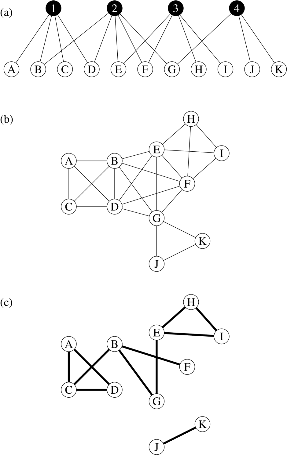
Figure 1: The structure of the network model studied in Sec. IV. (a) We represent individuals (A–K) and the groups (1–4) to which they belong with a bipartite graph structure. (b) The bipartite graph is projected onto the individuals only, giving a network with edges between any pair of individuals who share a group. (c) The actual social connections between individuals are chosen by bond percolation on this projection with bond occupation probability $p$. The net result is that individuals have probability $p$ of knowing others with whom they share a group.

In our model the network is divided into groups and each individual can belong to any number of groups. Individuals do not necessarily know all those with whom they share a group, but instead have probability $p$ of acquaintance. They have probability zero of knowing those with whom they do not share a group. Mathematically the model can be represented as a bond percolation process with occupation probability $p$ on the network formed by the projection of a suitable bipartite graph of individuals and groups onto just the individuals, as shown in Fig. 1. The percolation properties of the model can be solved exactly using generating function methods.

In Newman03e the model was studied in a simple version in which the size of all groups was assumed the same. This case can account for the presence of clustering in the network, and is straightforward to treat mathematically. However, it is inadequate for our purposes here, since it does not produce any degree correlation. Degree correlation arises because individuals who belong to small groups tend to have low degree and are connected to others in the same group, who also have low degree. Similarly those in large groups tend to have higher degree and are also connected to one another. Thus, the model should give rise to assortative mixing provided there is enough variation in the sizes of groups. As we will see, this is indeed the case.

In addition to the parameter $p$, we characterize the model by two probability distributions: $r_{m}$ is the probability that an individual belongs to $m$ groups and $s_{n}$ is the probability that a group contains $n$ individuals. Subject to the constraints imposed by these distributions, the assignment of individuals to groups is entirely random.

To proceed we calculate the joint distribution $e_{jk}$ of the excess degrees of vertices at the ends of an edge. Noting that the total number of edges in groups of size $n$ goes as $s_{n}n(n-1)$, we write

$$e_{jk}=e_{0}\sum_{n}s_{n}n(n-1)P(j,k|n)$$ (13)

where $P(j,k|n)$ is the probability that an edge that belongs to a group of size $n$ connects vertices of excess degrees $j$ and $k$, and $e_{0}$ is a constant whose value can be calculated from the requirement that $e_{jk}$ be normalized, so that $\sum_{jk}e_{jk}=1$.

We now decompose $j$ and $k$ in the form $j=j_{\mathrm{in}}+j_{\mathrm{out}}$, $k=k_{\mathrm{in}}+k_{\mathrm{out}}$, where $j_{\mathrm{in}}$, $k_{\mathrm{in}}$ are the numbers of connections to vertices within the group that the two vertices share, and $j_{\mathrm{out}}$, $k_{\mathrm{out}}$ are the numbers of connections outside that group. The distributions of $j_{\mathrm{in}}$ and $k_{\mathrm{in}}$ are simply binomial, and hence $P(j,k|n)$ factors into terms depending only on $j$ and $k$ thus:

$$P(j,k|n) = \sum_{j_{\mathrm{in}}}{n-2\choose j_{\mathrm{in}}}p^{j_{\mathrm{in}}}q^{n-2-j_{\mathrm{in}}}P(j_{\mathrm{out}})$$ (14)

$${}\times\sum_{k_{\mathrm{in}}}{n-2\choose k_{\mathrm{in}}}p^{k_{\mathrm{in}}}q^{n-2-k_{\mathrm{in}}}P(k_{\mathrm{out}}),$$

where $P(j_{\mathrm{out}})$ is the probability distribution of $j_{\mathrm{out}}$, which is independent of $j_{\mathrm{in}}$, and similarly for $k_{\mathrm{out}}$.

To evaluate this expression we introduce the following generating functions for the distributions $r_{m}$ and $s_{n}$:

$$f_{0}(z) = \!\sum_{m=0}^{\infty}r_{m}z^{m},\hskip 8.0ptf_{1}(z)={1\over f_{0}^{\prime}(1)}\sum_{m=0}^{\infty}mr_{m}z^{m-1},$$ (15)

$$g_{0}(z) = \sum_{n=0}^{\infty}s_{n}z^{n},\hskip 12.2ptg_{1}(z)={1\over g_{0}^{\prime}(1)}\sum_{n=0}^{\infty}ns_{n}z^{n-1}.$$ (16)

Physically, $f_{0}(z)$ is the generating function for the number of groups an individual belongs to, and $f_{1}(z)$ is the generating function for the number groups that an individual in a randomly selected group belongs to, other than the randomly selected group itself. Similarly $g_{0}(z)$ generates the group sizes and $g_{1}(z)$ generates the number of other individuals in a group to which a randomly selected individual belongs. Of these others, our randomly selected individual is connected to a number binomially distributed according to the probability $p$ and thus generated by the simple generating function $pz+q$, where $q=1-p$. Averaging over the group sizes, the number of neighbors of a randomly chosen individual within one of the groups to which they belong is generated by $g_{1}(pz+q)$, and an individual belonging to a randomly chosen group will have a number of neighbors in other groups generated by $f_{1}(g_{1}(pz+q))$. This then gives us precisely the quantity $P(j_{\mathrm{out}})$ of Eq. (14), which is equal to the coefficient of $z^{j_{\mathrm{out}}}$ in $f_{1}(g_{1}(pz+q))$, and similarly for $P(k_{\mathrm{out}})$.

Combining Eqs. (13) and (14) we find that $e_{jk}$ is generated by the double probability generating function

$$E(x,y) = \sum_{jk}e_{jk}x^{j}y^{k}$$ (17)

$$= g_{2}\bigl{(}(px+q)(py+q)\bigr{)}$$

$$\quad{}\times f_{1}(g_{1}(px+q))f_{1}(g_{1}(py+q)),$$

where

$$g_{2}(z)=\frac{1}{g_{0}^{\prime\prime}(1)}\sum_{n=0}^{\infty}n(n-1)s_{n}z^{n-2}.$$ (18)

Then, making use of Eqs. (1) and (2) and the fact that $q_{k}=\sum_{j}e_{jk}$, we can write the assortativity coefficient $r$ as

$$r=\frac{\partial_{x}\partial_{y}E-(\partial_{x}E)\,(\partial_{y}E)}{\partial_{x}(x\,\partial_{x}E)-(\partial_{x}E)\,(\partial_{y}E)}\Biggr{|}_{x=y=1}={\mathcal{P}\over\mathcal{Q}},$$ (19)

where the numerator and denominator $\mathcal{P}$ and $\mathcal{Q}$ are

$$\mathcal{P} = p\mu_{1}^{2}\nu_{1}^{2}\bigl{[}(\nu_{4}-\nu_{3})(\nu_{2}-\nu_{1})-(\nu_{3}-\nu_{2})^{2}\bigr{]}$$ (20a)

$$\mathcal{Q} = \mu_{1}\nu_{1}(\nu_{2}-\nu_{1})\bigl{[}(\mu_{2}-\mu_{1})(\nu_{2}-\nu_{1})^{2}+\mu_{1}\nu_{1}(2\nu_{1}-3\nu_{2}+\nu_{3})\bigr{]}$$ (20b)

$$\quad{}+p\bigl{[}(\mu_{1}^{2}-\mu_{2}^{2}-\mu_{1}\mu_{2}+\mu_{1}\mu_{3})(\nu_{2}-\nu_{1})^{4}+\mu_{1}\mu_{2}\nu_{1}(\nu_{2}-\nu_{1})^{2}(2\nu_{1}-3\nu_{2}+\nu_{3})$$

$$\quad{}+\mu_{1}^{2}\nu_{1}\bigl{(}\nu_{1}^{2}(2\nu_{2}+\nu_{3}-\nu_{4})-\nu_{1}(\nu_{3}-\nu_{2})^{2}-\nu_{1}\nu_{2}(\nu_{4}-5\nu_{2})+\nu_{2}^{2}(3\nu_{2}-\nu_{3})\bigr{)}\bigr{]}$$

In this expression the quantities $\mu_{n}$ and $\nu_{n}$ are the $n$th moments of the distributions $r_{m}$ and $s_{n}$ respectively. Thus, given the distributions and the probability $p$ it is elementary, if tedious, to calculate $r$. Below we apply this expression to two real-world example networks. First, however, a few points are worth noting.

It is straightforward to show, though certainly not obvious to the eye, that the expression for $r$, Eq. (19), is non-negative for all distributions $r_{m}$ and $s_{n}$, so that our model always produces an assortatively mixed network, as our intuition suggests.

Now consider the simple case in which each individual belongs to exactly one group, and the group sizes have a Poisson distribution. In this case, Eq. (19) gives $r=p$, and we can achieve any value of $r$ by tuning the parameter $p$. In particular, if each individual knows all others in their group then $p=1$ and we have perfect assortativity. This is reasonable, since in this case each individual in a group has the exact same number of neighbors. This case is a rather pathological one however, since if everyone belongs to only one group, then the network consists of many isolated groups and most people are not connected to one another. To make things more realistic, let us allow the number of groups to which individuals belong also to vary according to a Poisson distribution. Then we find that

$$r=\frac{p}{1+\mu+\nu\mu p},$$ (21)

where $\mu\equiv\mu_{1}$ and $\nu\equiv\nu_{1}$ are the means of the two distributions. Thus as the two means increase, the correlation decreases. The decrease with $\mu$ is easily understood—the more groups an individual belongs to, the less the relative within-group degree correlation upon which the assortativity depends: the within-group correlation is diluted by all the other groups the individual belongs to. The behavior with $\nu$ is a little more subtle. The width of the Poisson distribution of group sizes goes as $1/\sqrt{\nu}$ as a fraction of the mean, and hence the effective variation in size between groups decreases with increasing $\nu$. It is this decrease that drives $r$ towards zero.

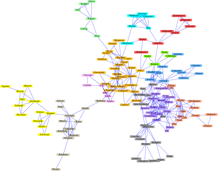
Figure 2: The largest component of the network of coauthorships described in the text. This component contains 142 scientists, and there are 36 other components, of sizes ranging from 1 to 5, containing 84 more. The vertices are colored according to the communities found using the algorithm of Ref. GN02 . The communities correspond reasonably closely to geographical and institutional divisions between the scientists shown.

V Examples

We now apply our model to two real-world example networks. In the first case, as we will see, it gives a value of $r$ in excellent agreement with the real network. In the second it underestimates $r$ by about a factor of two, indicating that group structure can account for only a portion of the observed assortativity, the rest, we conjecture, being due to true social effects.

V.1 Collaboration network

Networks of coauthorship of scientists or other academics provide some of the best-documented examples of social networks GI95 ; Newman01a . Using bibliographic databases it is possible to construct large coauthorship networks with high reliability, and these networks are true social networks, in the sense that it seems highly likely that two authors who write a paper together are acquainted.

Fig. 2 shows a coauthorship network of physicists who conduct research on networks. The network was constructed using names drawn from the large bibliography of Ref. Newman03d and coauthorship data from preprints submitted to the condensed matter section of the Physics E-print Archive at arxiv.org between Jan 1, 1995 and April 30, 2003. To find the groups in the network, we fed it through the community structure algorithm of Girvan and Newman GN02 , producing the division shown by the colors in the figure. The figure shows only the largest component of the network. There are also 36 smaller components, which were included in our calculations even though they are not shown.

The moments of the distributions $r_{m}$ and $s_{n}$ are easily extracted from the network by direct summation. To find the value of $p$, we counted the number of edges in the network and divided by the total number of possible within-group edges, giving $p=0.178$. Feeding this value and our figures for the moments into Eqs. (19) and (20), we then find a predicted value of $r=0.145$. The measured value for the real network is $0.174\pm 0.045$. (The error is calculated according to the prescription given in Newman03c .) These two figures are in agreement within the statistical error on the latter.

While this result by no means proves that the group structure is responsible for assortativity in this network, it tells us that no other assumption is necessary to give the observed value of $r$. With group structure as shown in the figure and otherwise random mixing, we would get a network with exactly the assortativity that is observed in reality, within expected error.

V.2 Boards of directors

Davis and collaborators DG97 ; DYB01 have studied networks of the directors of companies in which two directors are considered connected if they sit on the board of the same company. They studied the Fortune 1000, the one thousand US companies with the highest revenues, for 1999, and assembled a near-complete director network from publicly available data. The network consists of 7673 directors sitting on 914 boards. It provides a particularly simple example of our method, for two reasons. First, the groups in the network through which individuals are acquainted are provided for us—they are the boards of directors. Second, it is assumed that directors are acquainted with all those with whom they share a board, so that the parameter $p$ in our model is 1.

The distributions of boards per director and directors per board have been studied before NSW01 . We note that most directors (79%) sit on only one board and that there is considerable variation in the size of boards (from 2 to 35 members). Thus we would expect strong assortative mixing in the network, and indeed we find that $r=0.276\pm 0.004$. Taking the moments of the measured distributions $r_{m}$ and $s_{n}$ for the network and setting $p=1$, Eq. (19) gives a value of $r=0.116$ for our model. So it appears that the presence of groups in the network can explain about 40% of the assortativity we observe in this case, but not all of it. There is some additional assortativity in addition to the purely topological effect of the groups, and we conjecture that this is due to some true sociological or psychological effect in the way in which acquaintanceships are formed. One possibility is suggested by the analysis of the directorships data by Newman et al. NSW01 , who found that directors who sit on many boards tend to sit on them with others who sit on many boards. Since those who sit on many boards will also tend to have high degree, we would expect this effect to add assortativity to the network, but the effect is missing from our model in which board membership is assigned at random.

In a sense, our model is giving a baseline against which to measure the value of $r$; it tells us when the value we see is simply what would be expect by random chance, as in the collaboration network above, and when there must be additional effects at work, as in the boards of directors.

VI Conclusions

In this paper we have argued that social and non-social networks differ in two important ways. First, they show distinctly different patterns of correlation between the degrees of adjacent vertices, with degrees being positively correlated (assortative mixing) in most social networks and negatively correlated (disassortative mixing) in most non-social networks. Second, social networks show high levels of clustering or network transitivity, whereas clustering in many non-social networks is no higher than one would expect on the basis of pure chance, given the observed degree distribution.

We have shown that both of these differences can be explained by the same hypothesis, that social networks are divided into communities, and non-social networks are not. We have studied a simple model of community structure in social networks in which individuals belong to groups and are acquainted with others with whom they share those groups. The model is exactly solvable using generating function techniques, and we have shown that it gives predictions that are in reasonable and sometimes excellent agreement with empirical observations of real-world social networks.

- (1) S. H. Strogatz, Exploring complex networks. Nature 410, 268–276 (2001).
- (2) R. Albert and A.-L. Barabási, Statistical mechanics of complex networks. Rev. Mod. Phys. 74, 47–97 (2002).
- (3) S. N. Dorogovtsev and J. F. F. Mendes, Evolution of Networks: From Biological Nets to the Internet and WWW. Oxford University Press, Oxford (2003).
- (4) M. E. J. Newman, The structure and function of complex networks. SIAM Review 45, 167–256 (2003).
- (5) D. J. Watts and S. H. Strogatz, Collective dynamics of ‘small-world’ networks. Nature 393, 440–442 (1998).
- (6) A.-L. Barabási and R. Albert, Emergence of scaling in random networks. Science 286, 509–512 (1999).
- (7) L. A. N. Amaral, A. Scala, M. Barthélémy, and H. E. Stanley, Classes of small-world networks. Proc. Natl. Acad. Sci. USA 97, 11149–11152 (2000).
- (8) M. E. J. Newman, Assortative mixing in networks. Phys. Rev. Lett. 89, 208701 (2002).
- (9) M. E. J. Newman, Properties of highly clustered networks. Preprint cond-mat/0303183 (2003).
- (10) R. Pastor-Satorras, A. Vázquez, and A. Vespignani, Dynamical and correlation properties of the Internet. Phys. Rev. Lett. 87, 258701 (2001).
- (11) S. Feld, Why your friends have more friends than you do. Am. J. Sociol. 96, 1464–1477 (1991).
- (12) M. Molloy and B. Reed, A critical point for random graphs with a given degree sequence. Random Structures and Algorithms 6, 161–179 (1995).
- (13) M. E. J. Newman, S. H. Strogatz, and D. J. Watts, Random graphs with arbitrary degree distributions and their applications. Phys. Rev. E 64, 026118 (2001).
- (14) B. Bollobás, A probabilistic proof of an asymptotic formula for the number of labelled regular graphs. European Journal on Combinatorics 1, 311–316 (1980).
- (15) T. Łuczak, Sparse random graphs with a given degree sequence. In A. M. Frieze and T. Łuczak (eds.), Proceedings of the Symposium on Random Graphs, Poznań 1989, pp. 165–182, John Wiley, New York (1992).
- (16) Q. Chen, H. Chang, R. Govindan, S. Jamin, S. J. Shenker, and W. Willinger, The origin of power laws in Internet topologies revisited. In Proceedings of the 21st Annual Joint Conference of the IEEE Computer and Communications Societies, IEEE Computer Society (2002).
- (17) M. E. J. Newman, Mixing patterns in networks. Phys. Rev. E 67, 026126 (2003).
- (18) S. Maslov, K. Sneppen, and A. Zaliznyak, Pattern detection in complex networks: Correlation profile of the Internet. Preprint cond-mat/0205379 (2002).
- (19) J. Park and M. E. J. Newman, The origin of degree correlations in the Internet and other networks. Preprint cond-mat/0303327 (2003).
- (20) M. Faloutsos, P. Faloutsos, and C. Faloutsos, On power-law relationships of the internet topology. Computer Communications Review 29, 251–262 (1999).
- (21) M. E. J. Newman, Random graphs as models of networks. In S. Bornholdt and H. G. Schuster (eds.), Handbook of Graphs and Networks, pp. 35–68, Wiley-VCH, Berlin (2003).
- (22) H. Ebel, L.-I. Mielsch, and S. Bornholdt, Scale-free topology of e-mail networks. Phys. Rev. E 66, 035103 (2002).
- (23) N. D. Martinez, Artifacts or attributes? Effects of resolution on the Little Rock Lake food web. Ecological Monographs 61, 367–392 (1991).
- (24) R. Cohen, K. Erez, D. ben-Avraham, and S. Havlin, Resilience of the Internet to random breakdowns. Phys. Rev. Lett. 85, 4626–4628 (2000).
- (25) J. W. Grossman and P. D. F. Ion, On a portion of the well-known collaboration graph. Congressus Numerantium 108, 129–131 (1995).
- (26) V. Batagelj and A. Mrvar, Some analyses of Erdős collaboration graph. Social Networks 22, 173–186 (2000).
- (27) G. F. Davis, M. Yoo, and W. E. Baker, The small world of the corporate elite. Preprint, University of Michigan Business School (2001).
- (28) M. E. J. Newman, S. Forrest, and J. Balthrop, Email networks and the spread of computer viruses. Phys. Rev. E 66, 035101 (2002).
- (29) M. Girvan and M. E. J. Newman, Community structure in social and biological networks. Proc. Natl. Acad. Sci. USA 99, 8271–8276 (2002).
- (30) R. Guimerà, L. Danon, A. Díaz-Guilera, F. Giralt, and A. Arenas, Self-similar community structure in organisations. Preprint cond-mat/0211498 (2002).
- (31) E. Ravasz and A.-L. Barabási, Hierarchical organization in complex networks. Phys. Rev. E 67, 026112 (2003).
- (32) J. R. Tyler, D. M. Wilkinson, and B. A. Huberman, Email as spectroscopy: Automated discovery of community structure within organizations. Preprint cond-mat/0303264 (2003).
- (33) M. E. J. Newman, The structure of scientific collaboration networks. Proc. Natl. Acad. Sci. USA 98, 404–409 (2001).
- (34) G. F. Davis and H. R. Greve, Corporate elite networks and governance changes in the 1980s. Am. J. Sociol. 103, 1–37 (1997).
- (35) D. L. Banks and K. M. Carley, Models for network evolution. Journal of Mathematical Sociology 21, 173–196 (1996).
- (36) D. J. Watts, Networks, dynamics, and the small world phenomenon. Am. J. Sociol. 105, 493–592 (1999).
- (37) E. M. Jin, M. Girvan, and M. E. J. Newman, The structure of growing social networks. Phys. Rev. E 64, 046132 (2001).
- (38) J. Davidsen, H. Ebel, and S. Bornholdt, Emergence of a small world from local interactions: Modeling acquaintance networks. Phys. Rev. Lett. 88, 128701 (2002).
- (39) K. Klemm and V. M. Eguiluz, Highly clustered scale-free networks. Phys. Rev. E 65, 036123 (2002).
- (40) J. Jost and M. P. Joy, Evolving networks with distance preferences. Phys. Rev. E 66, 036126 (2002).