High Tc Superconductors: A Variational Theory of the Superconducting State

Abstract

We use a variational approach to gain insight into the strongly correlated d-wave superconducting state of the high Tc cuprates at T=0. We show that strong correlations lead to qualitatively different trends in pairing and phase coherence: the pairing scale decreases monotonically with hole doping while the SC order parameter shows a non-monotonic dome. We obtain detailed results for the doping-dependence of a large number of experimentally observable quantities, including the chemical potential, coherence length, momentum distribution, nodal quasiparticle weight and dispersion, incoherent features in photoemission spectra, optical spectral weight and superfluid density. Most of our results are in remarkable quantitative agreement with existing data and some of our predictions, first reported in Phys. Rev. Lett. 87, 217002 (2001), have been recently verified.

I Introduction

In this paper our main goal is to understand the superconducting ground state and low energy excitations of the high Tc cuprates, in particular, their doping dependence as they evolve from a Fermi liquid state on the overdoped side towards a Mott insulator at half-filling. Toward this end, we examine in detail the properties of superconducting wavefunctions in which double occupancy is strongly suppressed by short-range Coulomb interactions.

In the past seventeen years since the discovery of high Tc superconductivity (SC) in the cuprates hightc86 , a lot of theoretical effort has gone into trying to understand SC as an instability from a non-superconducting state. There are three possible routes to such an attack and each has its own strengths and limitations. First, one may approach the SC state from the overdoped side, where the normal state is a well-understood Fermi liquid. However, the diagrammatic methods used in such an approach are not adequate for addressing the most interesting underdoped region in the vicinity of the Mott insulator. Second, one might hope to examine the SC instability from the near-optimal normal state, except that this normal state is highly abnormal and the breakdown of Fermi-liquid behavior remains one of the biggest open questions in the field. The third approach is to enter the SC state as a doping-driven instability from the Mott insulator. While this approach has seen considerable theoretical progress, much of the discussion is complicated by various broken symmetries and competing instabilities in lightly doped Mott insulators.

Here we take a rather different approach, in which we do not view superconductivity as an instability from any non-SC state, but rather study the SC state in and of itself. After all, the main reason for interest in the cuprates comes from their superconductivity, and not from other possible orders, which may well exist in specific materials in limited doping regimes. Thus it is very important to theoretically understand the SC state in all its details, particularly capturing both the BCS-like behavior on the overdoped side and the non-BCS aspects, like the large spectral gap but low Tc and superfluid density, on the underdoped side. The resulting insights could also help in characterizing the anomalous normal states which are obtained upon destroying the SC order.

We choose to work within a two-dimensional, single-band approach with strong local electron-electron interactions, described by the large $U$ Hubbard model, first advocated by Anderson anderson87 for the cuprate superconductors. Our goal is to see how much of the physics of the cuprates can be captured within this framework. To the extent that this approach proves inadequate, one may need to go beyond it and include either long-range Coulomb interactions, additional bands, inter-layer effects, or even phonons. The success of our approach reported here suggest to us that, at least for the SC state properties studied, one does not need to explicitly include these additional degrees of freedom.

The key technical challenge is to treat the effect of strong correlations in a controlled manner. We have chosen to deal with this using Gutzwiller wavefunctions and using the variational Monte Carlo method to evaluate various expectation values building on pioneering work by several authors anderson87 ; fczhang ; gros88 ; shiba88 .

We now summarize our main results; this also serves as an outline of the remainder of the paper. Some of these results were first reported in a Letter paramekanti01 .

$\bullet$ We introduce in Sec. IV our wavefunction which is a fully projected d-wave BCS state, in which all configurations with doubly occupied sites are first eliminated, and the effects of the finite Coulomb $U$ are then built in via a canonical transformation described in Sec. III.

$\bullet$ Using a variational calculation, we obtain in Sec. V.B the following $T=0$ phase diagram: a Fermi liquid metal for hole concentrations $x>x_{c}\approx 0.35$, a strongly correlated d-wave SC for $0<x<x_{c}$, and a spin-liquid Mott insulator at $x=0$.

$\bullet$ The pairing, as characterized by our variational parameter $\Delta_{\rm var}(x)$, is a monotonically decreasing function of hole doping $x$, largest at $x=0$ and vanishing beyond $x_{c}$; see Fig. 1(a). In marked contrast, the SC order parameter $\Phi(x)$ shows a nonmonotonic doping dependence; see Fig. 3(a).

$\bullet$ The nonmonotonic SC order parameter naturally gives rise to the notion of optimal doping $x\simeq 0.2$ at which superconductivity is the strongest. We explain in detail in Sec. V.B this nonmonotonic behavior and, in particular, how strong correlations – and not a competing order – lead to a suppression of superconductivity as $x\to 0$ despite the presence of strong pairing.

$\bullet$ We predict a nonmonotonic doping dependence for the SC coherence length, $\xi_{\rm sc}$, which diverges both as $x\to 0^{+}$ and as $x\to x_{c}^{-}$, but is small, of order few lattice spacings at optimal doping; see Fig. 3(b) and Sec. V.C.

$\bullet$ We study the momentum distribution $n({\bf k})$ and its doping dependence in Sec. VI, and find that the “Fermi surface” derived from $n({\bf k})$ is consistent with angle-resolved photoemission spectroscopy (ARPES) experiments and very similar to the non-interacting band-theory result.

$\bullet$ Using the singularities of the moments of the electronic spectral function, we characterize in detail the low-lying excitations of the SC state in Secs. VII and VIII. We obtain, for the first time, the doping dependence of the coherent weight $Z$ and Fermi velocity $v_{{}_{F}}$ of nodal quasiparticles (QP) and make predictions for the nodal QP self-energy. Remarkably, $Z$ vanishes as $x\to 0$, however $v_{{}_{F}}$ is essentially doping independent and finite as $x\to 0$. Our predictions paramekanti01 for the magnitudes and doping dependence of the nodal $Z$ and $v_{{}_{F}}$ have been verified by new ARPES experiments as discussed in Sec. VIII.

$\bullet$ We demonstrate, using moments of the electronic spectral function, that strong correlations lead to large incoherent spectral weight which is distributed over a large energy scale. Specifically, we relate our variational parameter $\Delta_{\rm var}(x)$ to an incoherent energy scale at ${\bf k}=(\pi,0)$ in Sec. IX. This motivates us to compare $\Delta_{\rm var}$ with the incoherent $(\pi,0)$ “hump” scale in ARPES. As seen from Fig. 8, once we scale $\Delta_{\rm var}$ to agree with the data at one doping value, we find excellent agreement between the two for all doping levels.

$\bullet$ We compute in Sec. X the total optical spectral weight $D_{\rm tot}$ and the low frequency optical spectral weight or Drude weight $D_{\rm low}$; see Fig. 10(a). The Drude weight, which vanishes with underdoping, is in good quantitative agreement with optics experiments.

$\bullet$ We predict that the Drude weight $D_{\rm low}\sim Z$ nodal QP weight, in the entire SC regime, which could be tested by comparing optics and ARPES experiments.

$\bullet$ We use the calculation of $D_{\rm low}$ to obtain an upper bound on the superfluid density, leading to the conclusion that the superfluid density vanishes as $x\to 0$, consistent with experiments. The underdoped regime thus has strong pairing but very small phase stiffness leading to a pairing pseudogap above $T_{c}$.

This is first time that such a wealth of information has been obtained on correlated SC wavefunctions which permits useful comparison with and predictions for a variety of experiments. Further, as we will emphasize later in the text, many qualitative features of our results in the underdoped region, such as the incoherence in the spectral function and the doping dependence of quantities like the SC order parameter, nodal QP weight, and Drude weight are mainly the consequence of the projection, which imposes the no double-occupancy constraint, rather than of other aspects of the wavefunction or details of the Hamiltonian.

Three appendices contain technical details. Appendix A describes the canonical transformation and its effect on various operators used throughout the text. Appendix B contains details about the Monte Carlo method used and various checks on the program. Finally, Appendix C is a self contained summary of the slave boson mean field theory calculations with which we compare our variational results throughout the text.

II Comparison with other approaches:

In a field with a literature as large as the high Tc superconductors it is important to try and make a clear comparison of our approach and its results with those of other approaches. In this section we will briefly endeavor to do this.

First, a few remarks about the choice of Hamiltonian: as indicated in the Introduction, we wish to explore strongly correlated one band systems, since this is clearly a minimal description of the cuprates. We have chosen to work with the strong coupling Hubbard model and find that the results are more reasonable than those for the tJ model as evidenced, e.g., in the comparison of the momentum distributions of the two models (see Fig. 6(a)) and well-known differences in sum rules eskes94 . These differences arise in part because in the tJ model certain $t^{2}/U$ terms (superexchange) are retained while others (three-site hops) discarded. More importantly, the Coulomb $U$ is treated asymmetrically in the tJ model: it is large but finite in the order $J\sim t^{2}/U$ term retained in the Hamiltonian but set to infinity in so far as the upper cutoff and other operators are concerned as discussed further in Sec. III. However, these differences may well be matters of detail.

The more important point is that no variational calculation can ever prove that the Hubbard or tJ model has a SC ground state in some given doping and parameter range. While some numerical studies hint at a SC ground state in the tJ model sorella , such studies, which attempt to improve upon a variational wavefunction, are naturally biased by the choice of their starting state. More direct numerical attacks assaad ; zhang ; white on these models have been unable to provide unambiguous answers to this question for both technical (fermion sign problem and small system sizes) and physical (competition between various ordered states at low doping) reasons.

The exact ground state very likely depends sensitively on details of the Hamiltonian, for instance, presence of small ring-exchange terms. We are thus less interested here in the exact ground state of a particular microscopic Hamiltonian, and more in the properties of strongly correlated superconducting wavefunctions. Motivated by our work paramekanti01 , Laughlin laughlin02 has recently inverted the problem to find the Hamiltonian for which a certain correlated SC wavefunction is the exact ground state.

In any case, it is clear that one needs to study Hamiltonians like the Hubbard model in which the largest energy scale is the on-site Coulomb correlation. The key question then is how one treats this, or indeed any, strongly interacting 2D Hamiltonian. The two approaches explored in detail in the literature are variational wave functions and slave bosons. Variational Gutzwiller wavefunctions were introduced in the first paper of Anderson anderson87 and extensively studied by the Zurich and Tokyo groups fczhang ; gros88 ; shiba88 ; heeb94 ; ogata96 ; ogata00 and others using both exact Monte Carlo methods and Gutzwiller approximations. The primary focus of these studies was the ground state energetics of various competing phases, and in fact d-wave superconductivity was predicted by an early variational calculation gros88 .

Our work builds upon these earlier studies. The new aspects of our work are the following: (1) We propose a wavefunction in which we first fully project out doubly-occupied sites and then back off from $U=\infty$ using a canonical transformation. (2) We focus not on the energy, which can certainly be further improved by additional short-range Jastrow factors, but rather on various experimentally observable quantities. (3) We exploit sum rules to write frequency moments of dynamical correlation functions as equal-time correlators which can be calculated within our method. (4) We exploit the singularities of moments to extract information about the important low-lying excitations: the nodal quasiparticles. (5) Through the study of moments, we also extract information about incoherent features in electronic spectral functions, which are an integral part of strongly correlated systems and have not been studied much theoretically.

Through out the text (and in Appendix C) we compare our results with those obtained within slave boson method mean field theory (SBMFT) bza87 ; kotliar88 . The chief advantage of this approach is its simplicity but there are important questions about its validity, especially the approximations of treating the no-double occupancy constraint in an average manner. The resulting answers for the overall phase diagram in the doping-temperature plane are very suggestive nagaosa92 ; fukuyama92 . However there are major problems: the fluctuations about the mean field, which are necessary to include in order to impose the constraint reliably, are described by a strongly coupled gauge theory over which one has no control, in general dhlee . In view of this, the very language of spinons and holons, which are the natural excitations at the mean field level, is suspect since these are actually strongly coupled degrees of freedom rather than forming a “quasiparticle” basis in which to solve the problem. The same conclusion is also reached by comparing SBMFT results with the corresponding results from our variational calculation where the constraint is imposed exactly; see Sec. VIII and Appendix C. In our approach we always work in terms of the physical electron coordinates.

III Model

A minimal model for strongly correlated electrons on a lattice is the single-band Hubbard model defined by the Hamiltonian

$${\cal H}={\cal K}+{\cal H}_{\rm int}\\ =\sum_{{\bf k},\sigma}\epsilon({\bf k})c_{{\bf k}\sigma}^{{\dagger}}c_{{\bf k}\sigma}+U\sum_{{\bf{r}}}n_{{\bf{r}}\uparrow}n_{{\bf{r}}\downarrow}$$

The kinetic energy ${\cal K}$ is governed by the free electron dispersion $\epsilon({\bf k})$, and ${\cal H}_{\rm int}$ describes the local Coulomb repulsion between electrons. $n_{{\bf{r}}\sigma}=c_{{\bf{r}}\sigma}^{{\dagger}}c_{{\bf{r}}\sigma}$ is the electron number operator.

We write ${\cal K}=-\sum_{{\bf{r}},{\bf{r}^{\prime}},\sigma}t_{{\bf{r}}{\bf{r}^{\prime}}}c_{{\bf{r}}\sigma}^{{\dagger}}c_{{\bf{r}^{\prime}}\sigma}$ in real space, and set the hopping $t_{{\bf{r}}{\bf{r}^{\prime}}}=t$ for nearest neighbors, $t_{{\bf{r}}{\bf{r}^{\prime}}}=-t^{\prime}$ for next-nearest neighbors and $t_{{\bf{r}}{\bf{r}^{\prime}}}=0$ for other $({\bf{r}},{\bf{r}^{\prime}})$ on a two-dimensional ($2D$) square lattice. This leads to the dispersion $\epsilon({\bf k})=-2t\left(\cos k_{x}+\cos k_{y}\right)+4t^{\prime}\cos k_{x}\cos k_{y}$. The need to include a $t^{\prime}>0$ term in the dispersion is suggested by modeling of ARPES data norman95 ; kim98 and electronic structure calculations andersen01 .

We will focus on the strong correlation regime of this model, defined by $U\gg t,t^{\prime}$ and low hole doping $x$, where the number density of electrons $\langle n\rangle=1-x$. Thus $x=0$ corresponds to half-filling, with one electron per site. To make quantitative comparison with the cuprates, we choose representative values: $t=300meV$, $t^{\prime}=t/4$, and $U=12t$. The values of $t$ and $t^{\prime}$ are obtained from band theory estimates; $t$ sets the scale of the bandwidth, while the choice of (the sign and value of) $t^{\prime}$ controls mainly the shape or topology of the “Fermi surface” as shown in below in Sec. VI. A non-zero $t^{\prime}$ also ensures that we break bipartite symmetry, which can be important for certain properties vison . The Coulomb $U=12t$ is chosen such that the nearest neighbor antiferromagnetic exchange coupling $J=4t^{2}/U=100meV$, consistent with values obtained from inelastic light scattering lyons88 and neutron scattering experiments keimer89 ; aeppli01 on the cuprates. There are no more adjustable parameters once $t,t^{\prime}$ and $U$ are fixed.

The Hilbert space of the electrons described by the Hubbard model has four states at each site: $|0\rangle$, $|\uparrow\rangle$, $|\downarrow\rangle$, and $|\uparrow\downarrow\rangle$. Many-body configurations can then be labeled by the total number of doubly occupied sites in the lattice ${\cal D}=\sum_{{\bf{r}}}n_{{\bf{r}}\uparrow}n_{{\bf{r}}\downarrow}$. In the large $U$ limit we focus on the low-energy subspace with no doubly occupied sites: ${\cal D}=0$. Towards this end we use the canonical transformation, originally due to Kohn kohn64 , and subsequently used in the derivation of the tJ model gros87 from the large $U$ Hubbard model. We discuss this transformation in some detail since it is used to define our variational wavefunction as discussed in the next section, and it will also be important in understanding the differences between Hubbard and tJ results.

The unitary transformation kohn64 ; gros87 ; yoshioka88 $\exp(iS)$ is defined so that the transformed Hamiltonian $\tilde{{\cal H}}\equiv\exp(iS){\cal H}\exp(-iS)$ has no matrix elements connecting sectors with different double occupancy ${\cal D}$. For large $U$, we can determine $S$ perturbatively in $(t/U)$, such that the off-diagonal matrix elements of $\tilde{\cal H}$ between different ${\cal D}$-sectors are eliminated order by order in $(t/U)$.

Following Ref. yoshioka88 , we write the kinetic energy as ${\cal K}={\cal K}_{0}+{\cal K}_{-1}+{\cal K}_{+1}$, where ${\cal K}_{n}$ acting on a state increases ${\cal D}$ by $n$. Thus, ${\cal K}_{0}$ conserves ${\cal D}$, ${\cal K}_{-1}$ leads to ${\cal D}\to{\cal D}-1$ and ${\cal K}_{+1}$ leads to ${\cal D}\to{\cal D}+1$. Defining the hole number operator $h_{{\bf{r}}\sigma}=(1-n_{{\bf{r}}\sigma})$ and ${\bar{\sigma}}=-\sigma$, we find

$${\cal K}_{0} = -\sum_{{\bf{r}},{\bf{r}^{\prime}},\sigma}t_{{\bf{r}}{\bf{r}^{\prime}}}\big{[}n_{{\bf{r}}{\bar{\sigma}}}c_{{\bf{r}}\sigma}^{{\dagger}}c_{{\bf{r}^{\prime}}\sigma}n_{{\bf{r}^{\prime}}{\bar{\sigma}}}+h_{{\bf{r}}{\bar{\sigma}}}c_{{\bf{r}}\sigma}^{{\dagger}}c_{{\bf{r}^{\prime}}\sigma}h_{{\bf{r}^{\prime}}{\bar{\sigma}}}\big{]}$$

$${\cal K}_{+1} = -\sum_{{\bf{r}},{\bf{r}^{\prime}},\sigma}t_{{\bf{r}}{\bf{r}^{\prime}}}n_{{\bf{r}}{\bar{\sigma}}}c_{{\bf{r}}\sigma}^{{\dagger}}c_{{\bf{r}^{\prime}}\sigma}h_{{\bf{r}^{\prime}}{\bar{\sigma}}}$$

$${\cal K}_{-1} = -\sum_{{\bf{r}},{\bf{r}^{\prime}},\sigma}t_{{\bf{r}}{\bf{r}^{\prime}}}h_{{\bf{r}}{\bar{\sigma}}}c_{{\bf{r}}\sigma}^{{\dagger}}c_{{\bf{r}^{\prime}}\sigma}n_{{\bf{r}^{\prime}}{\bar{\sigma}}}$$ (1)

The resulting transformation to ${\cal O}(t/U)^{2}$ is yoshioka88

$$iS \equiv iS^{\left[1\right]}+iS^{\left[2\right]}$$ (2)

$$= \frac{1}{U}\left({\cal K}_{+1}-{\cal K}_{-1}\right)+\frac{1}{U^{2}}\left(\left[{\cal K}_{+1},{\cal K}_{0}\right]+\left[{\cal K}_{-1},{\cal K}_{0}\right]\right)$$

Using the expression for $S$ to ${\cal O}(t/U)$ the transformed Hamiltonian in the sector with ${\cal D}=0$ is given by

$$\tilde{{\cal H}}={\cal K}_{0}-\sum_{{\bf{r}},{\bf{r}^{\prime}},{\bf R},\sigma{\sigma^{\prime}}}{{t_{{\bf{r}}{\bf R}}t_{{\bf R}{\bf{r}^{\prime}}}}\over U} \big{(} h_{{\bf{r}}{\bar{\sigma}}}c_{{\bf{r}}\sigma}^{{\dagger}}c_{{\bf R}\sigma}n_{{\bf R}{\bar{\sigma}}}$$ (3)

$$\times c_{{\bf R}{\sigma^{\prime}}}^{{\dagger}}c_{{\bf{r}^{\prime}}{\sigma^{\prime}}}h_{{\bf{r}^{\prime}}{\bar{\sigma}^{\prime}}}\big{)}.$$

Here we have retained all terms to order $t^{2}/U$. These are of two kinds: (1) Exchange or interaction terms of the form ${\bf S}_{\bf{r}}\cdot{\bf S}_{\bf{r}^{\prime}}$ or $n_{{\bf{r}}}n_{{\bf{r}^{\prime}}}$, where $S^{\alpha}_{{\bf{r}}}={1\over 2}c_{{\bf{r}}\sigma}^{{\dagger}}\tau^{\alpha}_{\sigma,{\sigma^{\prime}}}c_{{\bf{r}}{\sigma^{\prime}}}$ with $\tau^{\alpha}$ the Pauli matrices ($\alpha=x,y,z$). These terms arise when ${\bf{r}}={\bf{r}^{\prime}}$ in Eq. (3). (2) 3-site hopping terms of the form $h_{{\bf{r}}{\bar{\sigma}}}c_{{\bf{r}}\sigma}^{\dagger}c_{{\bf R}\sigma}n_{{\bf R}{\bar{\sigma}}}c_{{\bf R}{\sigma^{\prime}}}^{{\dagger}}c_{{\bf{r}^{\prime}}{\sigma^{\prime}}}h_{{\bf{r}^{\prime}}{\bar{\sigma}^{\prime}}}$, which arise when ${\bf{r}}\neq{\bf{r}^{\prime}}$.

The tJ model may be obtained from the above model as follows: (i) Keep $U/t\gg 1$ but finite in $\tilde{\cal H}$ leading to 2-site interaction terms of ${\cal O}(J)$ but drop the 3-site terms which are also ${\cal O}(J)$, where $J\equiv 4t^{2}/U$, and (ii) Take $U/t\to\infty$ in the canonical transformation $\exp(iS)$ for all operators other than the Hamiltonian, so that these are not transformed. Clearly, the above simplifications are not consistent for the Hubbard model at any $U/t\gg 1$. However, we may view the tJ model, derived in this manner, as an interesting model in its own right, capturing some of the nontrivial strong correlation physics of the large-$U$ Hubbard model. With the constraint on the Hilbert space, $\sum_{{\bf{r}}\sigma}n_{{\bf{r}}\sigma}\leq 1$ at each ${\bf{r}}$, the tJ model is defined by the Hamiltonian

$${\cal H}_{\rm tJ}= - \sum_{{\bf{r}},{\bf{r}^{\prime}},\sigma}t_{{\bf{r}}{\bf{r}^{\prime}}}c_{{\bf{r}}\sigma}^{{\dagger}}c_{{\bf{r}^{\prime}}\sigma}$$ (4)

$$+ \frac{1}{2}\sum_{{\bf{r}}{\bf{r}^{\prime}}}J_{{\bf{r}}{\bf{r}^{\prime}}}\left({\bf S}_{\bf{r}}\cdot{\bf S}_{\bf{r}^{\prime}}-\frac{1}{4}n_{{\bf{r}}}n_{{\bf{r}^{\prime}}}\right),$$

where $J_{{\bf{r}}{\bf{r}^{\prime}}}=4t_{{\bf{r}}{\bf{r}^{\prime}}}^{2}/U$.

We will compare below our results for the large $U$ Hubbard model with the corresponding results for the tJ model in order to understand the importance of the canonical transformation on various operators and of the inclusion of the 3-site terms in $\tilde{\cal H}$. In addition we will also compare our variational results with slave-boson mean-field theory (SBMFT) for the tJ model.

IV The variational wavefunction

Our variational ansatz for the ground state of the high Tc superconductors is the Gutzwiller projected BCS wavefunction

$$|\Psi_{0}\rangle=\exp(-iS){\cal P}|\Psi_{\rm BCS}\rangle.$$ (5)

We now describe each of the three terms in the above equation. $|\Psi_{\rm BCS}\rangle=\left(\sum_{\bf k}\varphi({\bf k})c_{{\bf k}\uparrow}^{{\dagger}}c_{-{\bf k}\downarrow}^{{\dagger}}\right)^{N/2}|0\rangle$ is the $N$-electron d-wave BCS wave function BCS_footnote with $\varphi({\bf k})=v_{\bf k}/u_{\bf k}=\Delta_{\bf k}/[\xi_{\bf k}+\sqrt{\xi_{\bf k}^{2}+\Delta_{\bf k}^{2}}]$. The two variational parameters $\mu_{\rm var}$ and $\Delta_{\rm var}$ enter the pair wavefunction $\varphi({\bf k})$ through $\xi_{\bf k}=\epsilon({\bf k})-\mu_{\rm var}$ and $\Delta_{\bf k}=\Delta_{\rm var}\left(\cos k_{x}-\cos k_{y}\right)/2$. Since the wavefunction is dimensionless, it is important to realize that the actual variational parameters are the dimensionless $u_{k}$ and $v_{k}$, or equivalently the dimensionless quantities: ${\tilde{\mu}}_{\rm var}=\mu_{\rm var}/t$ and ${\tilde{\Delta}}_{\rm var}=\Delta_{\rm var}/t$.

The numerical calculations (whose details are described in Appendix B) are done in real space. The wavefunction is written as a Slater determinant of pairs

$$\langle\{{\bf{r}}_{i}\},\{{\bf{r}^{\prime}}_{j}\}|\Psi_{\rm BCS}\rangle={\rm Det}||\varphi({\bf{r}}_{i}-{\bf{r}^{\prime}}_{j})||,$$ (6)

where $\{{\bf{r}}_{i}\}$ and $\{{\bf{r}^{\prime}}_{j}\}$ are the coordinates of the spin-up and down electrons respectively, and $\varphi({\bf{r}}_{i}-{\bf{r}^{\prime}}_{j})$ is the Fourier transform of $\varphi({\bf k})$.

We focus on the d-wave state in part motivated by the experimental evidence in the cuprates, but also because very early variational calculations gros88 ; shiba88 predicted that the d-wave SC state is energetically the most favorable over a large range of hole doping. It is also straightforward to see, at a mean field level, that large $U$ Hubbard and tJ models should favor d-wave superconductivity dwave_mft with superexchange $J$ mediating the pairing.

The effect of strong correlations comes in through the Gutzwiller projection operator ${\cal P}\equiv\Pi_{{\bf{r}}}(1-n_{{\bf{r}}\uparrow}n_{{\bf{r}}\downarrow})$ which eliminates all doubly occupied sites from $|\Psi_{\rm BCS}\rangle$ as would be appropriate for $U/t=\infty$. We back off from infinite $U$ using the unitary operator $\exp(-iS)$ defined above, which builds in the effects of double occupancy perturbatively in powers of $t/U$ without introducing any new variational parameters. For the most part we will need $S$ to ${\cal O}(t/U)$, so that $S^{\left[1\right]}$ will suffice. However, in some calculations, we will need to keep the $(t/U)^{2}$ corrections arising from $S^{\left[2\right]}$.

To understand the role of $\exp(-iS)$, note that for any operator ${\cal Q}$,

$$\langle\Psi_{0}|{\cal Q}|\Psi_{0}\rangle = \langle\Psi_{\rm BCS}|{\cal P}\tilde{\cal Q}{\cal P}|\Psi_{\rm BCS}\rangle,$$ (7)

where $\tilde{\cal Q}\equiv\exp(iS){\cal Q}\exp(-iS)$. The fully projected wavefunction ${\cal P}|\Psi_{\rm BCS}\rangle$ is an appropriate ansatz for the ground state of the canonically transformed Hamiltonian $\tilde{\cal H}$ in the sector with ${\cal D}=0$. Thus, incorporating the $\exp(-iS)$ factor in the wavefunction is entirely equivalent to canonically transforming all operators ${\cal Q}\to\tilde{\cal Q}=\exp(iS){\cal Q}\exp(-iS)$. This has important consequences, some of which were noted previously in Ref. eskes94 , and which will be discussed in detail below.

We emphasize that our wavefunction Eq. (5) is not the same as the partially projected Gutzwiller wavefunction $\prod_{{\bf{r}}}\left[1-(1-g)n_{{\bf{r}}\uparrow}n_{{\bf{r}}\downarrow}\right]|\Psi_{\rm BCS}\rangle$ with an additional variational parameter $0<g<1$. Such partially projected states have recently been reexamined by Laughlin and dubbed “gossamer superconductors” laughlin02 . The advantage of such an approach is that by exploiting the invertability of partial projectors one can identify a Hamiltonian for which such a state is the exact ground state. The differences between partial projection and our approach are most apparent at half filling ($x=0$). As we will show, our wavefunction Eq. (5) describes a Mott insulator with a vanishing low energy optical (Drude) weight at $x=0$. In contrast, the partially projected Gutzwiller wavefunction has non-zero Drude weight at $x=0$ and continues to be superconducting at half-filling laughlin02 .

The inability of partially projected states to describe Mott insulators at half-filling and sum-rule problems for such states are well known millis91 . As shown in Ref. millis91 a calculation of the optical conductivity based on partially projected states leads to the (unphysical) result $\int_{0^{+}}^{\infty}\,d\omega{\rm Re}\sigma(\omega)=0$ even though ${\rm Re}\sigma(\omega)\neq 0$ for $\omega>0$ for Hubbard-like Hamiltonian. The important property of the Hamiltonian used for this result is that the vector potential couples only to the kinetic energy which is quadratic in the electron operators. It seems likely that the “gossamer” Hamiltonian is not of this type and may avoid the sum rule problem.

In this work we have preferred to use $\exp(-iS){\cal P}$, rather than a partial projection, to build in the effects of a large but finite $U$. This permits us to obtain a Mott insulator at $x=0$ and avoid the unphysical optical conductivity problem for the Hubbard Hamiltonian.

IV.1 Optimal variational parameters

The first step in any variational calculation is to minimize the ground state energy $\langle{\cal H}\rangle\equiv\langle\Psi_{0}|{\cal H}|\Psi_{0}\rangle/\langle\Psi_{0}|\Psi_{0}\rangle$ at each doping value $x$. This determines the optimal values of the (dimensionless) variational parameters ${\tilde{\Delta}}_{\rm var}$ and ${\tilde{\mu}}_{\rm var}$ as functions of the hole-doping $x$, From now on $\langle{\cal Q}\rangle$ will denote the expectation value of an operator ${\cal Q}$ in the normalized, optimal state $|\Psi_{0}\rangle$. For a two-dimensional $N$-particle system the required expectation values can be written as $2N$-dimensional multiple integrals which are calculated using standard Monte Carlo techniques ceperley , the technical details of which are given in Appendix B.

Figure 1: (a) Doping dependence of the dimensionless variational parameter ${\tilde{\Delta}}_{\rm var}$ (filled squares). (b) Doping dependence of the dimensionless variational parameter ${\tilde{\mu}}_{\rm var}(x)$ (filled squares) and the “BCS value” ${\tilde{\mu}}_{\rm BCS}(x)$ (open triangles) defined in the text, both plotted on the scale given on the left-hand y-axis, The physical chemical potential (in units of t) ${\tilde{\mu}}=\mu/t$ where $\mu=\partial\langle{\cal H}\rangle/\partial N$ (filled triangles) is plotted on the right-hand y-axis scale.

The optimal ${\tilde{\Delta}}_{\rm var}(x)$ is plotted as a function of doping in Fig. 1(a). We find that it is finite at $x=0$, and decreases monotonically with increasing $x$, vanishing beyond a critical $x=x_{c}\approx 0.35$. We will show in the next Section that, in marked contrast to simple BCS theory, ${\tilde{\Delta}}_{\rm var}(x)$ is not the SC order parameter. Its relationship to the spectral gap will be clarified in Section IX; for now it is simply a variational parameter that characterizes pairing in the internal wave function.

For $x>x_{c}\approx 0.35$, ${\tilde{\Delta}}_{\rm var}(x)=0$, there is no pairing and the system has a Fermi liquid ground state, which is expected at sufficiently large doping engelbrecht . At $x=x_{c}$ there is a transition to a d-wave SC, with the superexchange interaction leading to pairing. We have found numerically that the value of $x_{c}$ is weakly dependent on $J$ and $t$ for a range of values around the chosen ones. A similar result is also obtained from slave-boson mean-field theory in Appendix C. A crude estimate for $x_{c}$ may be obtained as follows. With increasing hole doping, a given electron has fewer neighboring electrons to pair with, leading to an effective interaction $J_{\rm eff}=J(1-4x)$, where the factor of $4$ is the coordination number on the $2D$ square lattice. The vanishing of $J_{\rm eff}$ determines $x_{c}=0.25$, which is both independent of $J$ and in reasonable agreement with variational estimate $x_{c}\approx 0.35$, given the crudeness of the argument.

The optimal value of the second variational parameter ${\tilde{\mu}}_{\rm var}(x)$ is plotted in Fig. 1(b). It is important to distinguish this quantity from the chemical potential of the system $\mu=\partial\langle{\cal H}\rangle/\partial N$. As seen from Fig. 1(b), ${\tilde{\mu}}(x)=\mu/t$ and ${\tilde{\mu}}_{\rm var}(x)$ have quite different magnitudes and doping dependences, in marked contrast with simple BCS theory, where the two would have been identical.

To understand the physical meaning of ${\tilde{\mu}}_{\rm var}(x)$, we compare it with ${\tilde{\mu}}_{\rm BCS}(x)=\mu_{\rm BCS}(x)/t$, the chemical potential for the unprojected BCS state with a gap of $\Delta_{\rm var}$. $\mu_{\rm BCS}(x)$ is defined via the BCS number equation $n=2\sum_{{\bf k}}v_{{\bf k}}^{2}$, with $n=1-x$, $\xi_{{\bf k}}=\epsilon({\bf k})-\mu_{\rm BCS}$ and $E_{\bf k}=\sqrt{\xi_{{\bf k}}^{2}+\Delta_{\rm var}^{2}}$. We find, quite remarkably, that except for the immediate vicinity of $x=0$, over most of the doping range ${\tilde{\mu}}_{\rm var}(x)\approx{\tilde{\mu}}_{\rm BCS}(x)$ seen from Fig. 1(b).

V Variational phase diagram

To determine the $T=0$ phase diagram as a function of doping within our variational approach we compute: (i) the SC order parameter which allows us to delineate the SC regime of the phase diagram, (ii) the spin structure factor which allows us to check for antiferromagnetic long-range order, and (iii) the low energy optical spectral weight which allows us to determine whether the system is insulating or conducting. Here we describe in detail the calculation of the SC order parameter and only mention relevant results on the spin structure factor and optical spectral weight, deferring a detailed discussion of the latter to Sec. X. We then discuss the three phases – RVB Mott insulator, d-wave SC and Fermi liquid – and the transitions between them.

V.1 Superconducting order parameter

The SC correlation function is the two-particle reduced density matrix defined by $F_{\alpha,\beta}({\bf{r}}-{\bf{r}^{\prime}})=\langle B^{\dagger}_{{\bf{r}}\alpha}B_{{\bf{r}^{\prime}}\beta}\rangle$, where the $B^{\dagger}_{{\bf{r}}\alpha}\equiv\frac{1}{2}(c_{{\bf{r}}\uparrow}^{{\dagger}}c_{{\bf{r}}+\hat{\alpha}\downarrow}^{{\dagger}}-c_{{\bf{r}}\downarrow}^{{\dagger}}c_{{\bf{r}}+\hat{\alpha}\uparrow}^{{\dagger}})$ creates a singlet on the bond $({\bf{r}},{\bf{r}}+\hat{\alpha})$. The SC order parameter $\Phi$ is defined in terms of off-diagonal long-range order (ODLRO) in this correlation: $F_{\alpha,\beta}\to\pm\Phi^{2}$ for large $|{\bf{r}}-{\bf{r}^{\prime}}|$. The $+$ ($-$) sign obtained for $\hat{\alpha}\parallel$ ($\perp$) to $\hat{\beta}$, indicating d-wave SC. In the more familiar fixed-phase representation, $\Phi$ would correspond to $|\langle c_{{\bf{r}}\uparrow}^{{\dagger}}c_{{\bf{r}}+\hat{\alpha}\downarrow}^{{\dagger}}\rangle|$.

Figure 2: Plot of the SC correlation function $F_{\alpha\beta}({\bf{r}}-{\bf{r}^{\prime}})$, with $\hat{\alpha}$ and $\hat{\beta}$ either ${\hat{x}}$ or ${\hat{y}}$ calculated on a $15^{2}+1$ system at $x\approx 0.07$, with ${\bf{r}}-{\bf{r}^{\prime}}$ along $\hat{\bf x}$. The correlation function saturates to $\pm\Phi^{2}$ as indicated by the dotted line, and defines the d-wave order parameter $\Phi$.

In Fig. 2 we plot $F_{\alpha\beta}({\bf{r}}-{\bf{r}^{\prime}})$ as a function of $|{\bf{r}}-{\bf{r}^{\prime}}|$ for a hole-doping $x\approx 0.07$. For simplicity, we show here the results for $F$ calculated to zeroth order in $t/U$, i.e., using $\exp(iS)=1$. We have checked that the much more involved calculation which keeps $t/U$ terms leads to only small quantitative changes in the results. We obtain the SC order parameter for various doping values and plot $\Phi(x)$ in Fig. 3(a). In strong contrast to the variational “gap” parameter ${\tilde{\Delta}}_{\rm var}$, which was a monotonically decreasing function of $x$ (see Fig.  1(a)), we find that the order parameter $\Phi(x)$ is nonmonotonic and vanishes at both $x=x_{c}\approx 0.35$ and at $x=0$. The vanishing of $\Phi(0)$ was first noted by Gros in Ref. gros88 .

V.2 Phase diagram

(1) Fermi Liquid ($x>x_{c}$): For large doping values $x>x_{c}\approx 0.35$, ${\tilde{\Delta}}_{\rm var}=0$ implies that there is no pairing and $\Phi=0$ implies that there is no superconductivity. The ground state wavefunction for $x>x_{c}$ is then a Landau Fermi liquid. This can be explicitly checked from its momentum distribution which shows a sharp Fermi surface with a finite jump discontinuity all around the Fermi surface.

Figure 3: Phase diagram obtained within our variational calculation is shown between panels (a) and (b). The phases are a spin-liquid Mott insulator at $x=0$, a correlated d-wave SC for $0<x<x_{c}$, and a Fermi liquid metal for $x>x_{c}$. (a) Doping dependence of the d-wave order parameter $\Phi(x)$ showing a superconducting “dome” with optimal doping around $x\simeq 0.2$. (b) Doping dependence of various length scales: the “pair size” $\xi_{\rm pair}=\bar{v}^{0}_{{}_{F}}/\Delta_{\rm var}$ is shown as open triangles; the average interhole separation $x^{-1/2}$ is shown as a dashed line; and the SC coherence length $\xi_{\rm sc}\geq{\rm min}(x^{-1/2},\xi_{\rm pair})$.

(2) d-Wave Superconductor ($0<x<x_{c}$): As $x$ decreases below $x_{c}$, a non-zero ${\tilde{\Delta}}_{\rm var}$ indicates that pairing develops and leads to d-wave superconducting order characterized by $\Phi$. The most striking result is the qualitative difference between the doping dependence of the variational ${\tilde{\Delta}}_{\rm var}$ and the SC order parameter $\Phi$. Although ${\tilde{\Delta}}_{\rm var}$ increases monotonically with underdoping (i.e., decreasing $x$), $\Phi$ reaches a maximum near $x=0.2$ and then goes down to zero as $x\to 0$. We shall show later in Sec. X that the superfluid stiffness also vanishes as $x\to 0$.

Why does the SC order parameter $\Phi$ vanish at half-filling even though the pairing amplitude ${\tilde{\Delta}}_{\rm var}(x=0)$ is non-zero? We give two arguments to understand how Mott physics (no-double occupancy) leads to the loss of superconductivity as $x\to 0$. First, projection leads to a fixed electron number $n_{{\bf{r}}}=1$ at each site when $x=0$, thus implying large fluctuations in the conjugate variable, the phase of the order parameter. These quantum phase fluctuations destroy SC ODLRO leading to $\Phi(x=0)=0$.

Quite generally, we expect that the order parameter $\Phi(x)$ should be proportional to ${\tilde{\Delta}}_{\rm var}(x)$. However an additional $x$-dependence arises from projection. The correlation function $F_{\alpha,\beta}({\bf{r}}-{\bf{r}^{\prime}})$ involves moving a pair of electrons on adjacent sites to a distant pair of neighboring sites, which should both be vacant in order to satisfy the no-double-occupancy constraint. Since the density of vacant sites (holes) $\sim x$, the probability to find two holes implies $F\sim x^{2}$, leading to an additional factor of $\Phi\sim x$. Putting these two effects together we get $\Phi\sim x{\tilde{\Delta}}_{\rm var}(x)$ which agrees remarkably well with the calculated non-monotonic $\Phi(x)$.

The dome in $\Phi(x)$ seen in Fig. 3(a) naturally leads to the notion of optimal doping near $x=0.2$ where SC correlations are strongest. Based on our $T=0$ calculation, we expect that the transition temperature $T_{c}(x)$ should correspondingly also exhibit non-monotonic $x$-dependence, with a maximum at optimal doping. The SC dome is thus determined in our variational calculation by loss of pairing on the overdoped side as ${\tilde{\Delta}}_{\rm var}$ vanishes beyond $x_{c}$ and by the loss of phase coherence (as we will further substantiate below in Section X) due to Mott physics at $x=0$.

We emphasize that we do not need to invoke any competing order parameter at small $x$, to explain the loss of superconductivity at low doping. The high-energy Mott constraint of no double-occupancy forces this on us, and competing orders (such as antiferromagnetism or charge order) which may emerge at low energy scales are not the primary cause for the loss of superconductivity at small $x$.

We can also crudely estimate the “condensation energy” by calculating the energy difference between the projected SC ground state and the non-SC state defined by the projected Fermi gas. The very definition of “the non-SC ground state” is fraught with difficulty. However, we feel that the projected Fermi gas state is a physically reasonable candidate on (and only on) the overdoped side, i.e, for $x\gtrsim 0.2$.

Computing the ground state energy difference between the projected SC and the projected Fermi gas, we find that it is the AFM superexchange term in $\tilde{\cal H}$ which drives the SC condensation energy. Our preliminary estimate of the condensation energy at optimal doping ($x=0.2$) is $22\pm 4$ K per unit cell. Given the crudeness of the estimate, particularly in the overestimate of the “normal state” energy as discussed below, it is not surprising that this result is much larger than the experimental value of order $1K$ per ${\rm CuO}_{2}$ plaquette loram ; momono . It should be emphasized that the projected Fermi gas has no variational parameters at all and therefore leads to a rather poor energy estimate even for overdoping. We will discuss details of the condensation energy calculations elsewhere paramekanti03 . The condensation energy relative to the staggered flux state in the optimal and underdoped regime has been discussed in Ref.ivanovEc .

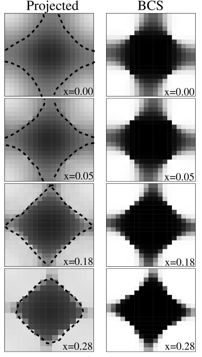
Figure 4: Grayscale plots (black $\equiv 1$, white $\equiv 0$) of the momentum distribution $n({\bf k})$ at various dopings $x$. The left panel shows the results of the projected variational calculation. The dashed line marks the contour on which $n({\bf k})=1/2$, which closely resembles the non-interacting Fermi surface. The right panel shows the $n({\bf k})$ of the unprojected BCS calculation at the corresponding doping value.

(3) Mott Insulator ($x=0$): At half-filling ($x=0$) $\Phi=0$ implying that the undoped state is nonsuperconducting. We will show below in Section X that its low frequency integrated optical spectral weight vanishes and thus it is an insulator.

A careful finite size scaling analysis of the spin structure factor shows that the $x=0$ is a critical state exhibiting algebraic decay of antiferromagnetic (AFM) spin correlations: $\langle S^{z}_{\bf{r}}S^{z}_{\bf 0}\rangle\sim(-1)^{r_{x}+r_{y}}/|{\bf{r}}|^{3/2}$. These results will be presented elsewhere paramekanti03 along with a detailed discussions of other competing order parameters at low doping.

The variational state at $x=0$ is an insulator made up of a superposition of singlet pairs: since ${\tilde{\Delta}}_{\rm var}(x=0)$ is nonzero, the function $\varphi({\bf{r}}-{\bf{r}^{\prime}})$ describes the singlet bonds in this state. The Gutzwiller projection prevents this liquid of singlet pairs from (super)conducting, and the $x=0$ state is an resonating valence bond (RVB) anderson87 or spin-liquid Mott insulator.

The form of the wavefunction studied here apparently does not have enough variational freedom to exhibit broken spin-rotational or translational invariance to describe the Neel AFM state which is known to be the experimental ground state of the undoped cuprate materials and also believed to be the ground state of the 2D large $U$ Hubbard model at half-filling. We plan to study in the future the competition between SC and AFM by adding more variational freedom in our trial state, but our primary focus here is a detailed characterization of the simplest description of a strongly-correlated superconducting state.

We should also note that the ground state energy of the our spin-liquid state at $x=0$ is within few percent of the best estimates. The best way to present this comparison to look at the spin correlation $\gamma\equiv\langle{\bf S}_{\bf{r}}\cdot{\bf S}_{\bf{r}^{\prime}}\rangle$ between neighboring sites ${\bf{r}}$ and ${\bf{r}^{\prime}}$ at half-filling. For our state we find $\gamma=-0.313\pm 0.002$. For comparison, the best estimate for the 2D nearest-neighbor Heisenberg model is $\gamma=-0.3346\pm 0.0001$ from Green’s function Monte Carlo calculations trivedi90 , while a classical Neel state has $\gamma=-0.25$. For the nearest neighbor hopping Hubbard model in the large $U$ limit, the ground state energy per site is $E_{0}=2J(\gamma-1/4)$ at half-filling. Further neighbor hopping leads to additive corrections of order $J^{\prime}/J=(t^{\prime}/t)^{2}=1/16$ for our choice of parameters.

V.3 Phase Transitions and Correlation Lengths

The variational wavefunction Eq. (5) describes the three phases discussed above, and our approach also gives interesting information about the quantum phase transitions between these phases. We find that there are diverging length scales in the SC state as one approaches the Mott insulator at $x=0$ and also the Fermi liquid metal beyond $x_{c}$.

The internal pair wavefunction $\varphi({\bf k})=v_{\bf k}/u_{\bf k}$, or more correctly the related quantity $v_{\bf k}u_{\bf k}$, defines a “pair-size” $\xi_{\rm pair}=\bar{v}^{0}_{F}/\Delta_{\rm var}$, where $\bar{v}^{0}_{F}$ is the bare average Fermi velocity. Projection is expected not to affect the pair-size much. $\xi_{\rm pair}$ diverges at $x_{c}$ and decreases monotonically with decreasing hole doping as the pairing becomes progressively stronger. The pair size remains finite at $x=0$, where it defines the range of singlet bonds in the RVB insulator, which is very short, of the order of the lattice spacing. Note that in converting the dimensionless ${\tilde{\Delta}}_{\rm var}$ to an energy (needed to define the pair size), we need to use the scale of either $t$ or $J$ (which we have chosen to be 300 and 100 meV respectively). In Section IX we will discuss this question in detail; here we simply chose $\Delta_{\rm var}=t{\tilde{\Delta}}_{\rm var}$, since in any case we want to get a lower bound on the coherence length.

A second important length scale is the average inter-hole spacing $1/\sqrt{x}$. At shorter distances there are no holes, no SC order can develop and the system effectively looks like the $x=0$ insulator. The SC correlation length $\xi_{\rm sc}$ must necessarily satisfy $\xi_{\rm sc}\geq\max\left(\xi_{\rm pair},1/\sqrt{x}\right)$. As shown in Fig. 3(b), this bound implies that $\xi_{\rm sc}$ must diverge both in the insulating limit $x\to 0$ and the metallic limit $x\to x_{c}^{-}$, but could be small (few lattice spacings) near optimal doping.

The divergence of $\xi_{\rm sc}(x)$ as $x\to 0$ could also be tested in experiments designed to measure the conductivity $\sigma({\bf{q}},\omega)$ in underdoped SC’s, at nonzero momentum ${\bf{q}}$. We expect significant ${\bf{q}}$-dependence at low $\omega$, with the conductivity rapidly vanishing for ${\bf{q}}>\xi_{\rm sc}^{-1}$ as insulating behavior is recovered. Another important question related to the proper definition of the correlation length concerns the vortex core radius as function of doping $x$. This problem deserves careful study using Gutzwiller wavefunctions, since the $U(1)$ slave boson-gauge theory approach predicts that the vortex core size diverges as $1/\sqrt{x}$ as $x\to 0$ dhlee , while an SU(2) approach palee97 suggests a stronger $1/x$ divergence.

It is clear that we must carefully distinguish between various “coherence lengths”, which are the same in simple BCS theory up to factors of order unity, but could be very different in strongly correlated SCs. Only the result of a detailed calculation can reveal which coherence length is relevant for a particular experiment.

Figure 5: Schematic plot of the spectral function when gapless quasiparticles are dispersing across the chemical potential, $\omega=0$, with a quasiparticle weight $Z$ and velocity $v_{{}_{F}}$. The solid (dashed) lines indicate the occupied (unoccupied) part of the spectral function.

VI Momentum Distribution

Next we study the momentum distribution $n({\bf k})=\langle c^{\dagger}_{{\bf k}\sigma}c_{{\bf k}\sigma}\rangle$. This is calculated by computing the Fourier transform of $\langle{\cal G}_{\sigma}({\bf{r}},{\bf{r}^{\prime}})\rangle\equiv\langle c^{\dagger}_{{\bf{r}}\sigma}c_{{\bf{r}^{\prime}}\sigma}\rangle$. The details of the transformed operator $\tilde{\cal G}=\exp(iS){\cal G}\exp(-iS)$ to first order in $t/U$ are given in Appendix A.

In Fig. (4) (left panel) we show grayscale plots of $n({\bf k})$ at various doping values ranging from the insulating state at $x=0$ to the overdoped SC at $x=0.28$. We see that $n({\bf k})$ has considerable structure at all dopings including $x=0$. These results are qualitatively consistent with photoemission experiments on the SC cuprates ding97 ; fujimori00 and related insulating compounds ronning98 .

In a strict sense there is no meaning to a Fermi surface (FS) at $T=0$ since the system is either SC or insulating (at $x=0$) for $0\leq x<x_{c}$. Nevertheless it is interesting to note that if one plots either the contour on which $n({\bf k})=1/2$ (shown as a dashed line in Fig. (4)) or the contour on which $|\nabla_{\bf k}n({\bf k})|$ is maximum (not shown), both are very similar to the noninteracting FS that would have been obtained from the free dispersion $\epsilon({\bf k})$. For this reason we call such contours the interacting “Fermi surface” mesot01 . These similarity between the interacting and non-interacting FS is closely related to the approximate equality of $\mu_{\rm BCS}$ and the variational parameter $\mu_{\rm var}$ discussed in Sec. IIIB.

To further see the extent to which strong correlations affect the momentum distribution, we compare the $n({\bf k})$ obtained from the projected wavefunctions in the left panel with that obtained from simple BCS theory. The BCS result $n({\bf k})=v_{\bf k}^{2}$ using optimal values ${\tilde{\Delta}}_{\rm var}$ and ${\tilde{\mu}}_{\rm var}\simeq\mu_{\rm BCS}/t$ is plotted in the right panel of Fig. (4). While projection leads to a transfer of spectral weight (i.e., $n({\bf k})$ intensity) from the zone center to the zone corners, the overall “topology” of the momentum distribution is not qualitatively changed.

For $t^{\prime}=t/4$, the noninteracting FS and the interacting “FS” both show a change in topology from a large hole-like barrel centered at $(\pi,\pi)$ for small $x$ to an electron-like FS for $x\gtrsim 0.22$. The precise value at which the topology changes depends sensitively on the sign and value of $t^{\prime}$. Such a topology change has been clearly observed in ARPES data on LSCO fujimori00 and less obviously in BSCCO where the topology change may be happening at large overdoping jc_private .

In later sections we will return to a detailed study of $n({\bf k})$ along special directions in the Brillouin zone, where we will see that strong correlations play a crucial role, even though they appear to be not very important in so far as gross features like the topology of the “Fermi surface” is concerned.

Figure 6: (a),(b) The momentum distribution, $n({\bf k})$, along the nodal direction $(0,0)\to(\pi,\pi)$ (black squares). The white squares are results for the tJ model, and correspond to ignoring $t/U$ corrections in Eq. (24). The nonmonotonic behavior of $n({\bf k})$ near $k_{{}_{F}}$ is removed on including ${\cal O}(t/U)$ terms. The discontinuity in $n({\bf k})$ at $k=k_{{}_{F}}$ signals gapless quasiparticles with a weight $Z$ determined by the magnitude of the jump. (c) Doping dependence of $Z$ compared with $Z^{\rm sb}=x$ from slave-boson mean-field theory.

VII Spectral Function Moments

A variational wave function approach is limited to the calculation of equal-time correlations and thus interesting dynamical information would, at first sight, seem to be out of reach. We now show that this is not always true. First, the frequency moments of dynamical correlations can always be written as equal-time correlators, and this in itself can give very useful information as we shall see in the following sections. Further, one can obtain much more detailed information, when the moments, which are functions only of ${\bf k}$ with $\omega$ integrated out, exhibit singularities in ${\bf k}$. In the case of the single-particle Green’s function, we show that the singularities of its moments at $T=0$ are completely governed by gapless quasiparticles, if they exist.

The one-particle spectral function is defined in terms of the retarded Green function as $A({\bf k},\omega)=-{\rm Im}G({\bf k},\omega+i0^{+})/\pi$, and has the $T=0$ spectral representation

$$A({\bf k},\omega) = \sum_{m}\big{[}|\langle m|c_{{\bf k}\sigma}^{\dagger}|0\rangle|^{2}\delta(\omega+\omega_{0}-\omega_{m})$$ (8)

$$+ |\langle m|c_{{\bf k}\sigma}|0\rangle|^{2}\delta(\omega-\omega_{0}+\omega_{m})\big{]}.$$

Here $|m\rangle$ (and $\omega_{m}$) are the eigenstates (and eigenvalues) of $({\cal H}-\mu N)$ with $N$ the total number of particles and all energies are measured with respect to $\mu$.

One can consider moments of the full spectral function white91 , but for our purposes it is much more useful to consider moments of the occupied part of spectral function $f(\omega)A({\bf k},\omega)$, where $f(\omega)$ is the Fermi function. This is also the quantity measured in ARPES experiments randeria95 . At $T=0$, $f(\omega)=\Theta(-\omega)$ and only the second term in the spectral representation contributes: $\Theta(-\omega)A({\bf k},\omega)=|\langle m|c_{{\bf k}\sigma}|0\rangle|^{2}\delta(\omega-\omega_{0}+\omega_{m})$.

The $\ell^{\rm th}$ moment of the occupied spectral function $M_{\ell}({\bf k})\equiv\int_{-\infty}^{0}d\omega\omega^{\ell}A({\bf k},\omega)$ can be expressed as a ground state correlator following standard algebra. We will focus on the first two moments in what follows. These are given by:

$$M_{0}({\bf k})=\int_{-\infty}^{0}d\omega A({\bf k},\omega) = \sum_{m}|\langle m|c_{{\bf k}\sigma}|0\rangle|^{2}=n({\bf k})$$

$$M_{1}({\bf k})=\int_{-\infty}^{0}d\omega\omega A({\bf k},\omega) = \sum_{m}(\omega_{0}-\omega_{m})|\langle m|c_{{\bf k}\sigma}|0\rangle|^{2}$$ (9)

$$= \langle c_{{\bf k}\sigma}^{\dagger}\big{[}c_{{\bf k}\sigma},{\cal H-\mu N}\big{]}\rangle$$

$$= \langle c_{{\bf k}\sigma}^{\dagger}\big{[}c_{{\bf k}\sigma},{\cal H}\big{]}\rangle-\mu n({\bf k})$$

We next describe the characteristic singularities in these moments arising from coherent quasiparticle (QP) excitations; the result for the momentum distribution is very well known, but that for the first moment seems not to have been appreciated before. In the presence of gapless quasiparticles, the spectral function has the form

$$A({\bf k},\omega)=Z\delta(\omega-\tilde{\xi}_{\bf k})+A_{\rm inc}({\bf k},\omega),$$ (10)

plotted schematically in Fig. (5). Here $Z$ is the coherent QP weight $(0<Z\leq 1)$ and $\tilde{\xi}_{{\bf k}}=v_{{}_{F}}(k-k_{{}_{F}})$ is the QP dispersion with $k_{{}_{F}}$ the Fermi wavevector and $v_{{}_{F}}$ the Fermi velocity. $A_{\rm inc}({\bf k},\omega)$ is the smooth, incoherent part of the spectral function. It is then easy to see from Eq. (9) that

$$M_{0}({\bf k}) = n({\bf k})=Z\theta(-\tilde{\xi}_{\bf k})+\ldots$$

$$M_{1}({\bf k}) = Z\tilde{\xi}_{\bf k}\theta(-\tilde{\xi}_{\bf k})+\ldots,$$ (11)

where the terms omitted are the non-singular contributions from the incoherent piece.

It follows that, precisely at $k=k_{{}_{F}}$, $M_{0}({\bf k})$ has a jump discontinuity of $Z$ and $dM_{1}({\bf k})/dk$ has a discontinuity of $Zv_{{}_{F}}$. Thus, studying the moments of $\Theta(-\omega)A({\bf k},\omega)$ allows us to extract $Z$ and $v_{{}_{F}}$ from singular behavior of $M_{0}({\bf k})$ and $M_{1}({\bf k})$, while $k_{{}_{F}}$ can be determined from the location in ${\bf k}$-space where this singularity occurs.

It is worth emphasizing what has been achieved. In strongly correlated systems, interactions lead to a transfer of spectral weight from coherent excitations to incoherent features in the spectral function. The values of $M_{\ell}({\bf k})$ are, in general, dominated by these incoherent features (which we will find to be very broad in the cases we examine), but nevertheless their singularities are governed by the gapless coherent part of the spectral function, if it exists. We exploit these results below in our study of nodal quasiparticles in the d-wave SC state.

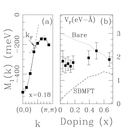
Figure 7: (a) The first moment of the occupied part of the spectral function $M_{1}({\bf k})$ along the zone diagonal $(0,0)\to(\pi,\pi)$ showing discontinuity of $Zv_{{}_{F}}$ in its slope, $dM_{1}({\bf k})/dk$, at $k=k_{{}_{F}}$. (b) Doping dependence of $v_{{}_{F}}$, extracted from $M_{1}({\bf k})$. The error bars here are associated with fits to $M_{1}({\bf k})$ and $n({\bf k})$ and errors in $Z$. Also shown are the bare velocity $v^{0}_{{}_{F}}$ (dashed line) and the QP velocity within slave-boson mean-field theory, $v_{{}_{F}}^{\rm sb}$ (dotted line). The experimental QP velocity $\simeq 1.5eV\stackrel{{{}_{~{}\circ}}}{{\textstyle A}}$ from ARPES datakaminski in near optimal BSCCO, and experiments indicate that it is nearly doping independent .nodalQPpaper

VIII Nodal quasiparticles

There is considerable evidence from ARPES kaminski ; valla99 ; bogdanov00 and transport experiments hardy93 ; ong95 ; taillefer00 that there are sharp gapless quasiparticle (QP) excitations in the low temperature superconducting state along the nodal direction $(0,0)\to(\pi,\pi)$. These nodal excitations then govern the low temperature properties in the SC state. In this section we show that our SC wavefunction supports sharp nodal quasiparticles and calculate various properties such as their location $k_{{}_{F}}(x)$, spectral weight $Z(x)$ and Fermi velocity $v_{{}_{F}}(x)$ as a function of doping and compare with existing experiments.

VIII.1 $k_{{}_{F}}(x)$ and $Z(x)$

In Figs. 6(a) and (b) we plot the momentum distribution (black squares) $n({\bf k})$ along $(0,0)\to(\pi,\pi)$ for two different doping levels. We see a clear jump discontinuity which implies the existence of sharp, gapless nodal QPs. (Note that such a discontinuity is not observed along any other direction in ${\bf k}$-space due to the existence of a d-wave SC gap.) We thus determine the nodal $k_{F}(x)$, the location of the discontinuity in $n({\bf k})$, and the nodal QP weight $Z$ from the magnitude of the jump in $n({\bf k})$ footnote_z .

We find that the nodal $k_{F}(x)$ has weak doping dependence consistent with ARPES ding97 ; fujimori00 , and at optimal doping $k_{{}_{F}}\approx 0.69\stackrel{{{}_{~{}\circ}}}{{\textstyle A}}^{-1}$, which is close to the ARPES value of $0.707\stackrel{{{}_{~{}\circ}}}{{\textstyle A}}^{-1}$ mesot99 . As already noted while discussing Fig. (4), $k_{{}_{F}}$ is not much affected by interaction and noninteracting (band theory) estimates for $k_{{}_{F}}$ are accurate.

In contrast, we find that interactions have a very strong effect on coherence: the QP spectral weight $Z$ is considerably reduced from unity and the incoherent weight $(1-Z)$ is spread out to high energies. We infer large incoherent linewidths from the fact that, even at the zone center ${\bf k}=(0,0)$ which is the “bottom of the band” $n({\bf k}=(0,0))\simeq 0.85$ (for $x=0.05$), implying that 15% of the spectral weight must have spilled over to the unoccupied side $\omega>0$. A second indicator of large linewidths is the magnitude of the first moment discussed below.

The doping dependence of the nodal QP weight $Z(x)$ is shown in Fig. 6(c). The most striking feature is the complete loss of coherence as $x\to 0$, with $Z\sim x$ as the insulator is approached. We can understand the vanishing of $Z(x)$ as $x\to 0$ from the following argument. A jump discontinuity in $n({\bf k})$ leads to the following long distance behavior in its Fourier transform ${\cal G}({\bf{r}})=\langle c^{\dagger}_{\sigma}({\bf{r}})c_{\sigma}(0)\rangle$: a power law decay with period $k_{{}_{F}}^{-1}$ oscillations and an overall amplitude of $Z$. However, for ${\cal G}({\bf{r}})$ to be nonzero at large $r$ in a projected wavefunction, we need to find a vacant site at a point $|{\bf{r}}|$ away from the origin. This probability scales as $x$, the hole density, and thus $Z\sim x$. Near half-filling we expect this $x$-dependence due to projection to dominate other sources of $x$-dependence footnote_log , in the same way as the discussion of the order parameter $\Phi(x)$ (see Sec. V.B) and we see why $Z\sim x$ for $x\ll 1$.

After our theoretical prediction paramekanti01 of the nodal QP $Z(x)$, ARPES studies on La_2-xSr_xCuO₄ (LSCO) yoshida02 have been used to systematically extract the nodal $Z$ as a function of Sr concentration $x$. The extracted $Z$’s are in arbitrary units, but the overall trend, and particularly the vanishing of $Z$ as $x\to 0$, is roughly consistent with our predictions. We should note however that underdoped LSCO likely has a strong influence of charge and spin ordering competing with the superconductivity. While this physics is not explicitly built into our wavefunction, the vanishing of $Z$ with underdoping is a general property of projected states as discussed above.

We next contrast our results with those obtained for similar variational calculation on the tJ model, which gives insight into the differences between the large $U$ Hubbard (black squares) and tJ models (open symbols in Figs. 6(a) and (b)). The tJ model results, which set $\exp(iS)=1$ in so far as the operator $c^{\dagger}_{\sigma}({\bf{r}})c_{\sigma}(0)$ is concerned, lead to an $n({\bf k})$ which is a non-monotonic function of ${\bf k}$. This is somewhat unusual, although not forbidden by any exact inequality or sum rule. Further, the tJ model $n({\bf k})$ is a ${\bf k}$-independent constant equal to one-half at $x=0$. However, we find that the $t/U$ corrections incorporated in the $\exp(iS)$ factor in the Hubbard model, which arise from mixing in states with double occupancy into the ground state, lead to a nontrivial structure in $n({\bf k})$ at all $x$ including $x=0$ and also eliminate the nonmonotonic feature near $k_{{}_{F}}$. At $x=0$ (see Eq. (29) in Appendix B) the $t/U$ corrections arise from short-range antiferromagnetic spin correlations. These correlations are expected to persist even away from half-filling although they get weaker with increasing $x$.

Finally we compare our result for $Z(x)$ with that obtained from slave boson mean field theory (SBMFT). In Fig. 6(c), we also plot the SBMFT result $Z^{\rm sb}=x$ and find $Z(x)>Z^{\rm sb}(x)$, i.e., the SBMFT underestimates the coherence of nodal QPs. To understand the significance of this difference, we must look at the assumptions of SBMFT. (1) There is a full “spin-charge separation”, so that that the spinon and holon correlators completely decouple, i.e., factorize. (2) There is complete Bose condensation of the holons: $|\langle b\rangle|^{2}=x$. (3) The spinon momentum distribution corresponds to that of a mean-field d-wave BCS SC with a jump $Z_{\rm sp}=1$ along the nodal direction. With these assumptions, the jump in $n({\bf k})$ is just given by $Z^{\rm sb}=|\langle b\rangle|^{2}Z_{\rm sp}=x$. Conditions (2) and (3) are definitely violated as one goes beyond the mean field approximation. However, we then expect $|\langle b\rangle|^{2}<x$ and $Z_{\rm sp}<1$ both of which lead to a further decrease in $Z^{\rm sb}$. Thus the observed inequality $Z(x)>Z^{\rm sb}(x)$ implies that assumption (1) must also be violated when the constraint is taken into account by including gauge fluctuations around the SBMFT saddle point. Inclusion of such gauge fluctuations would also be necessary to obtain the incoherent part of the spectral function. We thus conclude that the spinons and holons of SBMFT must be strongly interacting and their correlator cannot be factorized.

VIII.2 Nodal quasiparticle velocity $v_{{}_{F}}(x)$

The first moment $M_{1}({\bf k})$ of the occupied part of $A({\bf k},\omega)$ is plotted in Fig. 7(a) as a function of ${\bf k}$ long the zone diagonal $(0,0)\to(\pi,\pi)$. We note that, even at $k_{{}_{F}}$, the moment $M_{1}(k_{{}_{F}})$ lies significantly below $\omega=0$: for $x=0.18$ it is $200$ meV below the chemical potential. This directly quantifies the large incoherent linewidth alluded to earlier.

We have already established the existence of nodal quasiparticles, so they must lead to singular behavior in $M_{1}({\bf k})$ with a slope discontinuity of $Zv_{F}$ at $k_{F}$. We can see this clearly in Fig. 7(a) and use this to estimate the nodal Fermi velocity $v_{{}_{F}}$, whose doping dependence is plotted in Fig. 7(b). The large error bars on the $v_{{}_{F}}$ estimate come from the errors involved in extracting the slope discontinuity in $M_{1}({\bf k})$.

First, we see that $v_{{}_{F}}(x)$ is reduced by almost a factor of two relative to its bare (band structure) value $v^{0}_{{}_{F}}$ in the low doping regime of interest, which corresponds to a mass-enhancement due to interactions. At large $x\geq 0.5$, deep in the Fermi liquid regime, the $v_{{}_{F}}$ obtained from the moment calculation agrees with the bare velocity, which also serves as a nontrivial check on our calculation.

More remarkably, we see that the renormalized $v_{{}_{F}}(x)$ is essentially doping independent in the SC part of the phase diagram, and appears to remain finite as $x\to 0$. Thus, as one approaches the insulator at $x=0$, the coherent QP weight vanishes like $Z\sim x$, but the effective mass $m^{\ast}$ remains finite. This has important implications for the form of the nodal quasiparticle self-energy which are discussed in detail below. The value and the weak doping dependence of the nodal Fermi velocity are both consistent with the ARPES estimatekaminski of $v_{F}\approx 1.5eV$-$\stackrel{{{}_{~{}\circ}}}{{\textstyle A}}$ in Bi₂Sr₂CaCu₂O_8+δ (BSCCO). Very recently, our prediction has been tested by ARPES experiments on LSCO zhou03 , where a remarkably doping independent (low energy) $v_{F}$ has been found.

It is also instructive to compare this result with the the SBMFT result $v^{\rm sb}_{{}_{F}}$ (dashed line in Fig. 7(b)) obtained from the spinon dispersion as discussed in Appendix C. We find that $v^{\rm sb}_{{}_{F}}$ is much less than $v_{{}_{F}}$ and has considerable doping dependence, even though SBMFT does predict a nonzero $v^{\rm sb}_{{}_{F}}$ as $x\to 0$. Thus not only do the nodal QPs have more coherence than in SBMFT, they also propagate faster.

Another important nodal quasiparticle parameter is the “gap velocity” $v_{2}\equiv{1\over k_{F}}\partial\Delta(\theta)/\partial\theta|_{\theta=\pi/4}$, which is the slope of the SC energy gap at the node ($\theta=\pi/4$ in the first quadrant of the Brillouin zone). Together with $k_{{}_{F}}$ and $v_{{}_{F}}$, $v_{2}$ completely specifies the Dirac cone for the nodal QP dispersion: $E({\bf k})=\sqrt{(v_{{}_{F}}k_{\perp})^{2}+(v_{2}k_{\parallel})^{2}}$, where $k_{\perp}$ ($k_{\parallel}$) are the deviations from $k_{{}_{F}}$ perpendicular (parallel) to the Fermi surface. In a d-wave SC one expects the singular part of $A({\bf k},\omega)\Theta(-\omega)$ to be of the form $Zv_{\bf k}^{2}\delta(\omega+E({\bf k}))$ near the node. Thus the singular part of the first moment $M_{1}({\bf k})$ is given by $-Z\left[E({\bf k})-v_{{}_{F}}k_{\perp}\right]/2$. For $k_{\parallel}=0$ (i.e., ${\bf k}$ along the zone diagonal) this simply reproduces the slope discontinuity analyzed above. However, setting $k_{\perp}=0$, one finds $M_{1}({\bf k})=-Zv_{2}|k_{\parallel}|/2+{\rm smooth}$, so that crossing the node by moving along the Fermi surface, one would see a slope discontinuity in $M_{1}({\bf k})$ from which $v_{2}$ may be estimated, in principle.

In practice, we are unable to extract this singularity from our present calculations owing to two difficulties. First, one requires a dense sampling of ${\bf k}$-points lying on the Fermi surface, which cannot be achieved for accessible system sizes which are limited by the computational time. Second, it is known from experiments mesot99 ; taillefer00 that $v_{{}_{F}}/v_{2}\gg 1$ (around $15$ to $20$); thus small errors in locating the Fermi surface would mean that the $M_{1}({\bf k})$ would be dominated by effects of $v_{{}_{F}}$. Nevertheless, it would be very interesting to calculate $v_{2}$ in the future.

VIII.3 Nodal quasiparticle self-energy

The doping dependence of nodal QP spectral weight $Z(x)$, and Fermi velocity $v_{{}_{F}}(x)$ obtained above, places strong constraints on the self-energy $\Sigma({\bf k},\omega)$ particularly near the SC to insulator transition as $x\to 0$. For ${\bf k}$ along the zone diagonal $(0,0)\to(\pi,\pi)$ the gap vanishes in a d-wave SC and ignoring the off-diagonal self-energy we can simply write the Green function as $G^{-1}({\bf k},\omega)=\omega-\epsilon({\bf k})-\mu-\Sigma({\bf k},\omega)$, where $\Sigma\equiv\Sigma^{\prime}+\Sigma^{\prime\prime}$. Standard arguments then lead to the results

$$Z = \left(1-\frac{\partial\Sigma^{\prime}}{\partial\omega}\right)^{-1}$$

$$v_{{}_{F}} = Z\left(v_{{}_{F}}^{0}+\frac{\partial\Sigma^{\prime}}{\partial k}\right)$$ (12)

where the right hand side is evaluated at the node $(k_{{}_{F}},\omega=0)$.

From $Z\sim x\to 0$ we conclude that $|\partial\Sigma^{\prime}/\partial\omega|$ diverges like $1/x$ as $x\to 0$. However since $v_{{}_{F}}$ remains finite in this limit, there must be a compensating divergence in the ${\bf k}$-dependence of the self-energy with $\partial\Sigma^{\prime}/\partial k\sim 1/x$. A similar situation is also realized in the slave-boson mean-field solution discussed in Appendix C, even though it is quantitatively a poor description of the results for $Z(x)$ and $v_{{}_{F}}(x)$. The first example we are aware of where such compensating divergences appeared is the normal Fermi liquid to insulator transition in the large-$N$ solution of the tJ model kotliar.largeN .

Note that the results obtained here are very different from many other situations where the self energy has non-trivial $\omega$ dependence, but is essentially ${\bf k}$-independent. These include examples as diverse as electron-phonon interaction, heavy fermions heavyfermion (where the large $m^{\ast}$ or small $v_{{}_{F}}$ is tied to a small $Z$), and the Mott transition in dynamical mean field theory kotliar96 .

Figure 8: The dimensionless variational parameter $\Delta_{\rm var}(x)$ of Fig. 1(a) is converted to an energy scale $\alpha J\Delta_{\rm var}(x)$, where $\alpha$ is a dimensionless prefactor of order unity. The corresponding energy scale (in meV) is plotted as a function of hole-doping $x$. For the choice $\alpha=0.8$ the energy scale (filled circles) agrees well with the ARPES energy gap in the SC state (open hexagons), while for $\alpha=3$ it (filled squares) agrees well with the “hump” scale (open triangles) in ARPES spectra at ${\bf k}=(\pi,0)$. All the ARPES results are taken from Campuzano et al. campuzano99 .

IX Spectral function along $(\pi,0)\to(\pi,\pi)$

We now move away from the zone diagonal and examine the neighborhood of ${\bf k}=(\pi,0)$, where the anisotropic d-wave SC gap is the largest. Our main aim is to see if we can learn something the spectral gap and its doping dependence. The information available from ground state correlation functions is not sufficient to rigorously estimate the excitation gap, so we proceed in two different ways using some guidance from experiments. First, we convert our dimensionless variational parameter ${\tilde{\Delta}}(x)_{\rm var}$ to an energy scale and compare with experiment, and second, we use the information available from the moments $n({\bf k})$ and $M_{1}({\bf k})$ along $(\pi,0)$ to $(\pi,\pi)$.

As discussed above, the superexchange interaction scale $J$ leads to pairing, and in addition as one approaches the insulator at $x=0$, $J$ is the only scale in the problem. In view of this it is natural to consider $J{\tilde{\Delta}}_{\rm var}(x)$ as the energy scale characteristic of pairing. In Fig. 8 we plot $\alpha J{\tilde{\Delta}}_{\rm var}(x)$ as function of the hole doping $x$ where $\alpha$ is a dimensionless number of order unity. For the choice $\alpha=0.8$ we find that we get very good agreement with the experimentally measured values and doping dependence of the energy gap as obtained from ARPES campuzano99 .

Figure 9: (a) The momentum distribution $n({\bf k})$ along the $(\pi,0)\to(\pi,\pi)$ direction, compared with the unprojected BCS result at the same ${\tilde{\Delta}}_{\rm var}$ and $\mu_{\rm var}$. These results imply that correlations leads to considerable broadening of $n({\bf k})$. (b) $n({\bf k})$ plotted for various $x$, showing increasing broadening as $x\to 0$, induced by correlations.

Next we use the spectral function moments $n({\bf k})$ and $M_{1}({\bf k})$ to get further insights into the pairing scale. In the presence of a gap there are no singularities in the moments and hence we cannot directly hope to get information about the coherent part of the spectral function, as we did near the nodes. However, as argued below, we will use the moments to determine a characteristic energy scale for the incoherent part of the spectral function, which we are able to relate, on the one hand, to the variational parameter ${\tilde{\Delta}}_{\rm var}(x)$ and, on the other, to the experimentally observed $(\pi,0)$ hump scale in ARPES campuzano99 .

The ratio of the first moment to the zeroth moment of the occupied spectral function

$$|M_{1}({\bf k})|/n({\bf k})={{\int d\omega\omega f(\omega)A({\bf k},\omega)}\over{\int d\omega f(\omega)A({\bf k},\omega)}}\equiv\langle\omega\rangle({\bf k}),$$ (13)

naturally defines a characteristic energy scale $\omega\rangle({\bf k})$. Before studying this quantity in detail, it may help to first look at each of the moments individually as a function of doping.

From Fig. 9(a) we see that the momentum distribution $n({\bf k})$ for the projected ground state is much broader along $(\pi,0)\to(\pi,\pi)$ compared with that for the unprojected $|\Psi_{\rm BCS}\rangle$ with the same ${\tilde{\Delta}}_{\rm var}$. This suggests that it is not the energy gap, but rather the correlation-induced incoherence in the spectral functions, that is broadening $n({\bf k})$. A direct measure of the incoherent linewidth in terms of the first moment $M_{1}({\bf k})$ will be discussed below. We see that projection leads to a significant build up of spectral weight for ${\bf k}$’s in the range $(\pi,0.2\pi)$ to $(\pi,\pi)$, which were essentially unoccupied in the unprojected $|\Psi_{\rm BCS}\rangle$ state. Correspondingly, correlations lead to a loss of spectral weight near $(\pi,0)$. The doping dependence of $n({\bf k})$ for the projected ground state is shown in Fig. 9(b). The increasing importance of correlations with underdoping is evident from the fact that $n({\bf k})$ becomes progressively broader with decreasing $x$.

In Fig. 10(a), we plot the first moment of the occupied part of the spectral function $M_{1}({\bf k})$ along $(\pi,0)\to(\pi,\pi)$ and compare it with the unprojected BCS value. We find that correlations lead to a large negative value of $M_{1}({\bf k})$ which indicates a large incoherent spectral linewidth.

The quantity $\langle\omega\rangle({\bf k})$, defined by the ratio of moments in eq. (13), is the characteristic energy scale over which the occupied spectral weight is distributed. Quite generally we expect this to be dominated by the large incoherent part of the spectral function. We see from Fig. 10(b) that this energy scale at $(\pi,0)$ increases with underdoping. This trend arises from a combination of an increasing spectral gap and an increasing incoherent linewidth at ${\bf k}=(\pi,0)$ as $x\to 0$.

It can be argued that the energy $\langle\omega\rangle(\pi,0)$ is an upper bound on the SC gap, even though a very crude (i.e., inaccurate) one. This can be seen by using $c_{{\bf k}\sigma}|\Psi_{0}\rangle$ as a trial excited state. A more sensible trial state is obtained by projecting a Bogoliubov quasiparticle state (where the excitation is created first and then projected, unlike the above case where this order is reversed). This and further improved excited states are currently under investigation and will be discussed in a later publication.

From Fig. 10(b) we see that, as a function of doping, the energy $\langle\omega\rangle(\pi,0)$ scales linearly with the variational parameter ${\tilde{\Delta}}_{\rm var}(x)$, characterizing pairing in the wavefunction. This suggests that we should think of ${\tilde{\Delta}}_{\rm var}$ as a characteristic incoherent scale in the SC state $A({\bf k},\omega)$ at $(\pi,0)$. A second argument in support of such an identification comes from the observation that at and near $x=0$ ${\tilde{\Delta}}_{\rm var}$ is mainly determined by minimizing the exchange energy. This implies a close relation between local antiferromagnetic order and short-range d-wave singlet pairing. This is directly borne out by correlating the doping dependences of ${\tilde{\Delta}}_{\rm var}$ and the near-neighbor spin correlation (which will be described in detail elsewhere). All of these arguments serve to relate ${\tilde{\Delta}}_{\rm var}$ to high energy, short-distance physics, rather than to the low energy coherent feature such as the quasiparticle gap in the SC state.

Figure 10: (a) The first moment of the occupied part of the spectral function $M_{1}({\bf k})$ along the $(\pi,0)\to(\pi,\pi)$ direction compared with the corresponding unprojected BCS result. $|M_{1}({\bf k})|$ is much larger than the BCS result from which we infer that strong correlations lead to very large incoherent linewidth. (b) Parametric plot of $\langle\omega\rangle({\bf k})\equiv|M_{1}({\bf k})|/n({\bf k})$ (see text) at ${\bf k}=(\pi,0)$. versus ${\tilde{\Delta}}_{\rm var}$ with doping $x$ as the implicit parameter. The linear relation indicates that ${\tilde{\Delta}}_{\rm var}(x)$ is related to an incoherent energy scale in the spectral function at $(\pi,0)$.

Motivated by these arguments we compare the energy scale obtained from the variational parameter $\alpha J{\tilde{\Delta}}_{\rm var}(x)$ with an experimentally observed incoherent scale in the SC spectral function at $(\pi,0)$. The natural candidate for the latter is the $(\pi,0)$ “hump” in ARPES, where it has been established that the spectral function at $(\pi,0)$ has a very interesting peak-dip-hump structure for $T\ll T_{c}$ at all dopings campuzano99 . The sharp peak corresponds to the coherent quasiparticle at the SC energy gap, while “hump” comes from the incoherent part of the spectral function. Two other significant experimental facts about the hump are that: (a) While both the hump and gap energies decrease monotonically with hole doping $x$, their ratio is roughly doping independent, with the hump being a factor of $3.5$ to $4.0$ larger than the SC gap campuzano99 . (b) A vestige of the hump persists even above $T_{c}$ on the underdoped side where it is called the “high energy pseudogap” campuzano03 .

In Fig. 8, we find good agreement between the energy scale $\alpha J{\tilde{\Delta}}_{\rm var}(x)$ with the ARPES $(\pi,0)$ hump energy measured by Campuzano and coworkers campuzano99 , provided we choosefootnote.oldpaper $\alpha=3$. In summary, with one choice of $\alpha$ ($=0.8$) we find good agreement with the experimentally observed energy gap and with another choice of $\alpha$ ($=3.0$) we find good agreement with the ARPES hump scale. We hope that in the future a study of variational excited states will give a direct estimate of the energy gap and also explain the ratio of approximately $3.75$ (independent of $x$) between the hump and gap.

Figure 11: (a): Doping dependence of the total ($D_{\rm tot}$) and Drude or low energy ($D_{\rm low}$) optical spectral weights. $D_{\rm low}\sim x$ at low $x$, which implies a Mott insulating state at $x=0$. (b): Parametric plot of the Drude weight $D_{\rm low}$ versus the nodal quasiparticle weight $Z$, with hole doping $x$ as the implicit parameter. We find $D_{\rm low}\sim Z$ over $0<x<x_{c}$.

X Optical sum rules and superfluidity

X.1 Total and low energy optical spectral weights

We next turn to a discussion of the optical conductivity. For a superconductor the real part of the optical conductivity is of the form $\sigma(\omega)=\pi e^{2}D_{s}\delta(\omega)+\sigma_{\rm reg}(\omega)$, where the condensate contributes the $\delta(\omega)$ whose strength is the superfluid stiffness $D_{s}$, while the regular part $\sigma_{\rm reg}(\omega)$ comes from excitations. We will now exploit sum rules which relate frequency integrals of $\sigma(\omega)$ to equal time ground state correlation functions which can be reliably calculated in our formalism.

For a single-band model, the optical conductivity sum rule scalapino93 ; paramekanti00 can be written as

$$\int_{0}^{\infty}d\omega Re\sigma(\omega)=\pi\sum_{{\bf k}}m^{-1}({\bf k})n({\bf k})\equiv\pi D_{\rm tot}/2$$ (14)

where $m^{-1}({\bf k})=$ $\left(\partial^{2}\epsilon({\bf k})/\partial{\bf k}_{x}\partial{\bf k}_{x}\right)$ is the noninteracting inverse mass and we set $\hbar=c=e=1$. All effects of interactions enter through the momentum distribution $n({\bf k})$.

The total optical spectral weight $D_{\rm tot}(x)$ plotted in Fig. 11(a) is found to be non-zero for $x=0$ and an increasing function of hole concentration $x$ in the regime shown. We have also found that $D_{\rm tot}$ decreases for $x>0.4$ and eventually vanishes at $x=1$, as it must in the empty band limit. These results, which are not shown here, serve as a nontrivial check on our calculation.

It is more important for our present purposes to understand why the total optical spectral weight in the insulating limit ($x=0$) is non-zero. This is because the infinite cutoff in the above integral includes contributions due to transitions from the ground state to the “upper Hubbard band”, i.e., to states with doubly occupied sites whose energies $\omega\gtrsim U$.

A physically much more interesting quantity is the low frequency optical weight $D_{\rm low}$, often called the Drude weight, where the upper cutoff in Eq. (14) is chosen to be $\Omega_{c}$ such that $J\leq t\ll\Omega_{c}\ll U$. The question then arises: can one write $D_{\rm low}$ as an equal-time correlation? Toward this end it is convenient to work in the “low energy” basis, using the ground state wavefunction ${\cal P}|\Psi_{\rm BCS}\rangle$, and explicitly include the canonical transformation $\exp(-iS)$ on the operators. In the presence of a vector potential, the canonically transformed Hamiltonian (see Appendix A) to ${\cal O}(t^{2}/U)$ is given by

$$\tilde{{\cal H}}_{A} = \sum_{{\bf{r}}{\bf{r}^{\prime}}\sigma}t_{{\bf{r}}{\bf{r}^{\prime}}}e^{iA_{{\bf{r}}{\bf{r}^{\prime}}}}\big{[}h_{{\bf{r}}{\bar{\sigma}}}c_{{\bf{r}}\sigma}^{{\dagger}}c_{{\bf{r}^{\prime}}\sigma}h_{{\bf{r}^{\prime}}{\bar{\sigma}}}\big{]}$$ (15)

$$- \frac{1}{U}\sum_{{\bf{r}}{\bf{r}^{\prime}}{\bf R}\sigma{\sigma^{\prime}}}t_{{\bf{r}}{\bf R}}t_{{\bf R}{\bf{r}^{\prime}}}e^{i\left(A_{{\bf{r}}{\bf R}}+A_{{\bf R}{\bf{r}^{\prime}}}\right)}h_{{\bf{r}}{\bar{\sigma}}}c_{{\bf{r}}\sigma}^{{\dagger}}c_{{\bf R}\sigma}n_{{\bf R}{\bar{\sigma}}}$$

$$\times c_{{\bf R}{\sigma^{\prime}}}^{{\dagger}}c_{{\bf{r}^{\prime}}{\sigma^{\prime}}}h_{{\bf{r}^{\prime}}{\bar{\sigma}^{\prime}}}.$$

This can be used to extract the diamagnetic response operator $\tilde{{\cal D}}_{\rm dia}\equiv\partial^{2}\tilde{\cal H}_{A}/\partial A^{2}$

$$\tilde{{\cal D}}_{\rm dia} = \sum_{{\bf{r}}{\bf{r}^{\prime}}\sigma}t_{{\bf{r}}{\bf{r}^{\prime}}}\big{[}h_{{\bf{r}}{\bar{\sigma}}}c_{{\bf{r}}\sigma}^{{\dagger}}c_{{\bf{r}^{\prime}}\sigma}h_{{\bf{r}^{\prime}}{\bar{\sigma}}}\big{]}(r_{x}-r^{\prime}_{x})^{2}$$ (16)

$$+ \sum_{{\bf{r}}{\bf{r}^{\prime}}{\bf R}\sigma{\sigma^{\prime}}}\frac{t_{{\bf{r}}{\bf R}}t_{{\bf R}{\bf{r}^{\prime}}}}{U}\big{[}h_{{\bf{r}}{\bar{\sigma}}}c_{{\bf{r}}\sigma}^{{\dagger}}c_{{\bf R}\sigma}n_{{\bf R}{\bar{\sigma}}}$$

$$\times c_{{\bf R}{\sigma^{\prime}}}^{{\dagger}}c_{{\bf{r}^{\prime}}{\sigma^{\prime}}}h_{{\bf{r}^{\prime}}{\bar{\sigma}^{\prime}}}\big{]}(r_{x}-r^{\prime}_{x})^{2},$$

where $r_{x}$ is the $x$-component of ${\bf{r}}$. In the low energy projected subspace, standard Kubo formula analysis shows that the expectation value $\langle\Psi_{\rm BCS}|{\cal P}\tilde{{\cal D}}_{\rm dia}{\cal P}|\Psi_{\rm BCS}\rangle$ gives both: (i) the diamagnetic response to a ${\bf{q}}=0$ vector potential and (ii) the optical spectral weight in the low energy subspace.

We thus calculate the low frequency optical spectral weight

$$D_{\rm low}\equiv{2\over\pi}\int_{0}^{\Omega_{c}}\!\!\!d\omega Re\sigma(\omega)=\langle\Psi_{\rm BCS}|{\cal P}\tilde{{\cal D}}_{\rm dia}{\cal P}|\Psi_{\rm BCS}\rangle$$ (17)

where the last expression is independent of the cutoff provided $J\leq t\ll\Omega_{c}\ll U$. $D_{\rm low}$ includes contributions of ${\cal O}(xt)$ from carrier motion in the lower Hubbard band coming from the first term in Eq. (16), as well as terms of ${\cal O}(xJ)$ from carrier motion which occurs through virtual transitions to the upper Hubbard band coming from the second term in Eq. (16). We refer the reader to Ref. eskes94 for related discussion.

$D_{\rm low}(x)$ obtained in this manner is plotted in Fig. 11(a). In marked contrast to the total spectral weight, the Drude weight $D_{\rm low}(x)$ vanishes as $x\to 0$. The vanishing of $D_{\rm low}$ at half-filling proves that $|\Psi_{0}\rangle$ describes an insulating ground state at $x=0$. Its linear $x$ dependence at small $x$ can be easily understood from the form of Eq. (16) and the no-double-occupancy constraint (using arguments very similar to the ones used earlier in understanding the small $x$ behavior of the order parameter and nodal QP weight). At low doping, we find that $D_{\rm tot}$ is a weak function of $x$, while $D_{\rm low}$ increases more rapidly. This reflects a rapid transfer of spectral weight from the upper to the lower Hubbard band with increasing hole doping, with a comparatively smaller change in the total spectral weight.

There is considerable experimental data on the Drude weight of cuprates and its doping dependence; see, e.g., Refs. orenstein90 ; cooper93 . This is usually presented in terms of the plasma frequency $\omega_{p}^{*}$ defined so that the integral in Eq. (17) is $(\omega_{p}^{*})^{2}/4\pi=D_{\rm low}(e^{2}/d)K$. Here, $d$ is the c-axis lattice spacing with $K$ planes per unit cell, and the charge $e$ and factors of lattice spacing have been reinstated to convert to real units.footnote.units

First, the experimental $(\omega_{p}^{*})^{2}$ vanishes linearly with the hole density in the low doping regime, in agreement with our results for $D_{\rm low}$. Furthermore, the data summarized in Ref. cooper93 gives $\omega_{p}^{*}=2.12eV$ along the a-axis (no chains) for YBa₂Cu₃O_6+δ at optimal doping, i.e. $\delta=1$. Using our calculated $D_{\rm low}\approx 90meV$ (at optimality), together with a c-axis lattice spacing $d=11.68\stackrel{{{}_{~{}\circ}}}{{\textstyle A}}$ and two planes per unit cell as appropriate to YBCO, we find $\omega_{p}^{*}=1.67eV$. Thus, both the doping dependence and magnitude of $D_{\rm low}(x)$ are in reasonable agreement with optical data on the cuprates.

We predict that the nodal quasiparticle $Z(x)$ scales with the Drude weight $D_{\rm low}(x)$ over the entire doping range in which the ground state is superconducting. A parametric plot of these two quantities with $x$ as the implicit parameter, is shown in Fig. 11(b), from which we see that that $D_{\rm low}\sim Z$ over the entire SC range $0<x<x_{c}$. This is a prediction which can be checked by comparing optics and ARPES on the cuprates. We should note that this scaling must break down at larger $x$, since as $x\to 1$, $Z$ keeps increases monotonically to unity, while $D_{\rm low}\to 0$, since it is bounded above by $D_{\rm tot}$ which vanishes in the empty lattice limit.

A related scaling has already been noted experimentally. ARPES experiments feng00 ; ding01 have shown that the quasiparticle weight $Z_{A}$ at the antinodal point near ${\bf k}=(\pi,0)$ scales as a function of doping with the superfluid density: $\rho_{s}\sim Z_{A}$ for $T\ll T_{c}$.

Finally, these results also have interesting implications for the SC to insulator transition as $x\to 0$, and caution one against naively interpreting $D_{\rm low}\sim n_{\rm eff}/m^{*}$ with $n_{\rm eff}$ related to the size of the Fermi surface. First, as $x\to 0$, $D_{\rm low}$ indeed vanishes, but the “Fermi surface” always remains large, i.e., includes $(1+x)$ holes, as seen in Sec. VI. Second the effective mass $m^{*}$ does not diverge but remains finite and doping independent as $x\to 0$ (see Sec. VIII). Thus one needs to actually calculate the correlation function defining $D_{\rm low}$ and cannot break it up into a ratio of individually defined quantities $n_{\rm eff}$ and $m^{*}$. A second question arises about the fate of the “Fermi surface” as $x\to 0$. Although this contour remains large, the the coherent QP weight $Z$ vanishes as the insulator is approached at $x=0$. (We have actually shown this only for the $Z$ at the node, but expect it to hold everywhere on the FS).

X.2 Superfluid stiffness

We begin by showing that the Drude weight $D_{\rm low}$ is an upper bound on the superfluid stiffness $D_{s}$, and then use this to compare our results with experiments. There are many ways to see that $D_{s}\leq D_{\rm low}$ and we mention three. Different ways of looking at this result may be helpful because the specific form of $D_{\rm low}$ in Eq. (17) is not well known in the literature.

First, we use the Kubo formula for the superfluid stiffness $D_{s}=D_{\rm low}-\Lambda_{\perp}$ where $D_{\rm low}$ is the diamagnetic response and the paramagnetic response $\Lambda_{\perp}$ is the transverse current-current correlator evaluated in the “low energy” (projected) basis. From its spectral representation bound $\Lambda_{\perp}\geq 0$ which implies $D_{s}\leq D_{\rm low}$. It is important to emphasize bound that in the absence of continuous translational invariance (either due to periodic lattice and/or impurities) one cannot in general argue that $\Lambda_{\perp}(T=0)$ vanishes.

In our second proof, we write the optical conductivity sum rule as

$$D_{\rm low}=D_{s}+\int_{0^{+}}^{\Omega_{c}}d\omega\frac{2}{\pi}\sigma_{\rm reg}(\omega),$$ (18)

with $t,J\ll\Omega_{c}\ll U$. Since $\sigma_{\rm reg}(\omega)\geq 0$ it follows that $D_{s}\leq D_{\rm low}$. Finally, it may be illuminating to see this in yet another way by applying a phase twist $\Theta$ to the system along the x-axis, say, which raises the ground state energy by an amount $\delta E=D_{s}\Theta^{2}/2$. Following Ref. bound let us make the variational ansatz

$$|\Psi_{\Theta}\rangle=e^{-iS}{\cal P}\exp{(i\sum_{{\bf{r}}}\hat{n}({\bf{r}})\theta({\bf{r}}))}|\Psi_{\rm BCS}\rangle$$ (19)

for the ground state of the system with a phase twist, choosing a uniformly winding phase $\theta({\bf{r}})$ with $\theta({\bf{r}}+L\hat{x})=\theta({\bf{r}})+\Theta$. It is straightforward to show that the energy difference between this state and $|\Psi_{0}\rangle$ is $D_{\rm low}\Theta^{2}/2$ with $D_{\rm low}$ given by Eq. (17). We thus arrive at the variational estimate $D_{s}\leq D_{\rm low}$.

We now use this bound to extract information relevant to experimental data on the $T=0$ superfluid density. First, the vanishing of $D_{\rm low}$ at small $x$ implies that we get $D_{s}\to 0$ as $x\to 0$ which is consistent with $\mu$SR experiments uemura89 in the underdoped regime. Second, we can rewrite the inequality derived above to obtain a lower bound on the penetration depth $\lambda_{\rm L}$ which is related to $D_{s}$ of a two-dimensional layer via $\lambda^{-2}_{\rm L}=4\pi e^{2}D_{s}/\hbar^{2}c^{2}d_{c}$, where $d_{c}$ is the mean-interlayer spacing along the c-axis in a layered compound. Using $d_{c}=7.5\stackrel{{{}_{~{}\circ}}}{{\textstyle A}}$ appropriate to BSCCO and our calculated value of $D_{\rm low}\approx 90meV$ at optimality and we find $\lambda_{\rm L}\gtrsim 1350\stackrel{{{}_{~{}\circ}}}{{\textstyle A}}$. The measured value in optimally doped BSCCO is $\lambda\simeq 2100\stackrel{{{}_{~{}\circ}}}{{\textstyle A}}$ (Ref. sflee96 ). This agreement is quite satisfactory, given that the $T=0$ superfluid density is expected to be reduced by two effects which are not included in our theoretical estimate. The first is impurities and inhomogeneties bound , which are certainly present in most underdoped samples pan ; kapitulnik , and the second is the effect of long wavelength quantum phase fluctuations which are estimated paramekanti00 to lead to a 10 - 20 % suppression of the superfluid density.

XI Implications for the Finite Temperature Phase Diagram

All of our calculations have been done at $T=0$. We now discuss the implications of our results for the finite temperature phase diagram of the cuprates, especially on the underdoped side. We have identified the pairing parameter ${\tilde{\Delta}}_{\rm var}(x)$ in our wavefunction with the “high energy pseudogap” or the $(\pi,0)$ “hump” feature seen in ARPES experiments; see Fig. 1(a) and Sec. IX. This has the same doping dependence as the experimentally observed maximum SC energy gap and the pseudogap temperature $T^{*}$ campuzano99 . On the other hand, the doping dependence of the SC order parameter $\Phi(x)$ in Fig. 3 closely resembles the experimental $T_{c}(x)$. As discussed in Sec. V.B, strong correlations suppress $\Phi\to 0$ as $x\to 0$. Further, our results in the previous section imply that the superfluid stiffness $D_{s}$ also vanishes as $x\to 0$.

Thus on the underdoped side the pairing gap will survive in the normal state randeria92 above the finite temperature phase transition whose $T_{c}$ will be governed by the vanishing of $D_{s}(T)$ emery95 . While this much is definitely true, a quantitative theoretical calculation of the pseudogap region of the cuprate phase diagram will necessarily involve taking into account additional fluctuating orders which are likely to exist.

XII Conclusions

In this paper we have shown that the simplest strongly correlated SC wave function is extremely successful in describing the superconducting state properties of high Tc cuprates and the evolution of the ground state from a Fermi liquid at large doping, to a d-wave SC down to the Mott insulator at half-filling. The SC dome does not require any competing order, but is rather a natural consequence of Mott physics at half-filling. The dichotomy of a large pairing energy scale and a small superfluid stiffness is also naturally explained in our work and leads to a pairing induced pseudogap in the underdoped region.

We have also obtained considerable insight into the doping dependence of various physical observables such as the chemical potential, coherence length, momentum distribution, nodal quasiparticle weight, nodal Fermi velocity, incoherent features of ARPES spectral functions, optical spectral weight and superfluid density. We will discuss in a separate paper various competing orders – growth of antiferromagnetic correlations, incipient charge instability, and singular chiral current correlations – that arise in our projected wavefunction in the very low doping regime.

Appendix A The canonical transformation

In this Appendix we first sketch the construction of the canonical transformation operator $e^{iS}$ defined in Sec. III and then give explicit expressions for various canonically transformed operators $\tilde{\cal Q}\equiv\exp(iS){\cal Q}\exp(-iS)$ that are used in the paper.

The Hubbard Hamiltonian (1) may be written as ${\cal H}={\cal K}_{0}+{\cal K}_{+1}+{\cal K}_{-1}+{\cal H}_{\rm int}$, where ${\cal K}_{n}$ have been explicitly defined in Eq. (1). In the presence of an external vector potential $A_{{\bf{r}^{\prime}}{\bf{r}}}=-A_{{\bf{r}}{\bf{r}^{\prime}}}$ on the link $({\bf{r}}{\bf{r}^{\prime}})$, the kinetic energy terms ${\cal K}_{n}$ are modified via $t_{{\bf{r}}{\bf{r}^{\prime}}}\to t_{{\bf{r}}{\bf{r}^{\prime}}}\exp(iA_{{\bf{r}}{\bf{r}^{\prime}}})$. We consider the unitary transformation ${\cal H}_{A}\to\tilde{\cal H}_{A}=\exp(iS_{A}){\cal H}_{A}\exp(-iS_{A})$, where the subscripts on ${\cal H}$ and $S$ denote the presence of the vector potential. We determine $S_{A}$ perturbatively, order by order in $t/U$, such that $\tilde{\cal H}_{A}$ has no matrix elements between different ${\cal D}$-sectors at each order.

The systematic procedure devised in Ref. yoshioka88 may be trivially generalized to include the vector potential. To ${\cal O}(t^{2}/U^{2})$ we find the result $S_{A}=S_{A}^{[1]}+S_{A}^{[2]}$ with

$$iS_{A}^{[1]} = \frac{1}{U}\big{(}{\cal K}_{A,+1}-{\cal K}_{A,-1}\big{)},$$ (20)

$$iS_{A}^{[2]} = \frac{1}{U^{2}}\big{(}\left[{\cal K}_{A,+1},{\cal K}_{A,0}\right]+\left[{\cal K}_{A,-1},{\cal K}_{A,0}\right]\big{)},$$ (21)

which generalizes the expression in Eq. (2) to include the vector potential.

As explained in Appendix B, in the Monte Carlo calculation we treat the canonical transformation as modifying the operator whose expectation value is then taken in the fully projected BCS state; see Eq. (7).

Hamiltonian: Using the $iS_{A}^{[1]}$ derived above, it is easy to show that the transformed Hamiltonian in the ${\cal D}=0$ sector is given to ${\cal O}(t^{2}/U)$ by

$$\tilde{\cal H}_{A}={\cal K}_{A,0}+\frac{1}{U}\left[{\cal K}_{A,+1},{\cal K}_{A,-1}\right].$$ (22)

For $A_{{\bf{r}}{\bf{r}^{\prime}}}=0$ this reduces to the result of Eq. (3), while more generally we get Eq. (15) which was used in the derivation of the optical spectral weight.

Momentum Distribution: The momentum distribution $\langle n_{{\bf k}\sigma}\rangle$ is the Fourier transform of $\langle{\cal G}_{\sigma}({\bf{r}},{\bf{r}^{\prime}})\rangle\equiv\langle c^{\dagger}_{{\bf{r}}\sigma}c_{{\bf{r}^{\prime}}\sigma}\rangle$. In parallel with our earlier notation for ${\cal K}$, we may write the operator ${\cal G}_{\sigma}({\bf{r}},{\bf{r}^{\prime}})={\cal G}_{0}+{\cal G}_{+1}+{\cal G}_{-1}$, where ${\cal G}_{n}$ connects the sector ${\cal D}$ to ${\cal D}+n$. The transformed operator $\tilde{\cal G}=\exp(iS){\cal G}\exp(-iS)$ to first order in $t/U$, with $A_{{\bf{r}}{\bf{r}^{\prime}}}=0$, is given by

$$\tilde{\cal G}_{\sigma}({\bf{r}},{\bf{r}^{\prime}})={\cal G}_{0}({\bf{r}},{\bf{r}^{\prime}},\sigma)-\frac{1}{U}\big{(}{\cal K}_{-1}{\cal G}_{+1}+{\cal G}_{-1}{\cal K}_{+1}\big{)}.$$ (23)

Writing this explicitly in terms of electronic operators, with $h_{{\bf{r}}\sigma}=(1-n_{{\bf{r}}\sigma})$ and ${\bar{\sigma}}=-\sigma$, we get

$$\tilde{\cal G}_{\sigma}({\bf{r}},{\bf{r}^{\prime}}) = h_{{\bf{r}}{\bar{\sigma}}}c^{\dagger}_{{\bf{r}}\sigma}c_{{\bf{r}^{\prime}}\sigma}h_{{\bf{r}^{\prime}}{\bar{\sigma}}}$$ (24)

$$+ \frac{1}{U}\sum_{{\bf R},{\sigma^{\prime}}}\left(t_{{\bf{r}}{\bf R}}h_{{\bf R}{\bar{\sigma}^{\prime}}}c^{\dagger}_{{\bf R}{\sigma^{\prime}}}c_{{\bf{r}}{\sigma^{\prime}}}n_{{\bf{r}}{\bar{\sigma}^{\prime}}}c^{\dagger}_{{\bf{r}}\sigma}c_{{\bf{r}^{\prime}}\sigma}h_{{\bf{r}^{\prime}}{\bar{\sigma}}}\right.$$

$$+ \left.t_{{\bf{r}^{\prime}}{\bf R}}h_{{\bf{r}}{\bar{\sigma}}}c^{\dagger}_{{\bf{r}}\sigma}c_{{\bf{r}^{\prime}}\sigma}n_{{\bf{r}^{\prime}}{\bar{\sigma}}}c^{\dagger}_{{\bf{r}^{\prime}}{\sigma^{\prime}}}c_{{\bf R}{\sigma^{\prime}}}h_{{\bf R}{\bar{\sigma}^{\prime}}}\right).$$

Note that the difference between the large U Hubbard and tJ model momentum distributions shown in Fig. 6 comes entirely from the ${\cal O}(t/U)$ terms in Eq. (24), which would be omitted in calculating $n({\bf k})$ for the tJ model.

First Moment of the Spectral Function: The first moment $M_{1}({\bf k})$ is given by

$$M_{1}({\bf k}) = \langle 0|c^{\dagger}_{{\bf k}\sigma}\big{[}c_{{\bf k}\sigma},{\cal H}\big{]}|0\rangle-\mu\langle n_{{\bf k}}\rangle$$ (25)

$$= \big{(}\epsilon({\bf k})-\mu\big{)}\langle n_{{\bf k}\sigma}\rangle+\Omega({\bf k})$$

where $\Omega({\bf k})$ is the Fourier transform of

$$\Omega({\bf{r}},{\bf{r}^{\prime}})=U\langle 0|c^{\dagger}_{{\bf{r}}\sigma}c_{{\bf{r}^{\prime}}\sigma}n_{{\bf{r}^{\prime}}{\bar{\sigma}}}|0\rangle$$ (26)

Since $\Omega$ is of ${\cal O}(U)$, we have to canonically transform it upto to second order in $t/U$ to get the moment $M_{1}({\bf k})$ correct upto ${\cal O}(J)$. Thus, writing $\Omega({\bf{r}},{\bf{r}^{\prime}})=\Omega_{0}+\Omega_{-1}+\Omega_{+1}$, we find $\Omega_{+1}=0$, and in the sector with ${\cal D}=0$,

$$\tilde{\Omega}({\bf{r}},{\bf{r}^{\prime}}) = -\frac{1}{U}\Omega_{-1}{\cal K}_{+1}+\frac{1}{U^{2}}\Omega_{-1}\left[{\cal K}_{0},{\cal K}_{1}\right]$$ (27)

$$+ \frac{1}{U^{2}}{\cal K}_{-1}\Omega_{0}{\cal K}_{1}$$

The explicit expression for $\tilde{\Omega}({\bf{r}},{\bf{r}^{\prime}})$ in terms of electron operators is rather lengthy and omitted for simplicity.

Appendix B Technical details of the Monte Carlo calculations

The use of Monte Carlo methods in variational calculations has a long history ceperley and there have been many applications to Hubbard and tJ models which are referenced in the text. In this Appendix we discuss various technical points of the Monte Carlo calculation, including (a) the choice of lattice and boundary conditions, (b) the Monte Carlo moves in the sampling and their implementation, (c) details about number of configurations sampled for equilibration and for averaging data, and (d) various checks on our code.

To implement the Monte Carlo for evaluating expectation values of operators on our wavefunction, we find it convenient to work with the fully projected wavefunction ${\cal P}|\Psi_{\rm BCS}\rangle$ and canonically transformed operators $\tilde{Q}=\exp(iS){\cal Q}\exp(-iS)$. At discussed in Sec. III, this is equivalent to evaluating expectation values of ${\cal Q}$ in $|\Psi_{0}\rangle$; see Eq. (7).

Lattice and Boundary Conditions:

The BCS part of the variational wavefunction is written in coordinate space as a Slater determinant of pairs as shown in Eq. (6). Each element of this determinant $\varphi({\bf{r}}_{i\uparrow}-{\bf{r}}_{j\downarrow})$ is the Fourier transform of $\varphi({\bf k})=v_{\bf k}/u_{\bf k}$ defined below Eq. (5). For a d-wave state ${\tilde{\Delta}}_{\bf k}=0$ on the Brillouin zone (BZ) diagonals, which leads to a singularity in $\varphi({\bf k})$ at all ${\bf k}$-points $|k_{x}|=|k_{y}|$ with $\epsilon({\bf k})-\mu_{\rm var}\leq 0$. For a numerical calculation it is thus best to avoid these ${\bf k}$-points by appropriate choice of the lattice and boundary conditions. Three possible alternatives are: (1) a square lattice with periodic/antiperiodic boundary conditions; or (2) a rectangular lattice whose dimensions are mutually co-prime and periodic boundary conditions (PBC); or (3) a “tilted” lattice, described further below, with PBCs. All three schemes lead to a set of ${\bf k}$-points which avoid the zone diagonal on any finite system.

We have chosen to work on a tilted lattice even though it is perhaps the least intuitively obvious of the three alternatives because it preserves the four-fold rotational symmetry of the lattice and also does not introduce any twists in the boundary conditions (which might be important in a state with long range SC order). We have later checked that our results for doped systems ($x>0$) are not dependent on this choice by comparing them with option (1).

Figure 12: Left: Real space picture of the $L^{2}+1$ lattice for $L=5$, with periodic boundary conditions applied along the opposite edges of the tilted square indicated by dashed lines. Right: The ${\bf k}$-space Brillouin zone of the “tilted lattice” for $L=5$. In the calculations reported in this paper we used systems with $L=15,17,19$.

The tilted lattice with PBCs was also used in the early work of Gros and coworkers gros87 ; gros88 . These lattices have $L^{2}+1$ sites with odd $L$; an example with $L=5$ is shown in Fig. 12(a). The corresponding BZ is a tilted square of allowed ${\bf k}$-points shown in Fig. 12(b). More generally, the allowed ${\bf k}$-points are the solutions of $\exp(ik_{x}L+ik_{y})=1$ and $\exp(ik_{y}L-ik_{x})=1$. This leads to the $(L^{2}+1)$ solutions: $k_{x}=2\pi(mL-n)/[L^{2}+1]$ and $k_{y}=2\pi(m+nL)/[L^{2}+1]$ with $m=-(L-1)/2,\ldots,+(L-1)2$, $n=-(L-1)/2,\ldots,+(L-1)2$ and the single additional point ${\bf k}=(\pi,\pi)$ corresponding to $(m,n)=\left((L+1)/2,(L-1)/2\right)$.

Note that the ${\bf k}=0$ point is not avoided in this scheme, and we choose $\varphi({\bf k}=0)$ to be a very large but finite number, and check that we recover standard BCS results independent of this choice. Further checks of our procedure are described below.

Monte Carlo method:

To sample configurations for evaluating expectation values, we use the standard variational Monte Carlo method using the Metropolis algorithm to generate a sequence of many-body configurations distributed according to $\left|{\cal P}\langle\{{\bf{r}}_{i}\},\{{\bf{r}^{\prime}}_{j}\}|\Psi_{\rm BCS}\rangle\right|^{2}$. The Monte Carlo moves used are: (i) choosing an electron and moving it to an empty site and (ii) exchanging two antiparallel spins. Starting in the ${\cal D}=0$ sector these moves conserve ${\cal D}$; thus the no double-occupancy constraint ${\cal P}$ is trivial to implement exactly. Also all allowed states in the ${\cal D}=0$ sector (with $S_{z}^{\rm tot}=0$) can be accessed. For an $N$-electron system, the moves involve updating the determinant of the $\frac{N}{2}\times\frac{N}{2}$ matrix of Eq. (6). We do this using the inverse update method of Ceperley, Chester and Kalos ceperley , the time for which scales $\sim N^{2}$, in contrast to $\sim N^{3}$ for directly evaluating the determinant of an updated configuration.

Numerical Details:

Much of the data were obtained on $L=15$ ($L^{2}+1=226$-site) lattices. Some runs were on an $L=19$ ($362$-site) lattice to reduce finite size errors on the order parameter at overdoping and for better ${\bf k}$-resolution for $n({\bf k})$. We equilibrated the system for about $5000$ sweeps, where every electron is updated once on average per sweep. Typically we averaged data over $1000$ configurations chosen from about $5000$ sweeps. For some parameter values we performed long runs of $10^{5}$ sweeps. Specifically, such long runs were used to calculate quantities such as the order parameter at at certain doping values to reduce statistical error bars. In most figures the error bars are not explicitly shown, because the errors from the stochastic Monte Carlo evaluation are smaller than the symbol size.

Checks on the code:

To check our code we have made detailed comparisons against published results of the ground state energy gros88 for appropriate parameter values. At various points in the text we also mentioned other checks we have made on the limiting values of several observables. We have checked that in the low electron density (nearly empty lattice) limit, the quasiparticle weight $Z\to 1$, our estimated $v_{{}_{F}}$ approaches the bare Fermi velocity, and the total optical spectral weight vanishes as $x\to 1$.

Here we describe three additional checks we have made in the $x=0$ insulating limit. First, it is well-known that at $x=0$ the canonically transformed Hamiltonian $\tilde{\cal H}$ can be rewritten as the Heisenberg spin model

$${\cal H}_{\rm AF}=\sum_{{\bf{r}}{\bf{r}^{\prime}}}J_{{\bf{r}}{\bf{r}^{\prime}}}\left({\bf S}_{\bf{r}}\cdot{\bf S}_{{\bf{r}^{\prime}}}-\frac{1}{4}\right)$$ (28)

where $J_{{\bf{r}}{\bf{r}^{\prime}}}=4t^{2}_{{\bf{r}}{\bf{r}^{\prime}}}/U$. We can thus compute the ground state energy in two different ways: either by directly using $\tilde{\cal H}$ from Eq. (3), or by calculating the ground state spin correlations $\langle{\bf S}_{\bf{r}}\cdot{\bf S}_{{\bf{r}^{\prime}}}\rangle=3\langle S^{z}_{\bf{r}}S^{z}_{{\bf{r}^{\prime}}}\rangle$ (from spin rotational invariance in the singlet ground state) and then using Eq. (28) to get the energy. We have verified that these two estimates agree $\langle{\tilde{\cal H}}\rangle=\langle{\cal H}_{\rm AF}\rangle$, which serves as a nontrivial check on our code. Note that, unlike in the rest of the paper, in the remainder of this Appendix we use the symbol $\langle\ldots\rangle$ to mean the expectation value in the state ${\cal P}|\Psi_{\rm BCS}\rangle$, without the factor of $\exp(-iS)$.

Second, the canonically transformed Fourier transform of the momentum distribution, $\tilde{\cal G}_{\sigma}({{\bf{r}},{\bf{r}^{\prime}}})$ in Eq. (24), may be related to spin correlations at $x=0$ (see also Refs. takahashi77 ; eskes94 ; oganesyan00 ) as

$$\tilde{\cal G}_{\sigma}({{\bf{r}},{\bf{r}^{\prime}}})=2\frac{t_{{\bf{r}}{\bf{r}^{\prime}}}}{U}\big{(}\frac{1}{4}-{\bf S}_{\bf{r}}\cdot{\bf S}_{{\bf{r}^{\prime}}}\big{)}.$$ (29)

We have explicitly checked our code by calculating $\langle{\tilde{\cal G}}\rangle$ from Eq. (24) and independently evaluating the spin correlation $\langle{\bf S}_{\bf{r}}\cdot{\bf S}_{{\bf{r}^{\prime}}}\rangle$, and verifying the relation in Eq. (29).

Finally, for the first moment calculation described at the end of Appendix A we find the following simple result at $x=0$. For the cases ${\bf{r}^{\prime}}={\bf{r}}$ and ${\bf{r}^{\prime}}\neq{\bf{r}}$, we find respectively

$${\tilde{\Omega}}({\bf{r}},{\bf{r}})=\frac{2}{U}\sum_{{\bf R}}t_{{\bf{r}}{\bf R}}^{2}S_{{\bf{r}}{\bf R}}$$ (30)

$${\tilde{\Omega}}({\bf{r}},{\bf{r}^{\prime}})\!\!=\!\!t_{{\bf{r}}{\bf{r}^{\prime}}}S_{{\bf{r}}{\bf{r}^{\prime}}}+\sum_{{\bf R}}\frac{t_{{\bf{r}}{\bf R}}t_{{\bf{r}^{\prime}}{\bf R}}}{2U}\left(S_{{\bf{r}^{\prime}}{\bf R}}+S_{{\bf{r}}{\bf R}}-S_{{\bf{r}}{\bf{r}^{\prime}}}\right)$$ (31)

with $S_{{\bf{r}}{\bf{r}^{\prime}}}\equiv\left(1/4-\langle{\bf S}_{{\bf{r}}}\cdot{\bf S}_{{\bf{r}^{\prime}}}\rangle\right)$. We have verified that the moments computed directly using Eq. (27) agree with those obtained using expressions above in terms of spin correlation functions, which serves as yet another nontrivial check.

Appendix C Slave boson mean field theory

In this Appendix we first briefly summarize the results of slave-boson mean-field theory (SBMFT) for the tJ model bza87 ; kotliar88 and then compare them with the variational results presented in the text. Many authors have used SBMFT with small variations and it is important to unambiguously define our notation to make detailed comparisons.

The tJ model is defined by the Hamiltonian in Eq. (4) acting on the Hilbert space with $\sum_{\sigma}n_{{\bf{r}}\sigma}\leq 1$ at each site ${\bf{r}}$. Following standard slave-boson methodology kotliar88 , we can write $c_{{\bf{r}}\alpha}^{{\dagger}}=b_{\bf{r}}f_{{\bf{r}}\alpha}^{{\dagger}}$ where $f_{{\bf{r}}\alpha}^{\dagger}$ creates a neutral spin-$1/2$ fermion (spinon) and $b^{\dagger}_{{\bf{r}}}$ a spinless charge-$e$ boson (holon). The constraint at each site is now: $\sum_{\alpha}f_{{\bf{r}}\alpha}^{\dagger}f_{{\bf{r}}\alpha}+b_{{\bf{r}}}^{\dagger}b_{{\bf{r}}}=1$. The Hamiltonian can now be written as

$${\cal H}_{\rm tJ} = -\sum_{{\bf{r}},{\bf{r}^{\prime}},\sigma}t_{{\bf{r}}{\bf{r}^{\prime}}}b_{{\bf{r}}}f_{{\bf{r}}\sigma}^{{\dagger}}f_{{\bf{r}^{\prime}}\sigma}b_{{\bf{r}^{\prime}}}^{\dagger}$$

$$+ J\ \sum_{\langle{\bf{r}}{\bf{r}^{\prime}}\rangle}\big{[}{\bf S}^{f}({\bf{r}})\cdot{\bf S}^{f}({\bf{r}^{\prime}})-\frac{1}{4}(1-b_{\bf{r}}^{\dagger}b_{\bf{r}})(1-b_{{\bf{r}^{\prime}}}^{\dagger}b_{{\bf{r}^{\prime}}})\big{]}$$

Here $t_{{\bf{r}}{\bf{r}^{\prime}}}=t$ for nearest neighbors, and $(-t^{\prime})$ for next-nearest neighbors, which fixes the bare dispersion $\epsilon({\bf k})=-2t(\cos k_{x}+\cos k_{y})+4t^{\prime}\cos k_{x}\cos k_{y}$. The next-nearest neighbor $J^{\prime}/J=1/16$ is ignored.

Following Ref. kotliar88 we make three approximations. First, we make a Hartree-Fock-Bogoliubov mean-field approximation for the ${\bf S}^{f}({\bf{r}})\cdot{\bf S}^{f}({\bf{r}^{\prime}})$ term. Second, we assume that the bosons are fully condensed at $T=0$ so that $\langle b\rangle=\sqrt{x}$. Third, we make the (most drastic) approximation that the constraint is obeyed on average and not necessarily at each site. This leads to the mean-field Hamiltonian

$${\cal H}_{\rm MF}=\sum_{{\bf k}\sigma}\big{[}\tilde{\epsilon}({\bf k})-\tilde{\mu}\big{]}n_{{\bf k}\sigma}+\sum_{{\bf k}}\Delta_{\bf k}\big{(}f_{{\bf k}\uparrow}^{\dagger}f_{-{\bf k}\downarrow}^{\dagger}+{\rm h.c.}\big{)}$$ (33)

where $\tilde{\epsilon}({\bf k})=-2(xt+3J\chi/4)(\cos k_{x}+\cos k_{y})+4xt^{\prime}\cos k_{x}\cos k_{y}$, and $\Delta_{\bf k}=\Delta^{\rm sb}(\cos k_{x}-\cos k_{y})/2$. The pairing field, $\Delta^{\rm sb}=3J|\langle f_{{\bf{r}}\uparrow}^{\dagger}f_{{\bf{r}^{\prime}}\downarrow}\rangle|$, the Fock field $\chi=\langle f_{{\bf{r}}\sigma}^{\dagger}f_{{\bf{r}^{\prime}}\sigma}\rangle$, and the “chemical potential” $\tilde{\mu}$, are determined through the following set of self-consistent equations:

$$\frac{1}{J} = \frac{3}{8}\int\frac{d^{2}{\bf k}}{(2\pi)^{2}}\frac{(\cos k_{x}-\cos k_{y})^{2}}{E_{\bf k}}$$ (34)

$$\chi = -\frac{1}{4}\int\frac{d^{2}{\bf k}}{(2\pi)^{2}}\big{(}\frac{\xi_{{\bf k}}}{E_{{\bf k}}}\big{)}(\cos k_{x}+\cos k_{y})$$

$$x = \int\frac{d^{2}{\bf k}}{(2\pi)^{2}}\big{(}\frac{\xi_{{\bf k}}}{E_{{\bf k}}}\big{)}$$

where $\xi_{\bf k}=\tilde{\epsilon}({\bf k})-\tilde{\mu}$ and $E_{\bf k}=\sqrt{\xi_{\bf k}^{2}+\Delta^{2}_{\bf k}}$.

These equations can be numerically solved and the results summarized as follows: (i) $\chi(x)$ and $\tilde{\mu}(x)$ are smooth non-singular functions. In the insulator, $\chi(0)\neq 0$, leading to a finite spinon dispersion determined by $J$. (ii) $\Delta^{\rm sb}(x=0)$ is finite at $x=0$ and its scale is determined purely by $J$. (iii) $\Delta^{\rm sb}(x)$ decreases with increasing doping, vanishing at a critical $x=x_{c}\approx 0.35$-$0.4$, which is a weak function of $J$.

We next calculate various physical quantities within SBMFT and compare with our variational results. The SC order parameter is given by $\Phi^{\rm sb}\equiv|\langle c_{{\bf{r}}\uparrow}c_{{\bf{r}}+\delta\downarrow}\rangle|=x\Delta^{\rm sb}(x)/3J$ where the explicit factor of $x$ comes from $|\langle b\rangle|^{2}=x$. The SBMFT thus correctly captures the nonmonotonic behavior of $\Phi$, vanishing in the limits $x\to 0$ and $x\to x^{-}_{c}$, and maximum at $x\sim 0.15$-$0.2$. In the language of SBMFT, although the spinons are paired, the order parameter $\Phi^{\rm sb}(x=0)=0$ since there are no holons to condense. On the other hand, the SC-Fermi liquid transition on the overdoped side corresponds to the vanishing of the spinon pairing amplitude $\Delta^{\rm sb}$.

In Sec. VIII we compared SBMFT results for the nodal quasiparticle weight and dispersion with the corresponding variational results. Although the SBMFT language of spinons and holons appears to be very appealing, it would be justified only if the spinons and holons were essentially non-interacting particles, at least at sufficiently low energies. Our conclusion in Sec. VII was that this is not the case and the approximation of decoupling the holon and spinon Greens functions is not valid in computing, e.g., the nodal quasiparticle residue Z; see Sec. VIIIA.

Here we give sketch the derivation of these SBMFT results. Within SBMFT the electron Green function factorizes to give $G({\bf k},\omega)=xG_{f}({\bf k},\omega)$, where $x$ comes from the condensed holons and $G_{f}$ is the spinon Green function obtained from ${\cal H}_{\rm MF}$ in Eq. (33) above. Note that SBMFT does not capture the incoherent part of the spectral function and also does not satisfy sum rules. This factorization leads to the following results for the nodal quasiparticles within SBMFT: (i) Along the zone diagonal the spinon $n_{f}({\bf k})=\theta(-\xi_{\bf k})$ and thus the nodal quasiparticle residue $Z^{\rm sb}=x$. Thus $Z^{\rm sb}<Z$, where $Z$ is the variational estimate (see Fig. 6(c)), and this inequality implies the inadequacy of the spinon-holon decoupling. (ii) The quasiparticle dispersion is obtained from the poles of $G({\bf k},\omega)$ and this is entirely governed by the spinon dispersion. At low doping, the SBMFT $v^{\rm sb}_{{}_{F}}(x)=3J\chi+4xt$ and is smaller than the variational estimate $v_{{}_{F}}(x)$ (see Fig. 7(b)) and also exhibits much more doping dependence. Despite large quantitative differences, there is one important qualitative similarity: both $v^{\rm sb}_{{}_{F}}(x)$ and $v_{{}_{F}}$ go to a non-zero limit as $x\to 0$.

References

- (1) J. G. Bednorz and K. A. Müller, Z. Phys. B 64, 189 (1986).
- (2) P.W. Anderson, Science 235, 1196 (1987).
- (3) F. C. Zhang, C. Gros, T. M. Rice and H. Shiba, Supercond. Sci. and Tech., 1, 36 (1988).
- (4) C. Gros, Phys. Rev. B 38, 931 (1988).
- (5) H. Yokoyama and H. Shiba, J. Phys. Soc. Jpn. 57, 2482 (1988).
- (6) A. Paramekanti, M. Randeria and N. Trivedi, Phys. Rev. Lett. 87, 217002 (2001).
- (7) H. Eskes and A.M. Oles, Phys. Rev. Lett. 73, 1279 (1994); H. Eskes, A.M. Oles, M.B.J. Meinders and W. Stephan, Phys. Rev. B 50, 17980 (1994).
- (8) S. Sorella, G.B. Martins, F. Becca, C. Gazza, L. Capriotti, A. Parola and E. Dagotto, Phys. Rev. Lett. 88, 117002 (2002). See, however, C.T. Shih, Y.C. Chen, H.Q. Lin and T.K. Lee, Phys. Rev. Lett. 81, 1294 (1998) which reaches a different conclusion.
- (9) F.F. Assaad, W. Hanke and D.J. Scalapino, Phys. Rev. B 50, 12835 (1994).
- (10) S. Zhang, J. Carlson, J.E. Gubernatis, Phys. Rev. Lett. 78, 4486 (1997).
- (11) S.R. White and D.J. Scalapino, Phys. Rev. B 60, 753 (1999) and cond-mat/0006071.
- (12) R. B. Laughlin, cond-mat/0209269; F. C. Zhang, cond-mat/0209272.
- (13) E.S. Heeb and T.M. Rice, Europhys. Lett. 27, 673 (1994).
- (14) H. Yokoyama and M. Ogata, J. Phys. Soc. Jpn. 65, 3615 (1996).
- (15) A. Himeda and M. Ogata, Phys. Rev. Lett. 85, 4345 (2000).
- (16) G. Baskaran, Z. Zou and P.W. Anderson, Sol. St. Comm. 63, 973 (1987).
- (17) G. Kotliar and J. Liu, Phys. Rev. B 38, 5142 (1988).
- (18) P.A. Lee and N. Nagaosa, Phys. Rev. B 46, 5621 (1992).
- (19) H. Fukuyama, Prog. Theo. Phys. Suppl. 108, 287 (1992).
- (20) See, however, D.H. Lee, Phys. Rev. Lett. 84, 2694 (2000) which shows that within a phenomenological model the gauge fields may be integrated out, to obtain a low-energy, long-wavelength action that resembles a phase fluctuating superconductor.
- (21) M.R. Norman, M. Randeria, H. Ding and J.C. Campuzano, Phys. Rev. B 52, 615 (1995).
- (22) C. Kim, P.J. White, Z.-X. Shen, T. Tohyama, Y. Shibata, S. Maekawa, B.O. Wells, Y.J. Kim, R.J. Birgeneau and M.A. Kastener, Phys. Rev. Lett. 80, 4245 (1998).
- (23) E. Pavarini, I. Dasgupta, T. Saha-Dasgupta, O. Jepsen and O.K. Andersen, Phys. Rev. Lett. 87, 047003 (2001).
- (24) Absence of bipartite symmetry is very important for fractionalization (T. Senthil and M. P. A. Fisher, Phys. Rev. B 62 7850 (2000)) of the spin-liquid insulating state described by the projected BCS wavefunction at half-filling; see D. A. Ivanov and T. Senthil, Phys. Rev. B 66, 11511 (2002) and A. Paramekanti, M. Randeria and N. Trivedi, cond-mat/0303360.
- (25) K.B. Lyons, P.A. Fleury, L.F. Schneemeyer and J.V. Waszczak, Phys. Rev. Lett. 60, 732 (1988).
- (26) J.M. Tranquada, G. Shirane, B. Keimer, S. Shamoto and M. Sato, Phys. Rev. B 40 4503 (1989).
- (27) R. Coldea, S.M. Hayden, G. Aeppli, T.G. Perring, C.D. Frost, T.E. Mason, S.-W. Cheong and Z. Fisk, Phys. Rev. Lett. 86, 5377 (2001).
- (28) W. Kohn, Phys. Rev. 133, A171 (1964).
- (29) C. Gros, R. Joynt and T.M. Rice, Z. Phys. B 68, 425 (1987) and Phys. Rev. B 36, 381 (1987).
- (30) A.H. MacDonald, S.M. Girvin and D. Yoshioka, Phys. Rev. B 37, 9753 (1988).
- (31) The connection with the usual “fixed phase” BCS wave function can be seen as follows. Ignoring normalization factors, we can see that can be obtained as the -particle projection of . This in turn can be rewritten as , which is clearly the same as the original BCS state.
- (32) This has been noted by many authors scalapino87 ; kotliar88 ; pines91 . For a clear discussion see, e.g., Secs. II and III of A. Paramekanti, M. Randeria, T.V. Ramakrishnan and S. S. Mandal, Phys. Rev. B 62, 6786 (2000).
- (33) N. E. Bickers, D. J. Scalapino and R. T. Scalettar, Int. J. Mod. Phys. 1, 687 (1987).
- (34) P. Monthoux, A. V. Balatsky and D. Pines, Phys. Rev. Lett. 67, 3448 (1991).
- (35) A.J. Millis and S.N. Coppersmith, Phys. Rev. B 42, 10807 (1990) and Phys. Rev. B 43, 13770 (1991).
- (36) D. Ceperley, G.V. Chester and M.H. Kalos, Phys. Rev. B 16, 3081 (1977).
- (37) J. R. Engelbrecht and M. Randeria, Phys. Rev. Lett. 65, 1032 (1990) and Phys. Rev. B 45, 12419, (1992).
- (38) J.-C. Campuzano, H. Ding, M.R. Norman, H.M. Fretwell, M. Randeria, A. Kaminski, J. Mesot, T. Takeuchi, T. Sato, T. Yokoya, T. Takahashi, T. Mochiku, K. Kadowaki, P. Guptasarma, D.G. Hinks, Z. Konstantinovic, Z.Z. Li, and H. Raffy, Phys. Rev. Lett. 83, 3709 (1999).
- (39) J.W. Loram, J.L. Luo, J.R. Cooper, W.Y. Liang and J.L Tallon, Physica C 341, 831 (2000).
- (40) N. Momono, T. Matsuzaki, M. Oda and M. Ido, J. Phys. Soc. Jpn. 71, 2832 (2002).
- (41) A. Paramekanti, M. Randeria and N. Trivedi, unpublished.
- (42) D.A. Ivanov and P.A. Lee, Phys. Rev. B 68, 132501 (2003).
- (43) N. Trivedi and D. M. Ceperley, Phys. Rev. B 41, 4552 (1990).
- (44) P. A. Lee and X. G. Wen, Phys. Rev. Lett. 78, 4111 (1997).
- (45) H. Ding, M.R. Norman, T. Yokoya, T. Takuechi, M. Randeria, J.C. Campuzano, T. Takahashi, T. Mochiku, and K. Kadowaki, Phys. Rev. Lett. 78, 2628 (1997).
- (46) A. Ino, C. Kim, M. Nakamura, T. Yoshida, T. Mizokawa, Z.-X. Shen, A. Fujimori, T. Kakeshita, H. Eisaki, S. Uchida, cond-mat/0005370 (unpublished).
- (47) F. Ronning, C. Kim, D.L. Feng, D.S. Marshall, A.G. Loeser, L.L. Miller, J.N. Eckstein, I. Bozovic, and Z.-X. Shen, Science 282, 2067 (1998).
- (48) J. Mesot, M. Randeria, M. R. Norman, A. Kaminski, H.M. Fretwell, J. C. Campuzano, H. Ding, T. Takeuchi, T. Sato, T. Yokoya, T. Takahashi, I. Chong, T. Terashima, M. Takano, T. Mochiku, and K. Kadowaki, Phys. Rev. B 63, 224516 (2001).
- (49) J. C. Campuzano and A. Kaminski, (private communication).
- (50) S. R. White, Phys. Rev. B 44, 4670 (1991).
- (51) M. Randeria, H. Ding, J. C. Campuzano, A. Bellman, G. Jennings, T. Yokoya, T. Takahashi, H. Katayama-Yoshida, T. Mochiku, and K. Kadowaki, Phys. Rev. Lett. 74, 4951 (1995).
- (52) A. Kaminski, J. Mesot, H. Fretwell, J. C. Campuzano, M. R. Norman, M. Randeria, H. Ding, T. Sato, T. Takahashi, T. Mochiku, K. Kadowaki and H. Hoechst, Phys. Rev. Lett. 84, 1788 (2000); A. Kaminski, M. Randeria, J. C. Campuzano, M. R. Norman, H. Fretwell, J. Mesot, T. Sato, T. Takahashi and K. Kadowaki, Phys. Rev. Lett. 86, 1070 (2001).
- (53) For a detailed analysis of the nodal quasiparticle dispersion and comparison with recent photoemission experiments, see M. Randeria, A. Paramekanti and N. Trivedi, Phys. Rev. B 69, 144509 (2004).
- (54) T. Valla, A.V. Fedorov, P.D. Johnson, B.O. Wells, S.L. Hulbert, Q. Li, G.D. Gu and N. Koshizuka, Science 285, 2110 (1999).
- (55) P.V. Bogdanov, A. Lanzara, S.A. Kellar, X.J. Zhou, E.D. Lu, W.J. Zheng, G. Gu, J.-I. Shimoyama, K. Kishio, H. Ikeda, R. Yoshizaki, Z. Hussain and Z.-X. Shen, Phys. Rev. Lett. 85, (2000).
- (56) W.N. Hardy, D.A. Bonn, D.C. Morgan, R. Liang, and K. Zhang, Phys. Rev. Lett. 70, 3999 (1993).
- (57) K. Krishana, J. M. Harris and N. P. Ong, Phys. Rev. Lett. 75, 3529 (1995).
- (58) M. Chiao, R.W. Hill, C. Lupien, L. Taillefer, P. Lambert, R. Gagnon, and P. Fournier, Phys. Rev. B. 62, 3554 (2000).
- (59) The nodal is determined from the location of the slope discontinuity in the first moment along the zone diagonal as discussed in Sec. VIII B. This estimate, which turns out to be quite close to the non-interacting , is a much more accurate way of determining than obtaining it from given the finite -resolution Next polynomial fits are made to the numerical data points for for and for . The intersections of the fit curves with vertical line at are then used to determine .
- (60) J. Mesot, M. R. Norman, H. Ding, M. Randeria, J.-C. Campuzano, A. Paramekanti, H.M. Fretwell, A. Kaminski, T. Takeuchi, T. Yokoya, T. Sato, T. Takahashi, T. Mochiku and K. Kadowaki, Phys. Rev. Lett. 83, 840 (1999).
- (61) We know that there are additional sources of -dependence in since as (the low electron density limit) the exact result for deviates from unity with log corrections of the form ; see J. R. Engelbrecht, M. Randeria and L. Zhang, Phys. Rev. B 45, 10135 (1992) and Ref. engelbrecht .
- (62) T. Yoshida, X. J. Zhou, T. Sasagawa, W. L. Yang, P. V. Bogdanov, A. Lanzara, Z. Hussain, A. Fujimori, H. Eisaki, Z. X. Shen, T. Kakeshita and S. Uchida, cond-mat/0206469.
- (63) X. J. Zhou, T. Yoshida, A. Lanzara, P. V. Bogdanov, S. A. Keller, K. M. Shen, W. L. Yang, F. Ronning, T. Sasagawa, T. Kakeshita, T. Noda, H. Eisaki, S. Uchida, C. T. Lin, F. Zhou, J. W. Xiong, W. X. Ti, Z. X. Zhao, A. Fujimori, Z. Hussain, and Z. X. Shen, Nature 423, 398 (2003).
- (64) G. Kotliar, in Strongly interacting fermions and high superconductivity, Les Houches session LVI, edited by B. Doucot and J. Zinn-Justin (Elsevier, Amsterdam 1995).
- (65) C.M. Varma, Phys. Rev. Lett. 55, 2723 (1985).
- (66) A. Georges, G. Kotliar, W. Krauth and M.J. Rozenberg, Rev. Mod. Phys. 68, 13 (1996).
- (67) In our earlier Letterparamekanti01 , we had compared directly with the hump scale (and for our choice of parameters, ). However, we believe that the energy scale for pairing is actually determined by (and not ) as discussed in the text.
- (68) J. C. Campuzano, M. R. Norman and M. Randeria in “Physics of Conventional and Unconventional Superconductors”, edited by K. H. Bennemann and J. B. Ketterson, (Springer Verlag, 2003); cond-mat/0209476.
- (69) D. J. Scalapino, S. R. White and S. C. Zhang, Phys. rev. B 47, 7995 (1993).
- (70) A. Paramekanti, M. Randeria, T.V. Ramakrishnan and S. Mandal, Phys. Rev. B 62, 6786 (2000); L. Benefatto, S. Caprara, C. Castellani, A. Paramekanti, and M. Randeria, Phys. Rev. B 63, 174513 (2001).
- (71) J. Orenstein, G.A. Thomas, A.J. Millis, S.L. Cooper, D.H. Rapkine, T. Timusk, L.F. Schneemeyer, and J.V. Waszczak, Phys. Rev. B 42, 6342 (1990).
- (72) See Fig.12 of: S.L. Cooper, D. Reznik, A. Kotz, M.A. Karlow, R. Liu, M.V. Klein, W.C. Lee, J. Giapintzakis, D.M. Ginsberg, B.W. Veal and A.P. Paulikas, Phys. Rev. B 47, 8233 (1993).
- (73) In our earlier Letterparamekanti01 , we had inadvertently used the in-plane lattice spacing rather than the c-axis lattice spacing to convert the computed to . This did not affect any of the conclusions of the earlier paper, where the primary interest was in the doping dependence of .
- (74) D.L. Feng, D.H. Lu, K.M. Shen, C. Kim, H. Eisaki, A. Damascelli, R. Yoshizaki, J.-I. Shimoyama, K. Kishio, G.D. Gu, S. Oh, A. Andrus, J. O’Donnell, J.N. Eckstein, Z.-X. Shen, Science 289, 277 (2000).
- (75) H. Ding, J.R. Engelbrecht, Z. Wang, J.C. Campuzano, S.-C. Wang, H.-B. Yang, R. Rogan, T. Takahashi, K. Kadowaki and D.G. Hinks, Phys. Rev. Lett. 87, 227001 (2001).
- (76) A. Paramekanti, N. Trivedi, and M. Randeria, Phys. Rev. B 57, 11639 (1998).
- (77) Y.J. Uemura, G.M. Luke, B.J. Sternlieb, J.H. Brewer, J.F. Carolan, W.N. Hardy, R. Kadono, J.R. Kempton, R.F. Kiefl, S.R. Kreitzman, P. Mulhern, T.M. Riseman, D.L. Williams, B.X. Yang, S. Uchida, H. Takagi, J. Gopalakrishnan, A.W. Sleight, M.A. Subramanian, C.L. Chien, M.Z. Cieplak, G. Xiao, V.Y. Lee, B.W. Statt, C.E. Stronach, W.J. Kossler, and X. H. Yu, Phys. Rev. Lett. 62, 2317 (1989).
- (78) S-F. Lee, D.C. Morgan, R.J. Ormeno, D.M. Broun, R.A. Doyle, J.R. Waldram, and K. Kadowaki, Phys. Rev. Lett. 77, 735 (1996).
- (79) S.H. Pan, J.P. O’Neal, R.L. Badzey, C. Chamon, H. Ding, J.R. Engelbrecht, Z. Wang, H. Eisaki, S. Uchida, A.K. Gupta, J.-W Ng, E.W. Hudson, K.M. Lang and J.C. Davis, Nature 413, 282 (2001).
- (80) C. Howald, P. Fournier and A. Kapitulnik, Phys. Rev. B 64, 100504 (2001).
- (81) M. Randeria, N. Trivedi, A. Moreo and R. T. Scalettar, Phys. Rev. Lett. 69, 2004 (1992); N. Trivedi and M. Randeria, Phys. Rev. Lett. 75, 995 (1995).
- (82) V.J. Emery and S.A. Kivelson, Nature (London), 374, 434 (1995).
- (83) M. Takahashi, J. Phys. C 10, 1289 (1977).
- (84) V. Oganesyan, Phys. Rev. B 63, 153102 (2001).