Hartree-Fock-Bogoliubov theory versus local-density approximation
for superfluid trapped fermionic atoms

Abstract

We investigate a gas of superfluid fermionic atoms trapped in two hyperfine states by a spherical harmonic potential. We propose a new regularization method to remove the ultraviolet divergence in the Hartree-Fock-Bogoliubov equations caused by the use of a zero-range atom-atom interaction. Compared with a method used in the literature, our method is simpler and has improved convergence properties. Then we compare Hartree-Fock-Bogoliubov calculations with the semiclassical local-density approximation. We observe that for systems containing a small number of atoms shell effects, which cannot be reproduced by the semiclassical calculation, are very important. For systems with a large number of atoms at zero temperature the two calculations are in quite good agreement, which, however, is deteriorated at non-zero temperature, especially near the critical temperature. In this case the different behavior can be explained within the Ginzburg-Landau theory.

I Introduction

In the last few years an increasing interest has been directed towards ultracold gases of trapped fermionic atoms. Many experimental efforts are made to develop and improve the techniques for trapping and cooling fermionic atoms like, for instance, ⁴⁰K and ⁶Li. An interesting aspect of trapped fermionic atoms in comparison with other Fermi systems is that parameters such as the temperature, the density, the number of particles, and even the interaction strength are tunable experimentally. By tuning the magnetic field in the vicinity of a Feshbach resonance rob , the scattering length, which is related to the interaction strength, can be changed. This offers a wide range of possibilities to investigate the behaviour of these systems in different experimental conditions. By using optical or magnetic traps, temperatures of about $\frac{1}{4}T_{F}$ have been achieved DeMarco ; Schreck ; Truscott , where $T_{F}=\epsilon_{F}/k_{B}$ is the Fermi temperature.

All these efforts are mainly directed to the realization and detection of a phase transition to the superfluid phase below some critical temperature $T_{C}$. In order to have a $s$-wave attractive interaction among the atoms, which can give rise to $s$-wave pairing correlations below $T_{C}$, the atoms have to be trapped and cooled in two different hyperfine states. This has been achieved in a recent experiment OHara , where also the Feshbach resonance in the ⁶Li scattering amplitude has been used to enhance the scattering length. It seems that in the same experiment some signals indicating a superfluid phase transition have been observed.

From the theoretical point of view many calculations have been performed in order to predict and study the equilibrium properties of the trapped system when the phase transition takes place. So far all these calculations are based on the mean-field approach. In LABEL:Houbiers the trapped Fermi gas was treated in local-density approximation (LDA), where the system is locally treated as infinite and homogeneous. In LABEL:BaranovPetrov some corrections to the LDA for temperatures near $T_{C}$ were obtained in the framework of the Ginzburg-Landau (GL) theory. The first approach fully taking into account the finite system size was introduced in LABEL:brca and studied further in Refs. BruunHeiselberg ; BruunPRA66 . It consists in a Hartree-Fock-Bogoliubov (HFB) calculation, analogous to calculations done in nuclear physics, where the mean field and the pairing properties of the system are treated self-consistently. In LABEL:brca also a regularization prescription for the pairing field was developed: Since the densities in the traps are very low, the atom-atom interaction can be approximated by a zero-range interaction. However, this leads to an unphysical ultraviolet divergence of pairing correlations which has to be removed.

In spite of the possibility to perform full HFB calculations, it should be mentioned that these calculations are numerically very heavy and therefore limited to moderate numbers of particles. Another shortcoming of present HFB calculations is that they are restricted to the case of spherical symmetry, while the traps used in the experiments are usually strongly deformed. Hence, to describe trapped systems under realistic conditions, one has to rely on calculations within the LDA. This is a quite embarrassing situation, since even for large numbers of particles the results of HFB and LDA calculations have not always been in good agreement (see results shown in LABEL:brca).

In this paper we will present a detailed comparison between HFB and LDA calculations. In particular, we will show that the disagreement between HFB and LDA calculations which has been found in LABEL:brca is to a certain extent caused by the use of an unsuitable regularization prescription for the pairing field in the HFB calculations. We will present a modified regularization prescription which was originally developed for HFB calculations in nuclear physics bul and which is much easier to implement numerically. (As we learned after sending the first version of our manuscript, Nygaard et al. used the same prescription in their calculation of a vortex line in a dilute superfluid Fermi gas Nygaard , without giving a description of this scheme.) Due to its improved convergence properties, this scheme leads to more precise results for the pairing field, which in the case of large numbers of atoms agree rather well with the results of the LDA at least at zero temperature. At non-zero temperature, however, the differences between HFB and LDA results turn out to be important even for very large numbers of particles. For example, we find that the critical temperature obtained within the LDA is too high, and that the pairing field profile near the critical temperature is not well described by a LDA calculation: we show with the HFB approach that it actually has a Gaussian shape, as it was predicted in the framework of the GL theory in LABEL:BaranovPetrov.

The paper is organized as follows: In Sec. II we will present the adopted formalism with a particular attention on the description of the regularization techniques. In Sec. III we will show some comparisons between HFB and LDA calculations and illustrations of the results obtained with different choices for the regularization method. We will also discuss results obtained for non-zero temperatures and verify the quantitative predictions of the GL theory. Finally, in Sec. IV we will draw our conclusions.

II The Formalism

In this paper we will consider a spherically symmetric harmonic trap with trapping frequency $\omega$, where $N$ atoms of mass $m$ populate equally two different spin states $\uparrow$ and $\downarrow$, i.e., $N_{\uparrow}=N_{\downarrow}$. As mentioned in the introduction, the low density of the system allows to introduce a contact interaction for the atoms, caracterized by the $s$-wave scattering length $a$. The hamiltonian reads

$$H=T+\sum_{j=1}^{N}\frac{1}{2}m\omega^{2}\bm{r}_{j}^{2}+\frac{4\pi\hbar^{2}a}{m}\sum_{i<j}\delta^{3}(\bm{r}_{i}-\bm{r}_{j})\,,$$ (1)

where $T$ is the kinetic term. For convenience let us introduce a coupling constant $g$ defined as:

$$g=\frac{4\pi\hbar^{2}a}{m}\,.$$ (2)

Since we are considering attractive interactions, we have $a<0$ and, consequently, $g<0$. To simplify the notation, we will use in what follows the “trap units”, i.e.

$$m=\omega=\hbar=k_{B}=1\,.$$ (3)

Thus, energies will be measured in units of $\hbar\omega$, lengths in units of the oscillator length $l_{ho}=\sqrt{\hbar/(m\omega)}$, and temperatures in units of $\hbar\omega/k_{B}$.

Before describing the HFB approach, let us add some comments on the validity of the hamiltonian (1). The parametrization of the interaction in terms of the free-space $s$-wave scattering length $a$ is valid at very low densities, where the distance between particles is much larger than $|a|$. However, if the distance between particles becomes comparable with $|a|$, the bare interaction has to be replaced by a density-dependent effective interaction, as it is done in nuclear physics (see also Heiselberg ). This is particularly important in the vicinity of a Feshbach resonance, where $|a|$ becomes very large. In this case it might be necessary to include the Feshbach resonance as a new degree of freedom into the Hamiltonian Timmermans .

II.1 HFB approach and regularization procedure

The hamiltonian (1) will be treated within the mean-field approximation. We will not go into details here as the formalism has been introduced and extensively illustrated in LABEL:brca. The Hartree-Fock-Bogoliubov (HFB) or Bogoliubov-de Gennes rs ; gen equations read:

$$\begin{split}[H_{0}+W({\bm{R}})]u_{\alpha}({\bm{R}})+\Delta({\bm{R}})v_{\alpha}({\bm{R}})&=E_{\alpha}u_{\alpha}({\bm{R}})\,,\\ \Delta({\bm{R}})u_{\alpha}({\bm{R}})-[H_{0}+W({\bm{R}})]v_{\alpha}({\bm{R}})&=E_{\alpha}v_{\alpha}({\bm{R}})\,,\end{split}$$ (4)

where $\alpha$ collects all quantum numbers except spin ($n,l,m$), $u_{\alpha}$ and $v_{\alpha}$ are the two components of the quasiparticle wavefunction associated to the energy $E_{\alpha}$, and $H_{0}$ is the following single-particle hamiltonian:

$$H_{0}=T+U_{0}-\mu\,,$$ (5)

where $U_{0}=\frac{1}{2}r^{2}$ is the harmonic trapping potential and $\mu$ the chemical potential. The Hartree-Fock mean field $W(\bm{R})$ in Eq. (4) is expressed by

$$W({\bm{R}})=g\sum_{\alpha}\big{\{} \,|v_{\alpha}({\bm{R}})|^{2}\,[1-f(E_{\alpha})]$$

$$+|u_{\alpha}({\bm{R}})|^{2}f(E_{\alpha})\big{\}}\,,$$ (6)

where $f(E_{\alpha})$ is the Fermi function:

$$f(E_{\alpha})=\frac{1}{e^{E_{\alpha}/T}+1}\,.$$ (7)

With a zero-range interaction the pairing field $\Delta(\bm{R})$ appearing in Eq. (4) would usually be defined as $\Delta({\bm{R}})=-g\langle\Psi_{\uparrow}(\bm{R})\Psi_{\downarrow}(\bm{R})\rangle$, where $\Psi_{\downarrow\uparrow}$ is the field operator associated with the spin states $\downarrow$ and $\uparrow$. However, this expression is divergent and must be regularized. The regularization prescription proposed in LABEL:brca consists in using the pseudopotential prescription huang :

$$\Delta(\bm{R})=-g\lim_{r\to 0}\frac{\partial}{\partial r}\big{[}r\,\langle\Psi_{\uparrow}(\bm{R}+\tfrac{\bm{r}}{2})\Psi_{\downarrow}(\bm{R}-\tfrac{\bm{r}}{2})\rangle\big{]}\,.$$ (8)

In practice, Eq. (8) is evaluated as follows: It is possible to show that the expectation value $\langle\Psi_{\uparrow}(\bm{R}+\bm{r}/2)\Psi_{\downarrow}(\bm{R}-\bm{r}/2)\rangle$ diverges as $\Delta/(4\pi r)$ when $r\to 0$ if a zero-range interaction is used. Now one adds and subtracts from this expectation value the quantity $\frac{1}{2}\Delta(\bm{R})G^{0}_{\mu}(\bm{R},\bm{r})$, where $G^{0}_{\mu}$ is the Green’s function associated to the single-particle hamiltonian $H_{0}$, Eq. (5), and calculated for the chemical potential $\mu$:

$$G^{0}_{\mu}(\bm{R},\bm{r})=\sum_{\alpha}\frac{\phi^{0}_{\alpha}(\bm{R}+\frac{\bm{r}}{2})\phi^{0*}_{\alpha}(\bm{R}-\frac{\bm{r}}{2})}{\epsilon^{0}_{\alpha}-\mu}\,,$$ (9)

where $\phi^{0}_{\alpha}$ denotes the eigenfunction of $H_{0}$ with eigenvalue $\epsilon^{0}_{\alpha}-\mu$. One can demonstrate that this Green’s function diverges as $1/(2\pi r)$ when $r\to 0$. Expressing $\langle\Psi_{\uparrow}\Psi_{\downarrow}\rangle$ in terms of the wave functions $u$ and $v$, one can write the pairing field $\Delta$ as

$$\Delta(\bm{R})=-g\lim_{r\to 0}\frac{\partial}{\partial r}\Big{[}r\sum_{\alpha}\Big{(}u_{\alpha}(\bm{R}+\tfrac{\bm{r}}{2})v^{*}_{\alpha}(\bm{R}-\tfrac{\bm{r}}{2})\,[1-f(E_{\alpha})]-v^{*}_{\alpha}(\bm{R}+\tfrac{\bm{r}}{2})u_{\alpha}(\bm{R}-\tfrac{\bm{r}}{2})f(E_{\alpha})\\ -\frac{\Delta(\bm{R})}{2}\,\frac{\phi^{0}_{\alpha}(\bm{R}+\tfrac{\bm{r}}{2})\phi^{0*}_{\alpha}(\bm{R}-\tfrac{\bm{r}}{2})}{\epsilon^{0}_{\alpha}-\mu}\Big{)}+\frac{\Delta(\bm{R})}{2}G^{0}_{\mu}(\bm{R},\bm{r})\Big{]}\,.$$ (10)

The sum over $\alpha$ is no longer divergent for $r\to 0$, since the divergent part of $-\frac{1}{2}\Delta G^{0}_{\mu}$ cancels the divergent part of $\langle\Psi_{\uparrow}\Psi_{\downarrow}\rangle$. Thus, we can take the limit $r\to 0$ of this sum. On the other hand, the divergence of the last term is removed by the pseudopotential prescription, which selects only the regular part of the Green’s function $G^{0}_{\mu}$:

$$\lim_{r\to 0}\frac{\partial}{\partial r}\big{[}r\,G^{0}_{\mu}(\bm{R},\bm{r})\big{]}\equiv G_{\mu}^{0\,\mathit{reg}}(\bm{R})\,.$$ (11)

Finally, $\Delta$ can be expressed as follows:

$$\Delta({\bm{R}})=-g\sum_{\alpha}\Big{(}u_{\alpha}({\bm{R}})v^{*}_{\alpha}({\bm{R}})\,[1-2f(E_{\alpha})]\\ -\frac{\Delta({\bm{R}})}{2}\,\frac{|\phi^{0}_{\alpha}({\bm{R}})|^{2}}{\epsilon^{0}_{\alpha}-\mu}\Big{)}-\frac{g\Delta({\bm{R}})}{2}G^{0\,\mathit{reg}}_{\mu}({\bm{R}})\,.$$ (12)

Once the regular part of the Green’s function is calculated for a given chemical potential $\mu$ brca , the HFB equations are solved self-consistently.

In practice, it is of course impossible to extend the sum over all states $\alpha$ and one has to introduce some cutoff. However, since the sum over $\alpha$ converges, the cutoff should not affect the results if it is chosen sufficiently high. We will discuss about the rapidity of convergence of the regularization procedure presented here with respect to the introduced energy cutoff. We will show that the convergence is quite slow. Moreover, the calculations can become heavy when systems with a large number of atoms are treated, as the function $G^{0\,\mathit{reg}}_{\mu}$ has to be calculated for a large value of the chemical potential. A way to simplify the regularization procedure and to avoid to calculate $G^{0\,\mathit{reg}}_{\mu}$ is proposed in LABEL:bul, where the procedure of brca is extended to calculations for nuclear systems. We will describe this method in next subsection.

II.2 Thomas-Fermi approximation in the regularization procedure

In LABEL:bul a simpler regularization procedure was proposed where the Thomas-Fermi approximation (TFA) is used to calculate the regular part of the Green’s function. To that end let us write the Green’s function $G^{0}_{\mu}$ by adopting the TFA for the sum over the states corresponding to oscillator energies $\epsilon^{0}_{nl}$ above some suffiently large value $\epsilon_{C}=N_{C}+\frac{3}{2}$:

$$G^{0}_{\mu}(\bm{R},\bm{r})\approx \sum_{\begin{subarray}{c}nlm\\ \epsilon^{0}_{nl}\leq\epsilon_{C}\end{subarray}}\frac{\phi^{0}_{nlm}(\bm{R}+\frac{\bm{r}}{2})\phi^{0*}_{nlm}(\bm{R}-\frac{\bm{r}}{2})}{\epsilon^{0}_{nl}-\mu}$$

$$+\int_{k_{C}(R)}^{+\infty}\frac{d^{3}k}{(2\pi)^{3}}\,\frac{e^{i\bm{k}\cdot\bm{r}}}{\frac{k^{2}}{2}+\frac{R^{2}}{2}-\mu}\,,$$ (13)

where

$$k_{C}(R)=\sqrt{2\epsilon_{C}-R^{2}}=\sqrt{2N_{C}+3-R^{2}}\,.$$ (14)

Observing that

$$\int_{0}^{+\infty}\frac{d^{3}k}{(2\pi)^{3}}\,\frac{e^{i\bm{k}\cdot\bm{r}}}{\frac{k^{2}}{2}}=\frac{1}{2\pi r}$$ (15)

and using Eq. (13), we can write the regular part of the Green’s function as follows:

$$G_{\mu}^{0\,\mathit{reg}}(\bm{R})= \,\lim_{r\to 0}\Big{(}G^{0}_{\mu}(\bm{R},\bm{r})-\frac{1}{2\pi r}\Big{)}$$

$$\approx \sum_{\begin{subarray}{c}nlm\\ \epsilon^{0}_{nl}\leq\epsilon_{C}\end{subarray}}\frac{\phi^{0}_{nlm}(\bm{R})\phi^{0*}_{nlm}(\bm{R})}{\epsilon^{0}_{nl}-\mu}+\int_{k_{C}(R)}^{+\infty}\frac{d^{3}k}{(2\pi)^{3}}\,\Big{(}\frac{1}{\frac{k^{2}}{2}+\frac{R^{2}}{2}-\mu}-\frac{1}{\frac{k^{2}}{2}}\Big{)}-\int_{0}^{k_{C}(R)}\frac{d^{3}k}{(2\pi)^{3}}\,\frac{1}{\frac{k^{2}}{2}}\,.$$ (16)

Evaluating the integrals over $\bm{k}$ and summing over the magnetic quantum number $m$, we obtain

$$G_{\mu}^{0\,\mathit{reg}}(\bm{r})\approx\sum_{\begin{subarray}{c}nl\\ \epsilon^{0}_{nl}\leq\epsilon_{C}\end{subarray}}\frac{(2l+1)R_{nl}^{2}(r)}{4\pi(\epsilon^{0}_{nl}-\mu)}+\frac{k^{0}_{F}(r)}{2\pi^{2}}\ln\frac{k_{C}(r)+k^{0}_{F}(r)}{k_{C}(r)-k^{0}_{F}(r)}-\frac{k_{C}(r)}{\pi^{2}}\,,$$ (17)

where $R_{nl}$ are the radial parts of the oscillator wave functions and

$$k^{0}_{F}(r)=\sqrt{2\mu-r^{2}}$$ (18)

is the local Fermi momentum. As noted in LABEL:bul, this method can be used beyond the classical turning point (characterized by $k^{0}_{F}(r)=0$) by allowing for imaginary values of $k^{0}_{F}(r)$. The case that $k_{C}(r)$ becomes imaginary will not be considered, because we assume that $N_{C}$ is sufficiently large such that the pairing field can be neglected in the regions where $k_{C}(r)$ is imaginary. It should also be pointed out that already for, say, $N_{C}\geq\mu+10$, Eq. (17) is an extremely accurate approximation to $G_{\mu}^{0\,\mathit{reg}}$, and gives results which are almost undistinguishible from those obtained by the numerically heavy algorithm proposed in LABEL:brca.

Now let us substitute Eq. (17) into Eq. (12). We have to choose a cutoff for the sum over single-particle states. Instead of choosing a cutoff for the quasiparticle energies $E_{\alpha}$, as it is done in Ref. bul , we can likewise restrict the sum in Eq. (12) to the states corresponding to those appearing in the sum in Eq. (17). This is the natural choice if one obtains the wave-functions $u_{\alpha}$ and $v_{\alpha}$ and the quasiparticle energies $E_{\alpha}$ by solving Eq. (4) in a truncated harmonic oscillator basis containing the states satisfying $\epsilon_{nl}^{0}\leq\epsilon_{C}=N_{C}+\frac{3}{2}$. In this way we obtain the following simple formula for the gap:

$$\Delta(r)=-g\sum_{\begin{subarray}{c}nl\\ \epsilon^{0}_{nl}\leq\epsilon_{C}\end{subarray}}\frac{2l+1}{4\pi}u_{nl}(r)v_{nl}(r)\,[1-2f(E_{nl})]-g\frac{\Delta(r)}{2}\Big{(}\frac{k^{0}_{F}(r)}{2\pi^{2}}\ln\frac{k_{C}(r)+k^{0}_{F}(r)}{k_{C}(r)-k^{0}_{F}(r)}-\frac{k_{C}(r)}{\pi^{2}}\Big{)}\,.$$ (19)

Finally, this can be rewritten in terms of a position dependent effective coupling constant:

$$\Delta(r)=-g_{\mathit{eff}}(r)\sum_{\begin{subarray}{c}nl\\ \epsilon^{0}_{nl}\leq\epsilon_{C}\end{subarray}}\frac{2l+1}{4\pi}u_{nl}(r)v_{nl}(r)\,[1-2f(E_{nl})]\,,$$ (20)

where

$$\frac{1}{g_{\mathit{eff}}(r)}=\frac{1}{g}+\frac{1}{2\pi^{2}}\Big{(}\frac{k^{0}_{F}(r)}{2}\ln\frac{k_{C}(r)+k^{0}_{F}(r)}{k_{C}(r)-k^{0}_{F}(r)}-k_{C}(r)\Big{)}\,.$$ (21)

We stress again that the results obtained with this regularization prescription, from now on called prescription (a), coincide with the results obtained with the prescription introduced in LABEL:brca.

However, it will turn out that it is useful to introduce the following modification of the method: Let us replace everywhere $k^{0}_{F}(r)$ by the local Fermi momentum taking into account the full potential (trapping potential $U_{0}$ plus Hartree-Fock potential $W$):

$$k_{F}(r)=\sqrt{2\mu-r^{2}-2W(r)}\,.$$ (22)

Formally this replacement does not change anything: Instead of adding and subtracting the term $\frac{1}{2}\Delta(\bm{R})G^{0}_{\mu}(\bm{R},\bm{r})$ from the divergent expectation value $\langle\Psi_{\uparrow}(\bm{R}+\bm{r}/2)\Psi_{\downarrow}(\bm{R}-\bm{r}/2)\rangle$ with $G_{\mu}^{0}$ being the Green’s function corresponding to the harmonic oscillator potential $U_{0}$, we can also add and subtract a similar term involving the Green’s function $G_{\mu}$ corresponding to the full potential $U_{0}+W$. Also from Eq. (21) it is evident that in the limit $N_{C}\to\infty$ [i.e., $k_{C}(r)\to\infty$] the results will be independent of the choice of $k_{F}$. However, we will see that the convergence of this modified scheme, from now on referred to as scheme (b), is very much improved. Thus, it is possible to use a much smaller cutoff $N_{C}$ without having a strong cutoff dependence of the results.

II.3 Local-density approximation

If the number of particles becomes very large, it is natural to assume that the system can be treated locally as infinite matter with a local chemical potential given by $\mu-U_{0}(\bm{r})$. This assumption leads directly to the local-density approximation (LDA). Formally, the LDA corresponds to the leading order of the Wigner-Kirkwood $\hbar$ expansion, which is at the same time an expansion in the gradients of the potential rs . Thus it is the generalization of the standard Thomas-Fermi approximation (TFA), which also corresponds to the leading order of an $\hbar$ or gradient expansion, to the superfluid phase. Here we will adopt the name LDA in order to avoid confusion with the full HFB calculations using the TFA only in the regularization prescription, as discussed in Sec. II.2. But in the literature also the name TFA is adopted.

In the case of a zero-range interaction, the LDA (or TFA) amounts to solving at each point $\bm{r}$ the following non-linear equations for the mean field $W(\bm{r})$ and the pairing field $\Delta(\bm{r})$:

$$W(\bm{r})=\frac{g}{2}\rho(\bm{r})=g\int\frac{d^{3}k}{(2\pi)^{3}}\Big{(}\frac{1}{2}-[1-2f(E(\bm{r},\bm{k}))]\frac{\epsilon(\bm{r},\bm{k})-\mu}{2E(\bm{r},\bm{k})}\Big{)}~{},$$ (23)

$$\Delta(\bm{r})=-g\int\frac{d^{3}k}{(2\pi)^{3}}\Big{(}[1-2f(E(\bm{r},\bm{k}))]\frac{\Delta(\bm{r})}{2E(\bm{r},\bm{k})}-\frac{\Delta(\bm{r})}{2(\epsilon(\bm{r},\bm{k})-\mu)}\Big{)}\,,$$ (24)

where

$$\epsilon(\bm{r},\bm{k})=\frac{k^{2}}{2}+U_{0}(\bm{r})+W(\bm{r})\,,$$ (25)

$$E(\bm{r},\bm{k})=\sqrt{(\epsilon(\bm{r},\bm{k})-\mu)^{2}+\Delta^{2}(\bm{r})}\,.$$ (26)

The last term in Eq. (24) has been introduced in order to regularize the ultraviolet divergence. In fact, the pseudopotential prescription used in the previous subsections was originally motivated by the fact that it reduces to such a term if it is applied to a homogeneous system brca ; bul . A more rigorous justification of this term is that it appears if one renormalizes the scattering amplitude of two particles in free space Melo .

Let us first consider the case of zero temperature, $T=0$. In this case, and if the gap $\Delta$ is small compared with the local Fermi energy $\epsilon_{F}=\frac{1}{2}k_{F}^{2}$, Eqs. (23) and (24) can be solved (almost) analytically. Under these conditions the density practically coincides with the density obtained for $\Delta=0$, where Eqs. (23), (25), and (26) can be transformed into a cubic equation for the local Fermi momentum:

$$g\frac{k_{F}^{3}(\bm{r})}{6\pi^{2}}+\frac{k_{F}^{2}(\bm{r})}{2}+U_{0}(\bm{r})-\mu=0\,.$$ (27)

For a given local Fermi momentum and under the assumption that corrections of higher order in $\Delta/\epsilon_{F}$ are negligible, Eq. (24) can be solved analytically. The result is the well-known formula

$$\Delta(\bm{r})=8\epsilon_{F}(\bm{r})\exp\Big{(}-2-\frac{\pi}{2k_{F}(\bm{r})|a|}\Big{)}\,.$$ (28)

Now we turn to the case of non-zero temperature, but we want to consider only temperatures below the critical temperature, i.e., $0<T<T_{C}$. Therefore, we can neglect the influence of the temperature on the density and have to consider only the temperature dependence of $\Delta$. Let us denote the gap at $T=0$ by $\Delta_{0}$. Then the gap at non-zero temperature can be obtained from the approximate relation Lifshitz

$$-\ln\frac{\Delta(\bm{r})}{\Delta_{0}(\bm{r})}=\int\!d\xi\,\frac{f\big{(}\sqrt{\xi^{2}+\Delta^{2}(\bm{r})}\big{)}}{\sqrt{\xi^{2}+\Delta^{2}(\bm{r})}}\,.$$ (29)

The solution of this equation leads to a universal function which gives the ratio $\Delta/\Delta_{0}$ as a function of $T/T_{C}$, with $T_{C}\approx 0.57\Delta_{0}$. Note that, within the LDA, the critical temperature is a local quantity, $T_{C}=T_{C}(\bm{r})$.

In order to compare the LDA with the HFB theory, with special emphasis on the regularization prescription, we will now introduce a regularization scheme for the gap equation within LDA which is slightly different from Eq. (24). First of all, if we want to investigate the cutoff dependence, we have to introduce a cutoff in Eq. (24). Secondly, the regularization term introduced in Eq. (24) corresponds to the regularization prescription (b) described at the end of the previous subsection, which is different from that introduced in LABEL:brca and from the regularization scheme (a). If we want to compare the LDA results with HFB results obtained with the original prescription or with the prescription (a), which involves the Green’s function $G^{0}_{\mu}$ of the potential $U_{0}$ and not the Green’s function $G_{\mu}$ of the full potential $U_{0}+W$, we have to replace the energy $\epsilon(\bm{r},\bm{k})$ appearing in the regularization term by

$$\epsilon^{0}(\bm{r},\bm{k})=\frac{k^{2}}{2}+U_{0}(\bm{r})\,.$$ (30)

Thus, the gap equation within LDA suitable for comparison with the regularization scheme (a) reads

$$\Delta(\bm{r})=-g\int_{0}^{k_{C}(\bm{r})}\frac{d^{3}k}{(2\pi)^{3}}\Big{(}[1-2f(E(\bm{r},\bm{k}))]\frac{\Delta(\bm{r})}{2E(\bm{r},\bm{k})}-\frac{\Delta(\bm{r})}{2(\epsilon^{0}(\bm{r},\bm{k})-\mu)}\Big{)}\,.$$ (31)

At zero temperature, $T=0$, it is again possible to solve this equation analytically, with the result

$$\Delta(\bm{r})=8\epsilon_{F}(\bm{r})\sqrt{\frac{k_{C}(\bm{r})-k_{F}(\bm{r})}{k_{C}(\bm{r})+k_{F}(\bm{r})}}\exp\Big{(}-2-\frac{\pi}{2k_{F}(\bm{r})|a|}-\frac{k^{0}_{F}(\bm{r})}{2k_{F}(\bm{r})}\ln\frac{k_{C}(\bm{r})-k^{0}_{F}(\bm{r})}{k_{C}(\bm{r})+k^{0}_{F}(\bm{r})}\Big{)}\,.$$ (32)

The result corresponding to the regularization scheme (b), Eq. (28), is recovered from this result by replacing $k^{0}_{F}$ by $k_{F}$. In this case there is no cutoff dependence at all, but one should remember that in deriving Eq. (32) we have implicitly assumed that the cutoff lies above the Fermi surface. A weak cutoff dependence would appear only if corrections to Eq. (32) of higher order in $\Delta/\epsilon_{F}$ were included.

III Numerical results

In this section we will present some numerical results. In particular, we will investigate the convergence properties of the different renormalization methods. Then, we will discuss the validity of the LDA at zero temperature. Finally, we will compare HFB and LDA calculations at non-zero temperature.

In our numerical calculations we will use for the coupling constant the value $g=-1$ (in units of $\hbar^{2}l_{ho}/m$). If we consider ⁶Li atoms with scattering length $a=-2160a_{0}$ Abraham , where $a_{0}=0.53\,\mbox{\AA}$ is the Bohr radius, this value of $g$ corresponds to a trap with $\omega=2\pi\times 817\,\mbox{Hz}$. (Before relating this to real experimental conditions, one should however remember that in the experiments the trap is usually axially deformed, with a low longitudinal trapping frequency $\omega_{z}$ and a high transverse trapping frequency $\omega_{\perp}$. For example, in the experiment described in LABEL:OHara, the trapping frequencies were given by $\omega_{z}=2\pi\times 230\,\mbox{Hz}$ and $\omega_{\perp}=2\pi\times 6625\,\mbox{Hz}$.) The choice $g=-1$ also facilitates the comparison of our results with those from LABEL:brca, where the same value for $g$ was used.

III.1 Convergence of the regularization methods

In this section we will discuss the convergence rates with respect to the cutoff used in the numerical calculations for different choices for the regularization procedure. As in Sec. II we denote by (a) the HFB calculations made with the choice of $k^{0}_{F}$ given by Eq. (18), and and by (b) the calculations made with the choice where $k^{0}_{F}$ is replaced by $k_{F}$ as given by Eq. (22). For our comparison we use a chemical potential $\mu=32\hbar\omega$, the corresponding number of atoms in the trap is $N\approx 1.7\times 10^{4}$.

In Figs. 2 and 2 we present the pairing field $\Delta$ calculated at zero temperature within the HFB and LDA formalisms for different values of the cutoff $N_{C}$ from $50$ up to $125$. The results shown in Fig. 2 have been obtained with the choice (a) for the regularization for both the HFB and LDA calculations. We verified that the HFB calculations with the exact Green’s function $G^{0\,\mathit{reg}}_{\mu}$ (without TFA) give practically the same results as the method HFB(a) for all the values of the cutoff. This means that the TFA in the regularization procedure is very satisfying and reproduces well the regular part of the oscillator Green’s function.

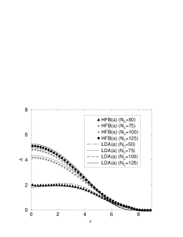
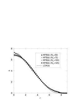
Figure 1: Pairing field $\Delta$ (in units of $\hbar\omega$) as a function of the distance $r$ (in units of $l_{ho}$) from the center of the trap, calculated for the parameters $\mu=32\hbar\omega$ and $g=-1\hbar^{2}l_{ho}/m$, corresponding to $N\approx 1.7\times 10^{4}$ particles in the trap. The different curves have been obtained within the HFB and LDA formalisms using the regularization prescription (a) for different values of the cutoff $N_{C}$.

Figure 2: Same as Fig. 2, but with regularization prescription (b). Remember that with this prescription the LDA result [Eq. (32)] is independent of the cutoff $N_{C}$.

We observe in Fig. 2 that the agreement between LDA and HFB is reasonable for all values of the cutoff $N_{C}$. We also notice that for $N_{C}=125$, which is the maximum value that we considered, the convergence has not yet been reached and therefore the pairing field would grow further if we could increase the cutoff above 125. In Fig. 2 we present the same calculations made with the choice (b) for the regularization. Remember that with this choice, the pairing field within LDA is independent of $N_{C}$ once $N_{C}$ lies above the Fermi surface. On the other hand, the HFB results saturate quite fast and are already very close to convergence for $N_{C}=75$. Again, the LDA and HFB results are in reasonable agreement.

By comparing Figs. 2 and 2 one observes clearly that the calculations (a), Fig. 2, are still quite far from convergence even for the highest considered cutoff. We argue that the convergence rate of method (a), which is the same convergence rate as that of HFB without TFA in the regularization prescription brca , is much slower than that of method (b). This is more evident in Fig. 3 where we plot the HFB values of the pairing field in the center of the trap, $\Delta(0)$, for the two regularization prescriptions (a) (stars) and (b) (diamonds) as a function of the cutoff $N_{C}$. We also plot the results obtained within the LDA(a) (full line) and LDA(b) (dashed line) up to a cutoff of $N_{C}=10^{4}$. In the inset of the figure we magnify the region of cutoff values between 50 and 150. We can observe in the inset that the LDA(a) curve fits well the calculated points for HFB(a). We noticed that the LDA(a) results converge slowly towards a pairing field of about $6.86\hbar\omega$, at a very high cutoff, $N_{C}=10^{6}$. For $N_{C}=10^{3}$ the pairing field in LDA(a) is still only $6.37\hbar\omega$. This very slow convergence rate can be understood within the LDA by taking the ratio of the pairing fields corresponding to the methods (a) and (b). Using Eq. (32) in the limit of very large $k_{C}$, one can derive the relation

$$\frac{\Delta_{\mathit{LDA(a)}}(\bm{r})}{\Delta_{\mathit{LDA(b)}}(\bm{r})}\approx 1-\frac{|g|\sqrt{2}\,[\mu-W(\bm{r})]}{3\pi^{2}\sqrt{N_{C}}}+\cdots\,,$$ (33)

where $W(\bm{r})$ represents the Hartree field (in the present case, $W(0)\approx-16\hbar\omega$).

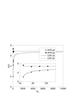
Figure 3: Value of the pairing field in the center of the trap, $\Delta(0)$ (in units of $\hbar\omega$), as a function of the cutoff $N_{C}$, obtained from HFB calculations with the regularization methods (a) (stars) and (b) (diamonds), and from the LDA, method (a) (solid line) and method (b) (dashed line). The parameters $\mu$ and $g$ are the same as in Fig. 2.

As the agreement between LDA(a) and HFB(a) is good in the region up to $N_{C}=125$, we suppose that the convergence rate for HFB(a) is the same as for LDA(a). On the contrary, within HFB(b) the values of the pairing field in the center of the trap are $6.81\hbar\omega$ for $N_{C}=100$ and $6.86\hbar\omega$ for $N_{C}=125$: we conclude that the convergence in this case is much faster. In what follows we will always use the method (b) for the regularization procedure.

III.2 Validity of the LDA at zero temperature

As mentioned before, the parameters used for the calculations shown in Figs. 2, 2, and 3 correspond to a trap with about $1.7\times 10^{4}$ atoms. In this case we found a good agreement between the numerical HFB results and the results obtained from the LDA. However, one might wonder under which conditions the LDA is valid. To study this question, one has to look at systems containing smaller numbers of particles, since in smaller systems the quantum effects (in particular shell effects) which are neglected in the LDA, are supposed to be more important.

In Fig. 4 we present the HFB (full line) and LDA (dashed line) results for the pairing field in the center of the trap, $\Delta(0)$, as a function of the number of atoms $N$. The calculations are done again at zero temperature and with a coupling constant $g=-1$ in trap units. We observe that the two calculations are in reasonable agreement for numbers of atoms greater than about $5000$, which confirms the expectation that the LDA is a valid approximation for systems with a large number of atoms.

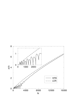
Figure 4: Value of the pairing field in the center of the trap, $\Delta(0)$ (in units of $\hbar\omega$), as a function of the number of particles, $N$, obtained from HFB (solid line) and LDA (dashed line) calculations [regularization method (b), cutoff $N_{C}=100$, coupling constant $g=-1$ in trap units].

What is particularly interesting to look at in this figure is the region $N\lesssim 3000$. In this region the HFB results clearly show the shell structure: the pairing field becomes zero for $N=240,330,440,\dots$, which are the harmonic oscillator “magic numbers”. One also realizes that the central value of the pairing field is smaller if the outer shell corresponds to odd-parity states, than in the case where the outer shell corresponds to even-parity states. This can be understood easily, since the main contribution to the pairing field comes from the states near the Fermi surface, and only $s$ states can contribute to the pairing field at $r=0$. Usually one expects that the LDA should at least reproduce the value of the pairing field if the fluctuations due to shell effects are averaged out, but our results show that the pairing field calculated within the LDA is systematically too high. This might be related to the fact that we are looking at the pairing field at one particular point ($\bm{r}=0$) rather than at the average gap at the Fermi surface, as proposed in LABEL:Farine.

When the number of atoms grows, above a value of about $2500$ the shell structure starts to be washed out and gradually disappears due to the stronger and stronger pairing correlations. This happens in the region where the pairing field grows up to a value of about $\hbar\omega$: when the pairing field becomes comparable with the oscillator level spacing the pairing correlations in a closed shell system can diffuse pairs of atoms towards the higher energy empty shell, resulting in a non-zero pairing field. Globally, we observe that for $N>5000$ the agreement between HFB and LDA is acceptable, even if the LDA systematically overestimates the value of the pairing field at the center.

Of course, the number of particles needed for the validity of the LDA depends on the strength of the interaction; the true criterion which has to be fulfilled reads $\Delta_{\mathit{LDA}}>\hbar\omega$. This criterion can even be applied locally, as one can see in Fig. 2: there the HFB and LDA results are in perfect agreement except in the region of $r\gtrsim 5.5l_{ho}$, where $\Delta$ becomes smaller than $\hbar\omega$.

III.3 Results for non-zero temperature

Now we will discuss some results for temperatures different from zero. We are particularly interested in the following question: Within the LDA, the critical temperature $T_{C}$ is different at each point $\bm{r}$, i.e., when the temperature increases, the order parameter vanishes at last in the center of the trap, where the local critical temperature is the highest. In contrast to this, within the HFB theory, the gap and the critical temperature are global properties, and naively one would expect that, as long as the temperature is below $T_{C}$, the pairing field extends over the whole volume of the system. We will see that even in cases where the LDA works well at zero temperature, it fails at non-zero temperature. On the other hand, also the notion that the gap vanishes globally at $T=T_{C}$, has to be revised in these cases.

In Figs. 6 and 6 we show the HFB and LDA pairing fields obtained at different temperatures, again for $g=-1$ (in trap units) and regularization method (b). The chemical potentials chosen are $\mu=32\hbar\omega$ in Fig. 6 and $\mu=40\hbar\omega$ in Fig. 6, corresponding to approximately $1.7\times 10^{4}$ and $4\times 10^{4}$ particles, respectively. We observe that the good agreement obtained at zero temperature is deteriorated at higher temperatures. In Fig. 6, already at $T=2\hbar\omega/k_{B}$ the LDA reproduces badly not only the tail of the pairing field profile, but also the pairing field in the central region of the trap, in spite of the fact that the pairing field is still large compared with $\hbar\omega$ at this temperature. The LDA description gets worse and worse for higher temperatures and results in an overestimation of the central pairing field and in a too drastic cut of the queue of the profile at large distances. Finally, the LDA method predicts a higher critical temperature than the HFB one. We observed that $T_{C}$ is equal to $3.89$ (in units of $\hbar\omega/k_{B}$) for LDA and to $2.98$ for HFB. In Fig. 6, the agreement is somewhat better. Since the critical temperature is higher than in the previous case, the agreement between LDA and HFB is maintained in a wider range of temperatures. Up to $T=4$ one can see that at least the central region of the trap is well described by LDA. For higher temperatures, we observe the same kind of deterioration of the LDA results shown in Fig. 6. Again, the critical temperature is higher in LDA ($7.08$) than in HFB ($5.97$).

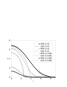
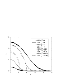
Figure 5: Pairing field $\Delta$ (in units of $\hbar\omega$) as a function of the distance $r$ (in units of $l_{ho}$) from the center of the trap, for a chemical potential $\mu=32\hbar\omega$, corresponding to about $1.7\times 10^{4}$ atoms in the trap [regularization method (b), cutoff $N_{C}=100$, coupling constant $g=-1$ in trap units]. Results obtained within numerical HFB calculations (symbols) are compared with LDA results (lines) for different temperatures $T$.

Figure 6: Same as Fig. 6, but for a chemical potential of $\mu=40\hbar\omega$, corresponding to $N\approx 4\times 10^{4}$ atoms in the trap.

It is evident that the LDA does not correctly describe the phase transition in both cases. On the other hand, also within the HFB calculations one finds that with increasing temperature the pairing field becomes more and more concentrated in the center of the trap. Such a behavior has been predicted in LABEL:BaranovPetrov using the GL theory, the only assumption being that the critical temperature is large compared with the trapping frequency, $k_{B}T_{C}\gg\hbar\omega$. Let us briefly review the main results from this theory and compare them with the results obtained from our HFB calculations (the corresponding numbers are listed in Table 1).

$\mu$	$k_{F}(0)|a|$	$T_{C}^{(0)}$	$T_{C}$	$\delta T_{C}$	$\delta T_{C}^{(GL)}$	$l_{\Delta}$	$l_{\Delta}^{(GL)}$
32	0.78	3.89	2.98	0.91	1.12	1.44	1.23
40	0.91	7.08	5.97	1.11	1.29	1.28	0.95

Table 1: Comparison of results (in trap units) obtained from HFB calculations for the two cases $\mu=32$ and $\mu=40$ shown in Figs. 6 and 6 [coupling constant $g=1$ in trap units, regularization method (b), $N_{C}=100$] and the corresponding results obtained from the GL theory.

In the GL theory the critical temperature $T_{C}$ is predicted to be lower than the critical temperature $T_{C}^{(0)}$ obtained from the LDA. The difference can be written as

$$\delta T_{C}= T_{C}^{(0)}-T_{C}$$

$$= \frac{3\hbar\Omega}{k_{B}}\sqrt{\frac{7\zeta(3)}{48\pi^{2}}\Big{(}1+\frac{\pi}{4k_{F}(0)|a|}\Big{)}}\,,$$ (34)

where $\zeta$ denotes the Riemann zeta function ($\zeta(3)=1.202\dots$). In the derivation of Eq. (34) in LABEL:BaranovPetrov the Hartree potential has been neglected. Here we will include the Hartree potential by using an effective oscillator frequency $\Omega>\omega$. Since near $T_{C}$ the pairing field is concentrated in the center of the trap, we define $\Omega$ by expanding the potential around $r=0$:

$$\Omega=m\sqrt{\bm{\nabla}^{2}[U_{0}(\bm{r})+W(\bm{r})\big{)}]_{\bm{r}=0}}\,.$$ (35)

Within the Thomas-Fermi approximation for the density profile the effective oscillator frequency can be written as

$$\Omega=\frac{\omega}{1-\frac{2k_{F}(0)|a|}{\pi}}\,.$$ (36)

The estimates for $\delta T_{C}$ obtained by inserting the numerical values for $k_{F}(0)|a|$ given in Table 1 into Eqs. (34) and (36) are very reasonable. This can be seen by comparing them with the $\delta T_{C}$ values obtained from the HFB calculations, which are also listed in Table 1. If one considers that these numbers can only be a rough estimate, since $k_{B}T_{C}$ is not really very large compared with $\hbar\Omega$, the agreement with the HFB results is very satisfying.

Not only the critical temperature, also the shape of the order parameter near the critical temperature can be obtained from the GL theory. It can be shown that for temperatures very close to $T_{C}$ the pairing field has the form of a Gaussian,

$$\Delta(\bm{r})=\Delta(0)\exp\Big{(}-\frac{\bm{r}^{2}}{2l_{\Delta}^{2}}\Big{)}\,.$$ (37)

In contrast to the LDA result, the radius $l_{\Delta}$ of this Gaussian is predicted to stay finite in the limit $T\to T_{C}$, as it is the case for the solution of the HFB equations. Its value is given by

$$l_{\Delta}^{2}=R_{TF}^{2}\frac{\hbar\Omega}{k_{B}T}\sqrt{\frac{7\zeta(3)}{48\pi^{2}}\,\frac{1}{1+\frac{\pi}{4k_{F}(0)|a|}}}\,.$$ (38)

In LABEL:BaranovPetrov the quantity $R_{TF}$ was defined as the Thomas-Fermi radius of the cloud, $R_{TF}=\sqrt{2\mu/(m\omega^{2})}$. Generalizing the derivation of Eq. (38) to the case of a non-vanishing Hartree field, we see that the corresponding parameter for the pairing field near the center of the trap is given by

$$R_{TF}\to\, \sqrt{\frac{2[\mu-W(0)]}{m\Omega^{2}}}$$

$$=\Big{(}1-\frac{2k_{F}(0)|a|}{\pi}\Big{)}k_{F}(0)l_{ho}^{2}\,.$$ (39)

On the other hand, the HFB pairing fields corresponding to the temperatures next to $T_{C}$ shown in Figs. 6 and 6 are also perfectly fitted by Gaussians. As shown in Table 1, the agreement between the radii obtained from this fit are again in reasonable agreement with the radii obtained from Eqs. (38) and (39). The deviations are of the order of $30\%$, which is even better than one could have expected, since the parameter $\hbar\Omega/(k_{B}T_{C})$ is not very small in the present case.

Finally, let us look more closely at the critical behavior near $T_{C}$. Again, from the GL theory one can derive that for $T\to T_{C}$ the value of the pairing field in the center should go to zero like

$$\Delta(0)=\sqrt{\frac{16\pi^{2}\sqrt{2}}{7\zeta(3)}\,T_{C}(T_{C}-T)}\,.$$ (40)

As shown in Figs. 7 and 8, this formula is very well satisfied by the HFB results in both cases, $\mu=32$ and $\mu=40$ (in trap units). Note that the prefactor in Eq. (40) differs from the prefactor in LDA. In LDA one finds for $T\approx T_{C}^{(0)}$

$$\Delta_{\mathit{LDA}}(0)=\sqrt{\frac{8\pi^{2}}{7\zeta(3)}\,T_{C}^{(0)}(T_{C}^{(0)}-T)}\,.$$ (41)

The different prefactor, as well as the different critical temperature and the finite radius of the pairing field, are due to the “kinetic” term $\propto\Delta\bm{\nabla}^{2}\Delta$ in the GL energy functional, which is absent in the LDA and which is very important for the description of the strongly $\bm{r}$ dependent pairing field near the critical temperature.

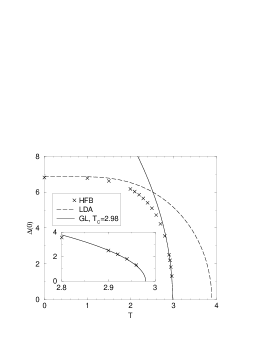
Figure 7: Value of the pairing field in the center of the trap, $\Delta(0)$ (in units of $\hbar\omega$), as a function of temperature $T$ (in units of $\hbar\omega/k_{B}$) for a chemical potential $\mu=32\hbar\omega$, corresponding to about $1.7\times 10^{4}$ atoms in the trap [regularization method (b), cutoff $N_{C}=100$, coupling constant $g=-1$ in trap units]. Results obtained within numerical HFB calculations (symbols) are compared with the LDA result (dashed line) and with the formula (40) obtained from the GL theory (solid line).

Figure 8: Same as Fig. 7, but for a chemical potential of $\mu=40\hbar\omega$, corresponding to $N\approx 4\times 10^{4}$ atoms in the trap.

As a final remark let us mention that the different calculations which we have compared in this paper, are all based on mean-field theory, and therefore do not take into account fluctuations of the order parameter $\Delta$. It is well-known that fluctuations are very important near the phase transition, and in particular in a situation where $k_{F}|a|$ is not small, as it is the case here, they can lead to a considerable change of the critical temperature. Anyway, what we wanted to point out here, is that the LDA gives the wrong $T_{C}$ as compared with a theory taking into account the inhomogeneity of the system. From this result we conclude that in order to have a reliable prediction of $T_{C}$ for the trapped system, it is not sufficient to do a reliable calculation of $T_{C}$ (even including fluctuations) for a homogeneous gas and then apply the LDA.

IV Conclusions

In this paper we have shown a detailed comparison between HFB and LDA calculations at $T=0$ and at $T\neq 0$ for a low density gas of superfluid fermionic atoms trapped by a spherical harmonic potential. We have used a zero-range interaction for the atoms and we have proposed an improvement of the regularization method adopted to remove the ultraviolet divergence brca . This improvement is a modification of a procedure proposed for nuclear systems in LABEL:bul, where the Thomas-Fermi approximation is used in the calculation of the regular part of the Green’s function $G^{0\,\mathit{reg}}_{\mu}$, Eq. (16). The use of the Thomas-Fermi approximation allows to treat systems with a large number of atoms much easier than in the calculations of LABEL:brca. On the other hand, our modification considerably improves the convergence rate of the procedure with respect to the numerical cutoff. By using this regularization method we have observed that the LDA results are in quite good agreement with the corresponding HFB results at zero temperature and for systems with a relatively large number of atoms, where the shell structure effects are washed out. The shell effects, which are important for small systems where the pairing field is smaller than the harmonic level spacing $\hbar\omega$, cannot obviously be reproduced by a LDA calculation.

For non-zero temperatures the agreement between HFB and LDA is deteriorated even in those cases where it was good at $T=0$. In general, LDA overestimates the value of the pairing field in the center of the trap, cuts too drastically the tail of the radial profile of the pairing field at large distances, and overestimates the critical temperature with respect to HFB. We have verified that this discrepancy between the HFB and LDA results at $T$ different from zero can be nicely predicted by using the GL theory BaranovPetrov in cases where the critical temperature is much larger than the harmonic level spacing.

In this article we considered only spherical traps. However, the traps used in experiments are usually cigar-shaped with a low longitudinal and a high transverse trapping frequency, $\omega_{z}\ll\omega_{\perp}$. In this case it is possible that the pairing field, even if it is larger than $\hbar\omega_{z}$, is still smaller than $\hbar\omega_{\perp}$, and the LDA would probably not work. Therefore in principle one should also perform deformed HFB calculations, but at the moment this seems to be numerically very difficult. On the other hand, as noted above, even in the case where $\Delta$ is large compared with both trapping frequencies, the LDA is not adequate at non-zero temperature. Therefore a first step to study non-spherical traps could be to generalize the GL theory of LABEL:BaranovPetrov to the deformed case.

- (1) J.L. Roberts, et al., Phys. Rev. Lett. 86, 4211 (2001).
- (2) B. De Marco and D.S. Jin, Science 285, 1703 (1999); B. De Marco, S.B. Papp, and D.S. Jin, Phys. Rev. Lett. 86, 5409 (2001).
- (3) A.G. Truscott, et al., Science 291, 2570 (2001).
- (4) F. Schreck, G. Ferrari, K.L. Corwin, J. Cubizolles, L. Khaykovich, M.-O. Mewes, and C. Salomon, Phys. Rev. A 64, 011402(R).
- (5) K.M. O’Hara, S.L. Hemmer, M.E. Gehm, S.R. Granade, and J.E. Thomas, Science 298, 2179 (2002).
- (6) M. Houbiers, R. Ferwerda, H.T.C. Stoof, W.I. McAlexander, C.A. Sackett, and R.G. Hulet, Phys. Rev. A 56, 4864 (1997).
- (7) M. A. Baranov and D. S. Petrov, Phys. Rev. A 58, R801 (1998).
- (8) G. Bruun, Y. Castin, R. Dum, and K. Burnett, Eur. Phys. J. D 7, 433 (1999).
- (9) G.M. Bruun and H. Heiselberg, Phys. Rev. A 65, 053407 (2002).
- (10) G.M. Bruun, Phys. Rev. A 66, 041602(R) (2002).
- (11) A. Bulgac and Y. Yu, Phys. Rev. Lett. 88, 042504 (2002).
- (12) N. Nygaard, G.M. Bruun, C.W. Clark, and D.L. Feder, Phys. Rev. Lett. 90, 210402 (2003).
- (13) H. Heiselberg, Phys. Rev. A 63, 043606 (2001).
- (14) E. Timmermans, K. Furuya, P.W. Milonni, and A.K. Kerman, Phys. Lett. A 285, 228 (2001).
- (15) P. Ring and P. Schuck, The Nuclear Many-Body Problem (Springer-Verlag, Berlin, 1980).
- (16) P.-G. de Gennes, Superconductivity of Metals and Alloys (Benjamin, New York, 1966).
- (17) K. Huang, Statistical Mechanics (Wiley, New York, 1987).
- (18) C.A.R. Sá de Melo, M. Randeria, and J.R. Engelbrecht, Phys. Rev. Lett. 71, (1993) 3202.
- (19) E.M. Lifshitz and L.P. Pitaevskii, Statistical Physics, Part 2: Theory of the Condensed State (Pergamon, Oxford, 1980).
- (20) E.R.I. Abraham, W.I. McAlexander, J.M. Gerton, R.G. Hulet, R. Côté, and A. Dalgarno, Phys. Rev. A 55, R3299 (1997).
- (21) M. Farine, F.W.I. Hekking, P. Schuck, and X. Viñas, cond-mat/0207297 (2003).