Macroturbulent Instability of the Flux Line Lattice in Anisotropic Superconductors

Abstract

A theory of the macroturbulent instability in the system containing vortices of opposite directions (vortices and antivortices) in hard superconductors is proposed. The origin of the instability is connected with the anisotropy of the current capability in the sample plane. The anisotropy results in the appearance of tangential discontinuity of the hydrodynamic velocity of vortex and antivortex motion near the front of magnetization reversal. As is known from the classical hydrodynamics of viscous fluids, this leads to the turbulization of flow. The examination is performed on the basis of the anisotropic power-law current-voltage characteristics. The dispersion equation for the dependence of the instability increment on the wave number of perturbation is obtained, solved, and analyzed analytically and numerically. It is shown that the instability can be observed even at relatively weak anisotropy.

74.25.Ha, 74.60.Ge, 74.60.Jg

I Introduction

Magnetic flux dynamics in type-II superconductors has been extensively studied since the end of the 50-s, starting with the pioneering work by A. A. Abrikosov. Primary attention was given to hard superconductors, whose magnetic characteristics are defined by the presence of vortex pinning centers. The main features characterizing the nonuniform penetration of magnetic flux into such systems were revealed and studied; various theoretical models of electrodynamic processes in superconductors were suggested. An avalanche of new researches in this field was triggered by the discovery of high-$T_{c}$ superconductivity (HTS), which brought into play thermal fluctuations and the strong anisotropy of superconductors. Different types of the phase transitions (melting, glass state transitions, etc. ) in the flux line lattice (FLL) have been discovered, studied, and explained. Many of the newly obtained results are described in comprehensive review papers blat ; 2 .

The use of high-resolution magneto-optical (MO) technique enabled an in-depth study of the dynamics of magnetic flux in superconductors. One of the most important features revealed by means of this method is the fractal structures of thermally activated flow of the magnetic flux. Such fractal structures arise usually due to the development of the characteristic instabilities such as macroturbulence in 1-2-3 systems vl ; ind ; joh and dendrite instability in magnesium deboride dendrite . However, these dynamic instabilities in FLL have not been so far properly investigated.

Perhaps, the macroturbulence is the most dramatic phenomena observed in the dynamics of the magnetic flux in HTS. It appears like a turbulization of the FLL motion in a sample near the front of magnetization reversal that separates regions of the vortices of opposite directions (vortices and antivortices). Note that the macroturbulence was only revealed in single-crystal samples of the 1–2–3 system. Its essence is as follows. When a magnetic flux is trapped in a superconductor and a moderate field of a reverse direction is subsequently applied, a boundary of zero flux density will separate the regions containing vortices and antivortices. For definiteness, we apply the term “antivortices” to the vortices whose direction coincides with that of the external magnetic field, and the term “vortices”, to the vortices which were originally present in the sample, prior to switching on the magnetic field of negative sign. At some range of magnetic fields and temperatures, this flux-antiflux distribution becomes unstable. A disordered motion of magnetic flux arises at the front of magnetization reversal, which resembles a turbulent fluid flow. This process rapidly develops in time and is accompanied by the emergence of channels via which the antivortices penetrate into the region occupied by the vortices. In other words, the front of magnetization reversal takes on a finger-like shape. The annihilation of vortices and antivortices occurs at the front, and the process of macroturbulence is soon terminated after a complete disappearance of the vortices. This pattern of penetration of the magnetic flux differs qualitatively from the steady-state slow motion of the front of magnetization upon initial switching on of the magnetic field, when vortices of only one direction are present in the sample. Note that the characteristic times of instability development amount to several seconds and more, and emerging spatial structures are macroscopic, i. e., they contain a large number of single vortices.

The described instability cannot be understood within the framework of the critical state model or conventional models for the thermoactivated flux relaxation. At the same time, this phenomenon is a close analogue to the turbulence in the usual hydrodynamics. So, the study of the phenomenon is of general physical interest. Moreover, this investigation has evident application aspects, since the macroturbulence can affect the ac losses, magnetic noise, and relaxation phenomena in superconducting devices.

An attempt to explain this remarkable behavior of the flux-antiflux interface was undertaken in paper by Bass et al.  bass , where the instability was attributed to a thermal wave generated by the heat release due to the vortex-antivortex annihilation. Unfortunately, this mechanism can hardly be relevant. Indeed, the annihilation energy is small and a corresponding temperature rise is negligible prl ; jetp .

Another physical pattern for the emergence of macroturbulence was discussed by Vlasko-Vlasov et al. hole . They draw attention to the fact that the process of annihilation of a vortex-antivortex pair may be accompanied by the formation of spatial domains free of vortices (the so-called Meissner holes). It was assumed that the presence of such domains may cause instability due to high currents which have to flow in the vicinity of such a Meissner hole. Yet, the authors of Ref. hole, did not describe the possible physical instability mechanism.

An explanation of the macroturbulence should focus on the experimental fact that the instability was reported for $\mathrm{YBa_{2}Cu_{3}O_{7-\delta}}$ and other 1–2–3 single crystals only, which are characterized by the anisotropy in the basal ab plane. This anisotropy can be related to a specific crystallographic structure of these HTS and, in particular, to twin boundaries TB . The electromagnetic instabilities of the critical and resistive states in anisotropic superconductors were considered by Gurevich G1 ; G2 . However, these results cannot be directly applied to the explanation of the turbulent instability.

An alternative approach to understanding the mechanism of the macroturbulence was elaborated in Refs. prl, ; jetp, taking into account of the specific features of the flux motion in the anisotropic superconductors. The anisotropy gives rise to the motion of the flux lines at some angle with respect to the Lorentz force direction. For example, in the presence of twin boundaries, vortices and antivortices move preferably along these guiding boundaries (the so-called guiding effect guid1 ; guid2 ). In general, the angle between the twins and the crystal grains is around $45^{\circ}$. As a result, the flux lines move at some angle with respect to the magnetization reversal front. In our opinion, it is just this circumstance that is of paramount importance to ascertain the nature of macroturbulence. The vortices and antivortices are forced to move towards each other in such a way that the tangential component of their velocity becomes discontinuous at the flux-antiflux interface. According to a classical paper of Helmholtz, a stationary hydrodynamical flow can be unstable and turbulent under such conditions. It was shown prl that a purely hydrodynamic approach which takes into account the anisotropic viscosity of the flux flow can provide the basis to gain an appropriate insight into the nature of the macroturbulence. In particular, the macroturbulence is usually observed within a rather narrow temperature window in the vicinity of 40–50 K bazil . As was demonstrated in Ref. prl, , the temperature window is considerably wider for heavily twinned samples in which a more pronounced anisotropy can be expected.

The model developed in Refs. prl, ; jetp, is based on the analysis of the viscous magnetic flux flow in anisotropic superconductors. In the framework of this model the dependence of the viscosity coefficient of the flux line lattice on the flux velocity was neglected. This approximation corresponds evidently to the description of the superconductor in terms of the linear current-voltage ($I-V$) characteristics. This idealized model allows one to describe qualitatively the effect in question. However, it predicts that the macroturbulence is observable for unrealistically high values of the anisotropy parameter. Note that the regime of the viscous magnetic flux flow is realized at extremely high current densities that cannot be achieved under experimental conditions used in the MO measurement. This is a reason for using a more general model for the flux flow in the present paper. Specifically, we take into account the dependence of the viscosity coefficient on the flux flow rate. In other words, we describe the electric properties of a superconductor by a more realistic non-linear $I-V$ characteristics. We have theoretically studied the instability of the magnetization reversal front under the assumption that the current-voltage characteristic is a power-law function with an exponent $m\geq 1$. We show that, even at a comparatively weak anisotropy of the current-voltage characteristics, the flow of a system of vortices and antivortices in a superconductor can be unstable. A preliminary results of the present study was published in the letter pisma .

II Main equations

The macroturbulence is usually observed in plate-like single crystals placed in a transverse magnetic field. The MO image provides information about the distribution of the normal component of magnetic induction. The penetration of an electromagnetic field into a superconductor in such a geometry is of interest per se and was studied by numerous researchers (see, for example, Refs. G3 ; brandt ). However, the turbulent behavior of magnetic flux is not a geometric effect. It was observed in thin plates and in single crystals with a low demagnetizing factor as well. Frello et al. joh reported the MO visualization of developed macroturbulence of vortex matter in an Nd-123 crystal $3.1\times 2.5\times 1.3$ mm³ in size. In the magnetic field, this sample was divided into three magnetically unbound regions (each having smaller transverse dimensions) in which the turbulence was developing independently. Moreover, it should also be kept in mind that the instability is often observed under conditions of the full penetration of magnetic flux into the sample when the difference in the distribution of induction in the cases of longitudinal and transverse geometry turns out to be not too significant brandt . Therefore, for a qualitative description we can restrict ourselves by the simplest longitudinal geometry. So, consider an infinite superconducting plate of thickness $2d$ in the external magnetic field ${\vec{H}}$ directed parallel to the sample surface along the $z$-axis. The $x$-axis is perpendicular to the plate and the $x$-axis origin, $x=0$, is placed in the plate center (see Fig. 1).

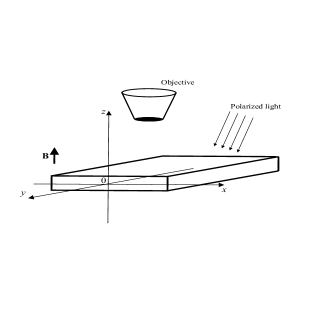
Figure 1: Geometry of the problem.

Let the external magnetic field $H$ first increase up to some value much higher than the lower critical magnetic field $H_{c1}$. Then $H$ is lowered through zero to a negative constant value whose modulus is likewise higher than $H_{c1}$. Under such conditions, two kinds of vortices exist inside the sample. The first one with the magnetic flux directed along the positive $z$-axis has penetrated into the sample under the magnetic field rise (vortices). The vortices occupy the central part of the superconductor. The second group of vortices entering the sample after the external field has changed its sign is characterized by the flux directed oppositely (antivortices). The antivortices are located in two peripheral regions arranged symmetrically relative to the median plane $x=0$ of the plate.

In real crystals, the vortices and antivortices are pinned by defects. The vortex motion occurs due to the action of the Lorentz force and (at non-zero temperature $T$) due to the thermoactivated flux creep. In the framework of the macroscopic description of the flux flow we can take this effect into consideration by making use of the non-linear $I-V$ characteristics blat . There exists an additional reason for the flux line motion in the situation under study. The vortices and antivortices can annihilate near the plane of zero magnetic induction. This phenomenon gives rise to diminishing the vortices number in the bulk and to entering new antivortices through the sample surface. As a result, the line of zero induction moves towards the sample center with time. We will use the phenomenological (hydrodynamic-like) equations to describe the flux line motion. This approach is valid if all spatial scales of the problem are much larger than the FLL constant $d_{f}$. In particular, the characteristic spatial scale of the macroturbulence $l_{c}$ should be large, $l_{c}\gg d_{f}$.

Let us denote the density of the vortices and antivortices as $N_{1}(x,y)$ and $N_{2}(x,y)$, respectively. The relation between vortex densities $N_{\alpha}(x,y)$ and the magnetic induction $B(x,y)$ is evident,

$$N_{\alpha}(x,y)=s_{\alpha}B(x,y)/\Phi_{0},\qquad\alpha=1,2$$ (1)

where $s_{1}=1$, $s_{2}=-1$ and $\Phi_{0}$ is the magnetic flux quantum. ¿From the symmetry of the problem, it is sufficient to consider only the region $0<x<d$. Fig. 2 shows schematically the spatial distributions of $N_{1}(x)$ and $N_{2}(x)$. The vortex and antivortex densities should evidently satisfy the continuity equation,

$$\frac{\partial N_{\alpha}}{\partial t}+\mathrm{div}(N_{\alpha}{\vec{V}}_{\alpha})=0,$$ (2)

where ${\vec{V}}_{\alpha}$ denotes the hydrodynamic velocities of the vortices and antivortices.

In the hydrodynamic approximation, there are two equivalent approaches to find the vortex and antivortex velocities. The usual dynamic approach, where ${\vec{V}}_{\alpha}$ is defined by the viscosity equation for FLL, which takes account of the Lorentz force, was applied in Refs. prl, ; jetp, . The alternative approach implies the use of the $I-V$ characteristics,

$${\vec{J}}={\vec{J}(\vec{E})},$$ (3)

where ${\vec{J}}$ and ${\vec{E}}$ are the macroscopic current density and the electric field. We operate with the latter method in this paper.

Figure 2: Flux distribution in one half of an infinite slab $(|x|\leq d)$ containing trapped vortices of density $N_{1}(x)$ in the central region $|x|\leq x_{0}$, and antivortices of density $N_{2}(x)$ penetrating from the outside. The other symbols are defined in the text.

The velocities and electric field are interrelated by the usual equation,

$${\vec{E}}=\frac{1}{c}{\vec{V}}\times{\vec{B}}.$$ (4)

Using Eq. (1), we can rewrite Eq. (4) in the form,

$$E_{x}=-\frac{N_{\alpha}s_{\alpha}\Phi_{0}}{c}V_{\alpha y},\quad E_{y}=\frac{N_{\alpha}s_{\alpha}\Phi_{0}}{c}V_{\alpha x}.$$ (5)

In principle, we can use the $I-V$ characteristics in general form (3). However, in so doing the obtained results are rather cumbersome and their physical understanding is not evident. To avoid this inconvenience, we use here some particular power-law $I-V$ characteristics for anisotropic superconductors. Let the main anisotropy axes be $X$ and $Y$ (e. g., the $X$-axis is directed along twins, while the $Y$-axis is across them). We suppose that the components of the current density vector along these directions are the odd functions of the electric field and for positive $E$ can be presented as

$$J_{X}=\frac{1}{\varepsilon}J_{c}\left(\frac{E_{X}}{E_{0}}\right)^{1/m},\qquad J_{Y}=J_{c}\left(\frac{E_{Y}}{E_{0}}\right)^{1/m},$$ (6)

where $J_{c}$ is the critical current density along the $Y$ axis, $m>1$ is the corresponding exponent, $\varepsilon<1$ is the anisotropy parameter for the critical current components and the value of $J_{c}$ is defined as the current density $J_{Y}$ at $E=E_{0}$ (usually, $E_{0}$ is accepted as 1 $\mu$V/cm). At $m=1$ the $I-V$ characteristics (6) correspond to the viscous flux flow regime used for the macroturbulence analysis in Ref. prl, . In the limiting case $m\gg 1$, these characteristics are in accordance with the critical state model proposed by Clem clem for the description of the electrodynamics of anisotropic superconductors.

As was mentioned above, the anisotropy in ab plane arises in 1–2–3 single crystals mainly due to the existence of twin boundaries. In a real experimental situation, these boundaries make angles of about $45^{\circ}$ with the axes $x$ and $y$. Therefore, we assume the angle between two coordinate systems, xy and XY, to be equal to $45^{\circ}$. Now, using Eqs. (5), (6) and the Maxwell equation $\nabla\times\vec{B}=4\pi\vec{J}/c$ we can derive the equations interrelating the vortex density and velocity components,

$$\frac{\partial N_{\alpha}}{\partial x}-\frac{\partial N_{\alpha}}{\partial y}=\frac{4\pi\sqrt{2}J_{c}}{c\Phi_{0}\varepsilon}\left[\frac{N_{\alpha}\Phi_{0}}{cE_{0}\sqrt{2}}\left(-V_{x\alpha}+V_{y\alpha}\right)\right]^{{}^{1}/m},$$ (7)

$$\frac{\partial N_{\alpha}}{\partial x}+\frac{\partial N_{\alpha}}{\partial y}=-\frac{4\pi\sqrt{2}J_{c}}{c\Phi_{0}}\left[\frac{N_{\alpha}\Phi_{0}}{cE_{0}\sqrt{2}}\left(V_{x\alpha}+V_{y\alpha}\right)\right]^{{}^{1}/m}.$$

To solve the problem, we must formulate the boundary conditions at the sample surface, as well as at the interface between the domains occupied by the vortices and antivortices. We will first discuss the conditions at the sample boundaries. Ignoring the induction jump on the surface (this may be done in the case of fairly high values of $H$, $H\gg H_{c1}$), one can derive

$$N_{2}(d)=N_{2}(-d)=H/\Phi_{0}.$$ (8)

Since only the right-hand part $0<x<d$ of the sample is treated, we will replace the condition $N_{2}(-d)=H/\Phi_{0}$ by the requirement,

$$V_{\alpha}(0)=0,$$ (9)

that immediately follows from the symmetry of the problem.

Now we turn to the boundary conditions at the moving vortex-antivortex interface. In general case, the position of the interface depends on time $t$ and the $y$ coordinate. The equation for this surface can be presented as $x=x_{0}(y,t)$. Then, one can define the interface velocity $\vec{U}$ as a vector normal to this surface,

$$U_{x}=\frac{\partial x_{0}}{\partial t}\frac{1}{1+(\partial x_{0}/\partial y)^{2}},$$

$$U_{y}=-\frac{\partial x_{0}}{\partial t}\frac{\partial x_{0}/\partial y}{1+(\partial x_{0}/\partial y)^{2}}.$$ (10)

In general, the velocity $\vec{U}$, just as $x_{0}(y,t)$, depends on time and the coordinate $y$, $\vec{U}=\vec{U}(y,t)$.

In the coordinate system which moves with the interface, the total flux of the vortex and antivortex densities through the interface should vanish due to the evident vortex conservation law. This means that the following boundary condition should be fulfilled at $x=x_{0}$,

$$N_{1}\left(\vec{V_{1}}-\vec{U}\right)_{n}+N_{2}\left(\vec{V_{2}}-\vec{U}\right)_{n}=0,$$ (11)

where the subscript $n$ denotes the vector components transverse to the interface. The components of the corresponding normal unit vector $\vec{\nu}$ are

$$\nu_{x}=\frac{1}{\sqrt{1+\left(\partial x_{0}/\partial y\right)^{2}}},$$

$$\nu_{y}=-\frac{\partial x_{0}/\partial y}{\sqrt{1+\left(\partial x_{0}/\partial y\right)^{2}}}.$$ (12)

The second boundary condition should define the rate of the vortex-antivortex annihilation. It is obvious that this rate goes to zero if the density of vortices or antivortices at the interface between them is zero. Then, following the conventional approach to describing such kinetic processes, we represent the rate of annihilation to be proportional to the product of the vortex and antivortex densities,

$$N_{1}({\vec{V}}_{1}-{\vec{U}})_{n}=RN_{1}N_{2}.$$ (13)

A similar model for the annihilation process was used in Ref. bass, . The finite size region where the annihilation occurs was supposed to exist in the sample. The annihilation rate was assumed to be proportional not only to the product $N_{1}$ and $N_{2}$ but also to the relative velocity $|V_{1}-V_{2}|$ of the vortices and antivortices. Contrary to Ref. bass, , we believe that the region where vortices and antivortices coexist and annihilate is small enough and is much less as compared not only to the sample sizes but also to the characteristic spatial scale $l_{c}$ of the macroturbulence. This assumption can be confirmed by MO images of the macroturbulent instability vl ; ind ; joh . It means, in particular, that the annihilation constant $R$ is not too small. Thus, the flux-antiflux boundary can be represented by the surface $x=x_{0}(y,t)$.

Finally, we assume that the average magnetic induction in the neighborhood of the interface is zero, i.e.,

$$N_{1}=N_{2}$$ (14)

at $x=x_{0}(y,t)$. One can readily demonstrate that this condition directly follows from Eq. (2) and relation (11), if it was valid at the moment of emergence of antivortices into the sample. In our case, $N_{1}=N_{2}=0$ at the time moment when the decreasing external magnetic field assumed the value of $H=0$.

III Unperturbed profile of the vortex distribution

The formulated set of equations and boundary conditions allow us, in principle, to analyze the behavior of the vortex-antivortex system. We assume that the unperturbed flux-antiflux boundary is a straight line. A scheme of solving the problem consists in finding the unperturbed vortex distribution $N_{\alpha}(x,t)$ and velocity $V_{\alpha}(x,t)$. Using these base distributions, one should solve a linearized set of equations for fluctuations $\delta N_{\alpha}(x,y,t)$ and $\delta V_{\alpha}(x,y,t)$. This section is devoted to the analysis of the base profile. Below we take into account the dependence of the critical current density $J_{c}$ on the magnetic induction $\Phi_{0}N_{\alpha}$. For definiteness sake, we choose it in the simplest form,

$$J_{c}=A/N_{\alpha}.$$ (15)

To find the base profile of the vortex density it is necessary to solve a complex set of partial differential equations (2)–(7) along with the boundary conditions (8)–(14) some of which are written at the moving interface. A peculiar complication consists in the fact that the velocity $U(t)$ of the motion of the vortex-antivortex interface is unknown and should be found self-consistently. Unfortunately, the problem does not have simple (with $U=\mathrm{const}\neq 0$) automodel solutions because the interface moves non-uniformly under the conditions being studied.

As the first approximation, let us calculate a stationary base profile of another system where the velocity $U(t)$ equals zero. A superconducting slab carrying the critical transport current is an example where such a distribution of the vortices and antivortices can be realized. Assuming $\partial N_{\alpha}/\partial t=0$ in Eq. (2), one can easily obtain the distributions $N_{1}(x)$ and $N_{2}(x)$,

$$\displaystyle N_{\alpha}(x)=N_{0}\sqrt{1+s_{\alpha}C(x_{0}-x)/d},$$ (16)

$$\noindent C=\frac{8\pi\sqrt{2}dA}{c\Phi_{0}N_{0}^{2}}\cdot\left[\frac{\sqrt{2}\Phi_{0}RN_{0}^{2}}{cE_{0}(1+\varepsilon^{m})}\right]^{1/m},$$

from Eqs. (2)–(7) and conditions (11)–(14). Following the experiments vl ; ind ; joh which show that the vortex density $N_{0}$ at the interface is small with respect to its value $N_{2}(d)=H/\Phi_{0}$ at the sample surface, we assume the constant $C$ to be much higher than unity. Neglecting unity in the radicand in Eq. (16) and using condition (8) one can evaluate the vortex density $N_{0}$ at the interface,

$$N_{0}=N_{\alpha}(x=x_{0})\sim\left(\frac{H}{H_{p}}\right)^{m}\left(\frac{cE_{0}}{2^{(m+1)/2}\Phi_{0}R}\right)^{1/2},$$ (17)

$$H_{p}=(8\pi dA\Phi_{0}/c)^{1/2}.$$

Expression (16) is the solution of the stationary problem. We are interested in the base profile corresponding to the moving interface. This motion leads to a distortion of the profile with respect to Eq. (16). However, we assume the velocity $U$ to be small with respect to the vortex velocity $V_{\alpha}$, $U\ll V_{\alpha}$. As it can be readily shown, in this case the base profile differs but slightly from the stationary distribution (16).

It is convenient to perform the further analysis using the dimensionless variables,

$$\displaystyle n_{\alpha}=N_{\alpha}/N_{0},\quad\tau=t/t_{0},\quad t_{0}=\frac{\Phi_{0}^{2}N_{0}^{3}}{8\pi AE_{0}},$$

$$\noindent\ \xi=x/L,\quad\zeta=y/L,\quad L=\frac{c\Phi_{0}N_{0}^{2}}{4\pi\sqrt{2}A},$$

$$\noindent r=\frac{RN_{0}^{2}\Phi_{0}}{\sqrt{2}cE_{0}},\quad u=Ut_{0}/L.$$ (18)

The normalization to the time-dependent value $N_{0}=N_{\alpha}(x_{0}(t))$ is allowable here since we assume that the instability develops much faster than noticeable changes in $N_{\alpha}(x_{0})$ and $U(t)$ occur.

Taking into account the smallness of the velocity $u(\tau)$ of the flux-antiflux boundary, we can linearize the expression for the base profile $n_{\alpha}(\xi,\tau)$ with respect to $u$. In so doing, we get the equations for the first and second derivatives, $n_{\alpha}^{{}^{\prime}}$ and $n_{\alpha}^{{}^{\prime\prime}}$, of the unperturbed vortex density near the interface,

$$\displaystyle n_{\alpha}^{{}^{\prime}}(x=x_{0})=-s_{\alpha}\rho\left(1+s_{\alpha}\frac{u}{rm}\right),$$ (19)

$$\noindent n_{\alpha}^{{}^{\prime\prime}}(x=x_{0})=-(n_{\alpha}^{{}^{\prime}})^{2}-\frac{2u}{(1+\epsilon)m(n_{\alpha}^{{}^{\prime}})^{m-2}},$$ (20)

$$\noindent\epsilon=\varepsilon^{m},\quad\rho=\left(\frac{2r}{1+\epsilon}\right)^{1/m}.$$

These formula are used in the next section devoted to the analysis of the instability.

IV Instability in the vortex-antivortex system

Let the dimensionless vortex density be a sum of the unperturbed term $\tilde{n}_{\alpha}(\xi,\tau)$ and a fluctuation term,

$$n_{\alpha}=\tilde{n}_{\alpha}+f_{\alpha}(\xi-\xi_{0}(\tau))\exp(\lambda\tau+{\rm i}k\zeta).$$ (21)

The linearized boundary conditions should be written at the perturbed interface,

$$\xi=\xi_{0}(\zeta,\tau)=\xi_{0}(\tau)+\delta\xi\exp({\rm i}k\zeta+\lambda\tau).$$ (22)

It follows directly from Eq. (11) that

$$\delta\xi=(f_{1}-f_{2})/2\rho.$$ (23)

Substituting Eq. (21) into Eq. (2) and neglecting the terms proportional to $\epsilon^{2}$, we derive the ordinary differential equation with the coordinate-dependent coefficients for the fluctuation $f_{\alpha}(\xi-\xi_{0}(\tau))$,

$$f_{\alpha}^{{}^{\prime\prime}}+2f_{\alpha}^{{}^{\prime}}\left[\mathrm{i}k(1-2\epsilon)+\frac{\tilde{n}_{\alpha}^{{}^{\prime}}}{\tilde{n}_{\alpha}}-u\frac{m-2}{m{\tilde{n}_{\alpha}^{{}^{\prime}(m-1)}}{\tilde{n}_{\alpha}^{m}}}\right]-$$

$$\frac{2\lambda}{m{\tilde{n}_{\alpha}^{{}^{\prime}(m-1)}}{\tilde{n}_{\alpha}^{m}}}-\frac{2u}{{\tilde{n}_{\alpha}^{{}^{\prime}(m-2)}}{\tilde{n}_{\alpha}^{(m+1)}}}-\frac{2u\mathrm{i}k(m-1)}{m{\tilde{n}_{\alpha}^{{}^{\prime}(m-1)}}{\tilde{n}_{\alpha}^{m}}}-$$

$$\frac{{\tilde{n}_{\alpha}^{{}^{\prime}2}}}{{\tilde{n}_{\alpha}^{2}}}-k^{2}+2\mathrm{i}k\frac{\tilde{n}_{\alpha}^{{}^{\prime}}}{{\tilde{n}_{\alpha}}}=0.$$ (24)

We assume the perturbation of the vortex density to be damped away from the interface $\xi=\xi_{0}(\tau)$ at short distances with respect to the sample thickness $d$. This allows us to replace the coordinate-dependent variables ${\tilde{n}_{\alpha}}(\xi)$ and ${\tilde{n}_{\alpha}}^{{}^{\prime}}(\xi)$ in Eq. (24) by their values ${\tilde{n}_{\alpha}}(\xi=\xi_{0})$ and ${\tilde{n}_{\alpha}}^{{}^{\prime}}(\xi=\xi_{0})$ at the interface (see Eq. (19)).

The solution of Eq. (24) defines the exponential behavior of the fluctuations $f_{1}$ and $f_{2}$,

$$f_{1}(\xi-\xi_{0})=f_{1}\exp[p_{1}(\xi-\xi_{0})],$$

$$f_{2}(\xi-\xi_{0})=f_{2}\exp[p_{2}(\xi-\xi_{0})],$$ (25)

where

$$p_{1,2}=\pm\rho-\mathrm{i}k+\rho u/2r\pm\Omega_{1,2},$$ (26)

$$\Omega_{1,2}=\left[2\rho^{2}+\frac{\mathrm{i}ku\rho}{mr}+\frac{\lambda\rho}{mr}+4\epsilon k^{2}\mp\frac{\mathrm{i}ku\rho(m-1)u}{m^{2}r^{2}}\pm\right.$$

$$\left.\frac{2u\rho^{2}}{mr}\mp\frac{\lambda\rho(m-1)u}{m^{2}r^{2}}\right]^{1/2},\qquad\mathrm{Re}\,\Omega_{1,2}>0.$$ (27)

Here the upper and lower signs correspond to the coefficients $p_{1}$ and $p_{2}$, respectively.

Substituting Eqs. (21)–(27) into the boundary conditions (11), (13) gives two linear algebraic homogeneous equations for $f_{1}$ and $f_{2}$,

$$\displaystyle f_{1}\left[-\frac{m}{2}{\tilde{n}_{1}}^{{}^{\prime}(m-1)}(p_{1}+\mathrm{i}k(1-2\epsilon)+{\tilde{n}_{1}}^{{}^{\prime}})-\frac{\mathrm{i}ku(1-3\epsilon)}{\rho}-u-\frac{\lambda}{\rho}\right]+$$

$$f_{2}\left[-\frac{m}{2}{\tilde{n}_{2}}^{{}^{\prime}(m-1)}(p_{2}+\mathrm{i}k(1-2\epsilon)+{\tilde{n}_{2}}^{{}^{\prime}})+\frac{\mathrm{i}ku(1-3\epsilon)}{\rho}-u+\frac{\lambda}{\rho}\right]=0,$$ (28)

$$\displaystyle f_{1}\left[-\frac{m}{2}{\tilde{n}_{1}}^{{}^{\prime}(m-1)}(p_{1}+\mathrm{i}k(1-2\epsilon)+{\tilde{n}_{1}}^{{}^{\prime}})+\frac{\mathrm{i}k(1-2\epsilon)}{4\rho}{\tilde{n}_{1}}^{{}^{\prime}m}-\frac{\lambda}{2\rho}-r-u\frac{m-1}{m}-\frac{u\epsilon{\tilde{n}_{1}}^{{}^{\prime}}}{2\rho}\right]+$$

$$f_{2}\left[\frac{\lambda}{2\rho}-\frac{\mathrm{i}k(1-2\epsilon)}{4\rho}{\tilde{n}_{1}}^{{}^{\prime}m}-r-\frac{u}{m}+\frac{u\epsilon{\tilde{n}_{1}}^{{}^{\prime}}}{2\rho}\right]=0.$$ (29)

Here we took into account that the normal unit vector to the perturbed interface is ${\vec{\nu}}=(1,\;-{\rm i}k\delta\xi(\zeta,\tau))$.

Requiring that the determinant of set (IV), (IV) should vanish and omitting the terms of the order of $u^{2}\ll 1$, one obtains the dispersion equation for the increment $\lambda$ at different values of the wave number $k$,

$$\lambda=\frac{mr}{\rho}\left(\Omega^{2}-4\epsilon k^{2}-\mathrm{i}ku\frac{\rho}{mr}-2\rho^{2}\right).$$ (30)

Here $\Omega$ is the root with $\mathrm{Re}\,\Omega>0$ of the equation

$$\displaystyle\Omega^{4}+\Omega^{3}\rho\frac{m+2}{m}-2\Omega^{2}\rho^{2}\frac{m-1}{m}-4\Omega\frac{\rho^{3}}{m}-$$

$$\mathrm{i}ku\frac{\rho}{m^{2}r}\left(\Omega^{2}\frac{m-1}{2}+\Omega\frac{\rho m}{2}+\rho^{2}m\right)-$$

$$4\epsilon k^{2}\left(\Omega^{2}+\Omega\frac{2\rho}{m}+\mathrm{i}ku\frac{\rho(m-1)}{2m^{2}r}\right)=0.$$ (31)

Below we perform the analysis of this equation in two qualitatively different limiting cases.

IV.1 Linear viscosity, $m=1$

The vortex motion in the case $m=1$ can be described in terms of the magnetic flux viscose flow with the constant anisotropic viscosity coefficient. Indeed, the current-voltage characteristics (6), (15) leads to the linear tensor relationship between the vortex velocity and the Lorentz driving force,

$$\Gamma_{ik}N_{\alpha}V_{\alpha k}=F_{Li},\qquad{\vec{F}}_{L}=\frac{1}{c}{\vec{B}}\times{\vec{J}},$$ (32)

where the viscosity tensor $\Gamma_{ik}$ is characterized by the principal values

$$\Gamma_{XX}=\frac{\Phi_{0}^{2}}{c^{2}}\frac{A}{E_{0}},\qquad\Gamma_{YY}=\frac{\Phi_{0}^{2}}{c^{2}\varepsilon}\frac{A}{E_{0}}.$$ (33)

At $m=1$, Eq. (IV) takes on the form,

$$\Omega^{4}+6r\Omega^{3}-32r^{3}\Omega-2\mathrm{i}kur(\Omega+4r)-$$

$$4\epsilon k^{2}\Omega(\Omega+4r)=0.$$ (34)

It has a simple solution with the following asymptotics at $k\rightarrow\infty$, $\varepsilon\rightarrow 0$,

$$\Omega\approx(2k|u|r)^{1/3}\exp(-\mathrm{i}\pi/6).$$ (35)

The corresponding increment $\lambda$ increases unrestrictedly at $k\rightarrow\infty$,

$$\lambda\approx(k|u|r/4)^{2/3}-\mathrm{i}ku.$$ (36)

Considering the finite value of $\varepsilon$ limits this increase to a certain maximum value of Re$\lambda_{m}$ prl ,

$$\mathrm{Re}\,\lambda_{m}\approx\frac{|u|r}{8\varepsilon^{1/2}}-4r^{2},\qquad k_{m}\approx\frac{(|u|r)^{1/2}}{(4\varepsilon)^{3/4}}.$$ (37)

The existence of the solution with $\mathrm{Re}\,\lambda>0$ means that the instability of the base profiles near the flux-antiflux interface exists. The increment of the instability grows with an increase of the wave number if $k<k_{m}$. Therefore, the perturbations with the characteristic spatial scale $l_{c}\sim 1/k_{m}$ along the $y$-axis is predominant over others. Thus, the flux-antiflux interface is disturbed in a turbulent-like manner LL and we can suppose that the presented mechanism of the macroturbulence could explain the experiment.

As was shown in Ref. prl, , the instability exists for very small $\varepsilon$ only,

$$\varepsilon\leq 0.019\left[\frac{U}{2RN_{0}}\right]^{2}\ll 1.$$ (38)

So stringent a requirement imposed on the parameter of anisotropy prompted us to consider the more general situation of arbitrary $m$. The case $m\gg 1$ is discussed in the next subsection.

IV.2 Power-law current-voltage characteristics, $m\gg 1$

The parameter $\epsilon=\varepsilon^{m}$ in Eq. (IV) becomes negligible at $m\gg 1$. Therefore, Eq. (IV) transforms into

$$X^{4}+\frac{m+2}{m}X^{3}-2\frac{m-1}{m}X^{2}-\frac{4}{m}X+$$

$${\rm i}\kappa\left(\frac{m-1}{m}X^{2}+X+2\right)=0,$$ (39)

$$X=\frac{\Omega}{\rho},\qquad\kappa=k|u|/2mr\rho.$$

Contrary to Eq. (IV.1), this equation contains the term ${\rm i}\kappa X^{2}(m-1)/m$ which plays an essential role at $\kappa\gg 1$ and changes radically the character of the solution:

$$X\approx\kappa^{1/2}\exp\left(-\frac{{\rm i}\pi}{4}\right)-\frac{1}{2m}-\frac{2}{\kappa^{1/2}}\exp\left(\frac{{\rm i}\pi}{4}\right).$$ (40)

The correspondent increment $\lambda$,

$$\lambda\approx mr\rho\left({\rm i}\kappa+2-\frac{\kappa^{1/2}}{2^{1/2}m}\right),\quad m,\kappa\gg 1,$$ (41)

is almost an imaginary quantity but its relatively small real part is positive at $\kappa<8m^{2}$. This means that the instability develops as an oscillating process with a magnitude increasing in time. The wave number $\kappa$ of the instability is bounded from above due to the finiteness of the parameter $1/m$. Contrary to the case $m=1$, the instability occurs regardless of the strength of the current anisotropy, practically, if the anisotropy parameter $\varepsilon\ll 1$.

V Numerical analysis and discussion

On the basis of the developed theory, let us analyze the instability of the vortex-antivortex system. In general case of arbitrary $\varepsilon$ and $m$ this analysis requires that the dispersion equation (IV) be numerically solved.

The dependence of the increment Re$\lambda$ on the wave number $\kappa$ for $m=20$ and the different values of the anisotropy parameter $\varepsilon$ is shown in Fig. 3. For definiteness, the value of the ratio $(u/r)^{2}$ is taken to be equal to 0.02. Remind that this ratio should be small in accordance with the assumptions made above. The figure shows that the spectrum of perturbations strongly depends on the parameter of anisotropy.

Figure 3: The numerical solution $\mathrm{Re}\lambda(\kappa)$ of the dispersion equation for $m=20$, $(u/r)^{2}=0.02$ at different values of the anisotropy parameters $\varepsilon$: $\varepsilon=0.5$ (curve 1), $\varepsilon=0.45$ (2), $\varepsilon=\varepsilon_{c}=0.43$ (3), $\varepsilon=0.4$ (4), $\varepsilon=0.38$ (5), and $\varepsilon=0.2$ (6).

Instability is observed at $\varepsilon\leq\varepsilon_{c}\approx 0.43$. Indeed, the increment Re$\lambda$ becomes positive at some interval of the wave number $\kappa$ and reaches the maximum value at finite $\kappa$. If the anisotropy parameter is higher than $\varepsilon_{c}$, the increment Re$\lambda$ is negative at any value of $\kappa$. This implies that the vortex-antivortex system is stable with respect to small perturbations if the current anisotropy of a superconductor is not small enough. Of course, the critical value $\varepsilon_{c}$ of the anisotropy parameter depends strongly on the exponent $m$. The graphs in Fig. 4 illustrate the change in the value of $\varepsilon_{c}$ with an increase of $m$. The function $\varepsilon_{c}(m)$ is not very sensitive to the value of the small parameter $u/r$ in our theory. The graph $\varepsilon_{c}(m)$ represents the separatrix dividing the phase space $(m,\varepsilon)$ into two parts corresponding to the stable (left-hand part) and unstable (right-hand part) states of the vortex system.

One of the most important results of this paper consists in the substantial weakening the requirement theoretically imposed on the anisotropy parameter $\varepsilon$ for the observation of the instability in the vortex-antivortex system. The effective parameter of the anisotropy determining the existence of the instability is $\varepsilon^{m}$ in the considered case of the nonlinear current-voltage characteristics. Since the exponent $m$ can reach several tens in real superconductors, the necessary condition for the instability is achieved for not too small values of $\varepsilon$.

Figure 4: The separatrix dividing the stability and instability regions in the phase plane ($\varepsilon,m$). The solid line corresponds to $(u/r)^{2}=0.02$, the dashed line is obtained for $(u/r)^{2}=0.002$.

This circumstance allows one to eliminate a seeming contradiction between our theory and experiments where the macroturbulence was reported to be observed even in detwinned YBCO single crystals. The MO image of the development of the macroturbulence in such a sample is shown in Fig. 5. The twinning structure in this sample is not observed in polarized light whereas the macroturbulence is clearly pronounced. However, a careful scan of the left top image in Fig. 5, where the initial magnetic flux distribution is shown, highlights the presence of some anisotropy of the current-carrying capability in the sample plain. The penetration depth in the horizontal direction is clearly seen to be about 1.2 times higher than in the vertical one. This means that the anisotropy exists and the macroturbulent instability may appear. Such a situation with the detwinned samples is, perhaps, typical for the 1–2–3 single crystals. After the detwinning procedure, some traces of the twin structure remain inside a sample and the anisotropic distribution of the impurities takes place. The existence of the anisotropy of the electrical resistivity in the ab plane of detwinned YBCO single crystals was reported in Ref. kwok, . Irrespective of its nature, the anisotropy in the detwinned samples can cause the observed macroturbulent instability.

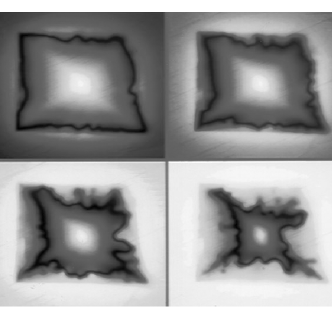
Figure 5: The MO image of the development of the macroturbulence in a detwinned YBCO single crystal.

Finally, we should note that the qualitative features of the studied instability are quite similar at any $m>1$.

VI Conclusion

The very interesting phenomenon of the macroturbulent instability has so far been observed only in superconductors of 1–2–3 systems. Such systems are normally characterized by a well-pronounced anisotropy of the current-carrying capability in the ab plane. This experimental fact provided the basis for the theoretical approach to explain the nature of the instability. Under the action of the Lorentz force, the vortices and antivortices move towards each other at some non-zero angle with respect to the front of magnetization reversal owing to the anisotropy. As a result, the vortex and antivortex hydrodynamic flow is characterized by the tangential discontinuity near the front. Specifically this fact leads to the turbulization. The anisotropy is described in terms of the power-law anisotropic current-voltage characteristics. The analysis of the linearizes set of equations consisting of the continuity and Maxwell equations along with appropriate boundary conditions allowed us to derive the dispersion equation for the increment of the instability. As is shown, the instability exists in a wide range of the parameters of the problem. In particular, the instability can be observed at not very strong anisotropy if the current-voltage characteristics is steep. This conclusion agrees with the experiment.

Unfortunately, we cannot make a direct comparison between the theoretical results and the experimental data because the theory operates with the unknown phenomenological parameter $R$ describing the vortex-antivortex annihilation rate. In order to express this parameter in terms of observable variables, the microscopic model of the annihilation process needs to be constructed. Nevertheless, the proposed theory and the obtained phase diagram, showing the region where the instability occurs, can be useful for the qualitative analysis of the macroturbulence. For instance, the existence of the instability in a definite temperature region alone can be simply rationalized within our model. At low temperatures, the critical current density increases, and the characteristic spatial scale $L$, in Eq. (III), decreases correspondingly and becomes comparable to or less than the twin-boundary spacing. As a result, the anisotropy is suppressed and the instability disappears. On the other hand, at temperatures close to $T_{c}$ the anisotropy is no longer effective due to the thermal activation of the vortices. It is a remarkable thing fully supporting our model, that in the present heavily twinned crystal the turbulence occurs at much lower temperatures than is found in previous studies of similar crystals with only little twinning koblisch ; joh .

- (1) G. Blatter, M. V. Feigel’man, V. B. Geshkenbein, A. I. Larkin, and V. M. Vinokur, Rev. Mod. Phys. 66, 1125 (1994).
- (2) E. H. Brandt, Rep. Prog. Phys. 58, 1465 (1995).
- (3) V. K. Vlasko-Vlasov, V. I. Nikitenko, A. A. Polyanskii, G. W. Grabtree, U. Welp, and B. W. Veal, Physica C 222, 361 (1994).
- (4) M. V. Indenbom, Th. Schuster, M. R. Koblischka, A. Forkl, H. Kronmüller, L. A. Dorosinskii, V. K. Vlasko-Vlasov, A. A. Polyanskii, R. L. Prozorov, and V. I. Nikitenko, Physica C 209, 259 (1993).
- (5) T. Frello, M. Baziljevich, T. H. Johansen, N. H. Andersen, Th. Wolf, and M. R. Koblischka, Phys. Rev. B59, R6639 (1999).
- (6) T. H. Johansen, M. Baziljevich, D. V. Shantsev, P. E. Goa, Y. M. Galperin, W. N. Kang, H. J. Kim, E. M. Choi, M.-S. Kim, S. I. Lee, Appl. Phys. Lett. (2002). ??
- (7) F. Bass, B. Ya. Shapiro, I. Shapiro, and M. Shvartser, Phys. Rev. B58, 2878 (1998).
- (8) L. M. Fisher, P. E. Goa, M. Baziljevich, T. H. Johansen, A. L. Rakhmanov, and V. A. Yampol’skii, Phys. Rev. Lett. 87, 247005-1 (2001).
- (9) A. L. Rakhmanov, L. M. Fisher, V. A. Yampol’skii, M. Baziljevich, and T. H. Johansen, ZhETF 122, 886 (2002) [JETP 95, 768 (2002)].
- (10) V. K. Vlasko-Vlasov, U. Welp, G. W. Crabtree, D. Gunter, V. Kabanov, V. I. Nikitenko, Phys. Rev. B56, 5622 (1997).
- (11) I. F. Voloshin, A. V. Kalinov, L. M. Fisher, K. I. Kugel’, and A. L. Rakhmanov, ZhETF 111, 2158 (1997) [JETP 84, 1177 (1997)].
- (12) A. Gurevich, Phys. Rev. Lett. 65, 3197, (1990).
- (13) A. Gurevich, Phys. Rev. B46, 3638 (1992).
- (14) A. K. Niessen, C. H. Weijsenfeld, J. Appl. Phys., 40, 384 (1969).
- (15) H. Pastoriza, S. Candia, G. Nieva, Phys. Rev. Lett. , 83, 1026 (1999).
- (16) T. Frello, M. Baziljevich, T. H. Johansen, N. H. Andersen,T. Wolf, M. R. Koblischka Phys. Rev. B59, R6639 (1999).
- (17) A. L. Rakhmanov, L. M. Fisher, A. A. Levchenko, V. A. Yampol’skii, M. Baziljevich, and T. H. Johansen, Pis’ma v ZhETF 76, 349 (2002) [JETP Lett. 76, 291 (2002)].
- (18) A. V. Gurevich, Int. J. Mod. Phys. B, 9, 1045 (1995).
- (19) E. H. Brandt, Phys. Rev. Lett. 76, 4030 (1996).
- (20) J. R. Clem, Phys. Lett. 54A, 452 (1975), ibid, Phys. Lett. 59A, 401 (1976).
- (21) L. D. Landau and E. M. Lifshits, Fluid Mechanics (Butterworth-Heinemann, Oxford, 1987).
- (22) U. Welp, S. Fleshler, W. K. Kwok, J. Downey, Y. Fang, G. W. Crabtree, and J. Z. Liu, Phys. Rev. B42, 10189 (1990).
- (23) M. R. Koblischka, T. H. Johansen, M. Baziljevich, H. Hauglin, H. Bratsberg, B. Ya. Shapiro, Europhys. Lett. 41, 419 (1998).