A layered neural network with three-state neurons optimizing the mutual information

Abstract

The time evolution of an exactly solvable layered feedforward neural network with three-state neurons and optimizing the mutual information is studied for arbitrary synaptic noise (temperature). Detailed stationary temperature-capacity and capacity-activity phase diagrams are obtained. The model exhibits pattern retrieval, pattern-fluctuation retrieval and spin-glass phases. It is found that there is an improved performance in the form of both a larger critical capacity and information content compared with three-state Ising-type layered network models. Flow diagrams reveal that saddle-point solutions associated with fluctuation overlaps slow down considerably the flow of the network states towards the stable fixed-points.

1 Introduction

By now it is common knowledge that layered feedforward models are the workhorses in practical applications of neural networks and, hence, progress in the theoretical understanding of their capabilities and limitations should thus be welcome. Recently, it has been shown [1, 2] how information theory can be used to construct neural network models leading to optimal performance. Optimal for the task of retrieving an embedded pattern when the network starts far from it with a vanishingly small initial mutual information. For two-state networks this approach recovers the well-known Hopfield model [3] and for three-state networks a Hamiltonian is found reminiscent of the Blume-Emery-Griffiths (BEG) model [4] (see [5] for further references in a spin-glass context) with a novel Hebbian-like learning rule.

Both the extremely diluted asymmetric version [1, 6, 7] and the fully connected version [2, 8, 9, 10] of this model have already been studied. These studies reveal that the retrieval performance of these so-called BEG networks, compared with the one of other three-state networks of the same architecture (see [11, 12] and references therein), is better in the sense that there is a selective increase in the information content of the network and that a considerably larger retrieval region exists in the phase diagrams leading also to a sizable increase in the critical capacity. In particular, new information carrying states, the so-called quadrupolar or pattern-fluctuation retrieval states appear. They play an explicit role in enhancing the retrieval performance of the network and they might also be important in practical applications. In pattern recognition, e.g., looking at a black and white picture on a grey background, these states would describe the situations where the exact location of the picture with respect to the background is known but, the details of the picture itself are not focused. Furthermore, these pattern-fluctuation retrieval states might be helpful in modelling these focusing problems discussed in the framework of cognitive neuroscience [13]. Consequently, a study of this BEG-model with a layered architecture is relevant.

Moreover, the study of this system is interesting in itself as an exactly solvable non-trivial dynamical system. Compared with the extremely diluted asymmetric architecture it contains correlations among the neurons because of the presence of common ancestors, although there are no feedback loops [14]. Nevertheless, these correlations can be handled exactly giving rise to layer-to-layer evolution equations in closed form, as also seen in Ising-type models [15, 16]. Since in the diluted BEG-architecture long transients appear due to the presence of saddle-point solutions which slow down considerably the dynamics of the network [7], it is worthwhile to find out whether such a dynamical behavior survives in the presence of correlations. Finally, one also likes to find out what further differences there exist between these BEG-architectures and their analogues in other three-state models.

The outline of the paper is the following. In Section 2 we introduce the three-state layered BEG network model and the relevant macroscopic variables. In Section 3 we solve the dynamics of this model by deriving the recursion relations for these variables. We discuss the results in Section 4, for both the stationary phase diagrams and the dynamic flow diagrams. We end with some concluding remarks in Section 5.

2 The Model

Consider a network that consists of $L$ layers, where each layer index may be taken as a time step $t$. On each layer there are $N$ neurons that can take values $\sigma_{i}^{t}$, $t=1,...,L;i=1,...,N$ from the set ${S}\equiv\{-1,0,+1\}$, where $\pm 1$ denote the active states. A macroscopic number of $p=\alpha N$ ternary patterns is taken from a set of independent identically distributed random variables $\{\xi^{{\mu},t}_{i}=0,\pm 1\}$, $\mu=1,...,p$, where $\pm 1$ are the active patterns, with the following probability distribution on layer $t$,

$$\mbox{Prob}(\xi^{{\mu},t}_{i})=a\delta(|\xi^{{\mu},t}_{i}|^{2}-1)+(1-a)\delta(\xi^{{\mu},t}_{i})\,.$$ (1)

This distribution is assumed to be the same for every layer and the mean over it, $a=\overline{(\xi^{{\mu},t}_{i})^{2}}$, denotes the activity of the patterns. Together with this, a set $\{\eta^{{\mu},t}_{i}\}$ of normalized fluctuations of the binary patterns $(\xi^{{\mu},t}_{i})^{2}$ about their average is introduced,

$$\eta^{{\mu},t}_{i}=((\xi^{{\mu},t}_{i})^{2}-a)/a(1-a)\,.$$ (2)

Both, patterns and fluctuations, are embedded in the network by means of a generalized learning rule that consists of two Hebbian-like parts,

$$J_{ij}^{t}=\frac{1}{a^{2}N}\sum_{\mu=1}^{p}\xi^{{\mu},t+1}_{i}\xi^{{\mu},t}_{j}\,\,\,,\quad K_{ij}^{t}=\frac{1}{N}\sum_{\mu=1}^{p}\eta^{{\mu},t+1}_{i}\eta^{{\mu},t}_{j}\,\,\,.$$ (3)

The first part is the usual rule in a three-state layered network that codifies the patterns, while the second part codifies the fluctuations of the binary active patterns $(\xi^{{\mu},t}_{i})^{2}$ about their average.

Given the configuration on the first layer, $\mbox{\boldmath$\sigma$}_{N}^{1}\equiv\{\sigma_{j}^{1}\},j=1,...,N$, the state of a unit $\sigma_{i}^{t+1}$ on layer $t+1$ is determined by the configuration $\mbox{\boldmath$\sigma$}_{N}^{t}$ of the units in the previous layer according to the stochastic law

$$\mbox{Prob}(\sigma_{i}^{t+1}=s\in{S}|\mbox{\boldmath$\sigma$}_{N}^{t})=\frac{\exp[-\beta\epsilon_{i}(s|\mbox{\boldmath$\sigma$}_{N}^{t})]}{\sum_{s\in{S}}\exp[-\beta\epsilon_{i}(s|\mbox{\boldmath$\sigma$}_{N}^{t})]}\,\,\,.$$ (4)

In this expression, the single-site energy function for unit $i$ on layer $t+1$, $\epsilon_{i}(s|\mbox{\boldmath$\sigma$}_{N}^{t})$ is given by

$$\epsilon_{i}(s|\mbox{\boldmath$\sigma$}_{N}^{t})=-sh_{i}^{t+1}(\mbox{\boldmath$\sigma$}_{N}^{t})-s^{2}\theta_{i}^{t+1}(\mbox{\boldmath$\sigma$}_{N}^{t})\,\,\,,$$ (5)

where

$$h_{i}^{t+1}(\mbox{\boldmath$\sigma$}_{N}^{t})=\sum_{j=1}^{N}J_{ij}^{t}\sigma_{j}^{t},\quad\theta_{i}^{t+1}(\mbox{\boldmath$\sigma$}_{N}^{t})=\sum_{j=1}^{N}K_{ij}^{t}{(\sigma_{j}^{t})}^{2}\,$$ (6)

are the local fields acting on that unit. In distinction to the usual three-state model [16], where the coefficient of the quadratic part in $\epsilon_{i}(s|\mbox{\boldmath$\sigma$}_{N}^{t})$ is an externally adjustable threshold parameter, we have here a random self-adjusting function $\theta_{i}^{t+1}(\{\sigma_{j}^{t}\},\{\eta^{{\mu},t}_{k}\})$ that depends on both the states of the network and the patterns.

Next, we consider the relevant quantities that describe the performance of the network. For both, the macroscopic order parameters and the mutual information, we need the conditional probability distribution $\mbox{Prob}(\sigma_{i}^{t}|\xi^{\mu,t}_{i})$ that a neuron $i$ is in the state $\sigma_{i}^{t}$ on layer $t$ given that the site $i$ of the stored pattern to be retrieved is $\xi^{\mu,t}_{i}$. As a consequence of the independence of the states of the units on a given layer, it is sufficient to consider the distribution for a single typical neuron, so we can omit the index $i$. We also omit the layer index $t$ and take from previous work [17]

$$\mbox{Prob}(\sigma|\xi^{\mu})=(s_{\xi}+m^{\mu}\xi^{\mu}\sigma)\delta(\sigma^{2}-1)+(1-s_{\xi})\delta(\sigma),$$ (7)

where

$$s_{\xi}=s^{\mu}+l^{\mu}(\xi^{\mu})^{2},\quad s^{\mu}={q_{0}-an^{\mu}\over 1-a},\quad l^{\mu}={n^{\mu}-q_{0}\over 1-a}.$$ (8)

Here, $m^{\mu}=\overline{\langle\sigma\rangle_{\sigma|\xi}\xi^{\mu}/a}$ is the thermodynamic limit, $N\rightarrow\infty$, of the retrieval overlap

$$m_{N}^{\mu}={1\over aN}\sum_{i}\sigma_{i}\xi_{i}^{\mu}$$ (9)

between the state of the network and pattern $\{\xi_{i}^{\mu}\}$, where the brackets denote the average over the probability distribution Eq.(7) and the bar denotes the configurational average over the patterns. The other parameters are the thermodynamic limits $q_{0}=\overline{\langle\sigma^{2}\rangle_{\sigma|\xi}}$ and $n^{\mu}=\overline{\langle\sigma^{2}\rangle_{\sigma|\xi}(\xi^{\mu})^{2}/a}$, of the neural (dynamical) activity, respectively the activity overlap

$$(q_{0})_{N}={1\over N}\sum_{i}\sigma_{i}^{2}\,,\quad n^{\mu}_{N}={1\over aN}\sum_{i}\sigma_{i}^{2}(\xi_{i}^{\mu})^{2}\,.$$ (10)

Finally, $l^{\mu}=\overline{\langle\sigma^{2}\rangle_{\sigma|\xi}{\eta^{\mu}}}$, is the thermodynamic limit of the fluctuation overlap between the binary state variables $\sigma_{i}^{2}$ and $\eta_{i}^{\mu}$ defined as,

$$l_{N}^{\mu}={1\over N}\sum_{i}\sigma_{i}^{2}\eta_{i}^{\mu}.$$ (11)

As is clear from its definition, the fluctuation overlap is connected with the activity overlap. We remark that an underlying assumption that leads to the BEG model and that should be preserved in the implementation for any network architecture is that the dynamic activity $q_{0}\sim a$. The necessity of such an activity control system has been emphasized before (cf. [18, 19] and references therein).

Next, the mutual information between patterns and neurons, regarding the patterns as the inputs and the neuron states as the output of the network channel on each layer, is an architecture independent property given by [20, 21]

$$I^{\mu}(\sigma,\xi^{\mu})=S(\sigma)-\overline{S(\sigma|\xi^{\mu})},$$ (12)

where

$$S(\sigma)=-q_{0}\ln(q_{0}/2)-(1-q_{0})\ln(1-q_{0})$$ (13)

is the entropy and $\overline{S(\sigma|\xi^{\mu})}=aS_{a}+(1-a)S_{1-a}$ is the equivocation term with

$$S_{a} = -c_{+}^{\mu}\ln c_{+}^{\mu}-c_{-}^{\mu}\ln c_{-}^{\mu}-(1-n^{\mu})\ln(1-n^{\mu})$$

$$S_{1-a} = -s^{\mu}\ln(s^{\mu}/2)-(1-s^{\mu})\ln(1-s^{\mu}).$$ (14)

Here, $c_{\pm}^{\mu}=(n^{\mu}\pm m^{\mu})/2$ and $s^{\mu}$ is the parameter in the conditional probability $\mbox{Prob}(\sigma|\xi^{\mu})$. The mutual information can then be used to obtain the information $i^{\mu}=I^{\mu}\alpha$, where $\alpha=p/N$ is the storage ratio of the network.

3 Dynamics: Recurrence Relations

To solve the dynamics and obtain the recurrence relations for the macroscopic variables we need the expressions for the local fields which can be written as

$$h_{i}^{t+1}=\frac{1}{a}\sum_{\mu}\xi^{{\mu},t+1}_{i}m^{{\mu},t}\,\,\,,\quad\theta_{i}^{t+1}=\sum_{\mu}\eta^{{\mu},t+1}_{i}l^{{\mu},t}\,\,\,,$$ (15)

in terms of the actual overlaps

$$m^{{\mu},t}=\overline{\langle\sigma^{t}\rangle\xi^{{\mu},t}/a}\,\,\,,\quad l^{{\mu},t}=\overline{\langle(\sigma^{t})^{2}\rangle{\eta^{{\mu},t}}}\,\,\,.$$ (16)

At this point we remark that the fluctuation overlap $l^{\mu,t}$ can be viewed as the retrieval overlap between the binary states $\{\sigma_{i}^{2}\}$ and the patterns $\{\eta_{i}^{\mu,t}\}$ and it is, in general, independent of the retrieval overlap $m^{\mu,t}$. One would expect the fluctuation overlap to become relevant for larger synaptic noise when the states of the network no longer distinguish between the active patterns. Indeed, it can be finite in a state of dynamic activity without necessarily a finite retrieval overlap $m^{\mu,t}$, as has been found before for both the extremely diluted and the fully connected network. As will be seen in the next Section, the fluctuation overlap is responsible for an enhancement of the information in most of the retrieval regime and for a finite information carried in the absence of retrieval.

In Eq. (16) the brackets denote thermal averages with the probability distribution Eq. (4). Now, $\langle\sigma^{t}\rangle$ and $\langle(\sigma^{t})^{2}\rangle$ are given, respectively, by

$$F_{\beta}(h^{t},\theta^{t})=\frac{\sinh(\beta h^{t})}{\frac{1}{2}e^{-\beta\theta^{t}}+\cosh(\beta h^{t})}\,\,,\quad G_{\beta}(h^{t},\theta^{t})=\frac{\cosh(\beta h^{t})}{\frac{1}{2}e^{-\beta\theta^{t}}+\cosh(\beta h^{t})}\,\,\,$$ (17)

which, in the zero temperature limit, $\beta\rightarrow\infty$, become

$$F_{\infty}=\mbox{sign}(h)\Theta(|h|+\theta)\,\,\,,\,\,\,\,\,G_{\infty}=\Theta(|h|+\theta)\,\,\,,$$ (18)

where $\Theta(x)$ is the usual step function.

We assume that a single pattern, $\xi^{1,t}$, and fluctuation, $\eta^{1,t}$, are condensed at each layer, that is, $m^{1,t}$ and $l^{1,t}$ are of order $O(1)$, and that $m^{{\mu},t}$ and $l^{{\mu},t}$, $\mu>1$, are of order $O(1/\sqrt{N})$. We call the former $m^{t}$ and $l^{t}$, respectively. In accordance with this, we also assume that in Eq. (8) $n^{t}=n^{\mu,t}$ and $s^{t}=s^{\mu,t}$ are both of $O(1)$, for $\mu=1$, and we denote the information content of interest $i=i^{1}$. Following [15] each local field may then be separated into a signal term and a noise

$$h_{i}^{t+1}=\frac{1}{a}\xi^{1,t+1}_{i}m^{t}+z\Delta^{t}\,\,\,,\quad\theta_{i}^{t+1}=\eta^{1,t+1}_{i}l^{t}+w\Omega^{t}\,\,\,,$$ (19)

where $z$ and $w$ are Gaussian random variables with zero mean and unit variance. The layer-dependent variances of the local fields are given by

$$(\Delta^{t})^{2}=\frac{1}{a}\sum_{\mu>1}(m^{{\mu},t})^{2}\,\,\,,\quad(\Omega^{t})^{2}=\frac{1}{a(1-a)}\sum_{\mu>1}(l^{{\mu},t})^{2}\,.$$ (20)

Together with Eqs. (16)-(17), we have thus recurrence relations for the overlaps and for the variances of the local fields.

The recurrence relations for the overlaps and the connecting equations for the other dynamical variables become

$$m^{t+1} = \int Dz\int Dw\,\,F_{\beta}\left(\frac{m^{t}}{a}+z\Delta^{t}\,,\,\frac{l^{t}}{a}+w\Omega^{t}\right)$$ (21)

$$n^{t+1} = \int Dz\int Dw\,\,G_{\beta}\left(\frac{m^{t}}{a}+z\Delta^{t}\,,\,\frac{l^{t}}{a}+w\Omega^{t}\right)$$ (22)

$$s^{t+1} = \int Dz\int Dw\,\,G_{\beta}\left(z\Delta^{t}\,,\,\frac{-l^{t}}{1-a}+w\Omega^{t}\right)\,\,\,,$$ (23)

where, as usual, $Dx=\exp(-x^{2}/2)dx/\sqrt{2\pi}$. These expressions yield the fluctuation overlap $l^{t+1}=n^{t+1}-s^{t+1}$ and the dynamic activity $q_{0}^{t}=an^{t}+(1-a)s^{t}$. A further variable, $q_{1}^{t}=\overline{{\langle\sigma^{t}\rangle}^{2}}$, is introduced in the derivation of the recurrence relations for the variances of the two noises [15] and it is given by

$$q_{1}^{t} = \int Dz\int Dw\,\,\left[a\,F^{2}_{\beta}\left(\frac{m^{t}}{a}+z\Delta^{t}\,,\frac{l^{t}}{a}+w\Omega^{t}\right)\right.$$ (24)

$$+\left.(1-a)\,F^{2}_{\beta}\left(z\Delta^{t}\,,\frac{-l^{t}}{1-a}+w\Omega^{t}\right)\right]\,.$$

Introducing the susceptibilities with respect to the $h^{t}$ and the $\theta^{t}$ fields

$$\chi^{t}=A\beta(q_{0}^{t}-q_{1}^{t})\,,\quad\psi^{t}=B\beta(q_{0}^{t}-p_{1}^{t})\,\,\,,$$ (25)

where $A=1/a$, $B=1/a(1-a)$ and

$$p_{1}^{t} = \int Dz\int Dw\,\,\left[a\,G^{2}_{\beta}\left(\frac{m^{t}}{a}+z\Delta^{t}\,,\,\frac{l^{t}}{a}+w\Omega^{t}\right)\right.$$ (26)

$$+\left.(1-a)\,G^{2}_{\beta}\left(z\Delta^{t}\,\,,\,\frac{-l^{t}}{1-a}+w\Omega^{t}\right)\right]\,\,,$$

the recurrence relations for the Gaussian noises become

$$(\Delta^{t+1})^{2}=\alpha A^{2}q_{0}^{t}+(\chi^{t})^{2}(\Delta^{t})^{2}\,\,,\quad(\Omega^{t+1})^{2}=\alpha B^{2}q_{0}^{t}+(\psi^{t})^{2}(\Omega^{t})^{2}\,\,\,.$$ (27)

In contrast to these equations, the variances of the two local fields in the extremely diluted network do not depend on the susceptibilities but are simply given by the $q_{0}^{t}$-terms [1]. Since one expects somewhat different behavior for the two architectures, it may be interesting to see how the properties of the layered network model changeover to those of the extremely diluted network. This can be achieved most easily by means of a single amplitude $D$, varying between $1$ and $0$, in front of both second terms in the variance of the noises, as we will discuss at the end of the next Section.

With the above equations we also get the time evolution of the information $i$ by means of Eqs. (12) to (14). The recurrence relations for the macroscopic order parameters and the connecting equations can now be used to study the evolution of the network and to determine the properties of the stable stationary states. The stationary states are reached when $m\equiv m^{t+1}=m^{t}$, $n\equiv n^{t+1}=n^{t}$ and $s\equiv s^{t+1}=s^{t}$. Then $l\equiv l^{t+1}=l^{t}$ and also $q_{0}^{t}$, $q_{1}^{t}$ and $p_{1}^{t}$ reach stationary values.

4 Thermodynamics and flow diagrams

In this section we study both the stationary solutions and the flow diagrams for the layered BEG-model. Concerning the stable stationary states of the network we find three kinds of phases. We have one or more retrieval phases $R(m>0,l>0,q_{1}>0)$, one or more pattern-fluctuation retrieval phases $Q(m=0,l>0,q_{1}>0)$, and a spin-glass phase $SG(m=0,l=0,q_{1}>0)$. All three are sustained activity solutions in the sense that $q_{0}>0$.

The existence of the $Q$ phases can be understood as follows. A non-zero $l$ will appear when the active binary neuron states $\sigma^{2}$, that do not distinguish between $\pm 1$ neurons, coincide with the active patterns. At the same time the actual $\pm 1$ active neuron states may fail to recognize the active patterns, meaning $m=0$. This is expected to occur at high $T$ where a stable $Q$ phase should appear. There is a finite $q_{1}$ for either form of the active neuron states. The presence of a stable $Q$ phase only at high $T$ has been checked already for both the extremely diluted [7] and the fully connected network [2]. In particular, it appears in the phase diagram for $\alpha=0$, which is independent of the architecture.

Since for the extremely diluted network it is found that the $Q$ phase is not stable at zero-temperature, but is instead a saddle-point [7] even for non-zero $\alpha$, we consider first in Fig. 1 the capacity-activity phase diagram at $T=0$ for the layered network.

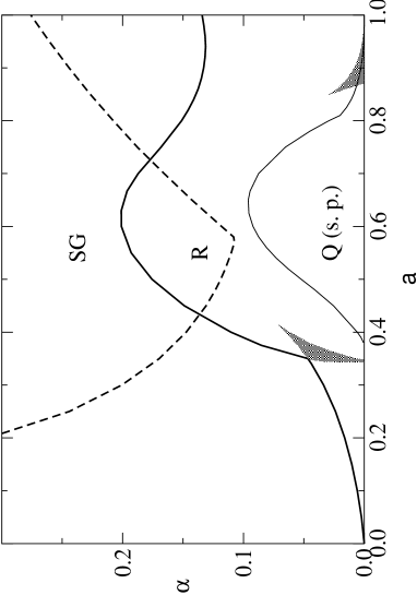
Figure 1: The capacity-activity $(\alpha-a)$ phase diagram for the BEG and $Q=3$-Ising networks at $T=0$. The meaning of the regions and of the lines is explained in the text.

There is a stable retrieval phase below the heavy solid line and a second retrieval phase with a smaller overlap appears in the lower shaded triangular regions. The pattern-fluctuation retrieval states are only saddle-point solutions below the light solid line. There is also everywhere a stable spin-glass solution and all the lines denote discontinuous transitions. For comparison, the heavy dashed line shows the retrieval phase boundary for the optimal three-state Ising layered network, optimal in the sense that the adjustable threshold parameter $\theta$ was chosen to optimize the storage capacity $\alpha$. Clearly, for intermediate activity $a\in(0.435,0.727)$ the BEG network has a larger critical storage capacity than the Ising network [16].

Another performance measure is the information content $i$ of the network and in Figs. 2 we show the information-capacity diagrams for various activities, at $T=0$, for the BEG and Ising networks. Again, the BEG performance is better for intermediate activity and the information content is purely due, at this temperature, to the only stable retrieval phase. At larger activity, $a=0.8$ say, the BEG and Ising networks compete for better performance at intermediate or larger $\alpha$ values, as seen in Fig. 2c.

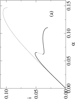
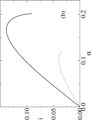
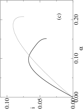
Figure 2: The mutual information $i$ as a function of the capacity $\alpha$ for the BEG (solid line) and the Q=3-Ising (dotted line) networks for $T=0$ and $a=0.4$ (a) $a=0.6$ (b) and $a=0.8$ (c).

In order to highlight the role of the temperature and the activity in the appearance of a stable $Q$ phase, we consider the temperature dependence for given activities and show in Fig. 3a the temperature-capacity diagram for $a=0.4$ and in Fig. 3b for $a=0.8$. In the first one there is only a stable retrieval phase (a second one in the shaded area) below the heavy phase boundary, in addition to the spin-glass phase. There are no $Q$ states, even not saddle-point solutions, in this region. In the case of $a=0.8$, instead, there is a single stable retrieval phase below the solid (dotted) heavy lines which denote discontinuous (continuous) transitions, respectively, with a tricritical point at $T\approx 0.753$ and $\alpha\approx 0.018$. There is also a stable (unstable saddle-point) $Q$ phase above (below) the heavy lines, as indicated in the figure, and the $Q$ phase solutions end at discontinuous transitions shown as solid light lines. There is also everywhere a stable spin-glass solution which only disappears as $T\rightarrow\infty$. It is clear from Fig. 3b that a stable $Q$ phase will only appear for sufficiently large synaptic noise and large activity, a feature also found for the extremely diluted [7] and the fully connected network [2].

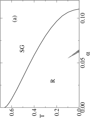
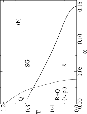
Figure 3: The temperature-capacity $(T,\alpha)$ phase diagram for the BEG network for $a=0.4$ (a) and $a=0.8$ (b). The meaning of the regions and lines are explained in the text.

We consider now the role of the activity and show the capacity-activity phase diagrams in Fig. 4a, for $T=0.4$, and in Fig. 4b, for $T=0.8$. In the case of the former there is a stable retrieval phase below the heavy solid line and a second stable retrieval phase in the shaded region. Again, there is a considerably enhanced storage capacity for retrieval, $\alpha\approx 0.119$, for an intermediate activity of $a\approx 0.676$. The pattern-fluctuation retrieval states are only saddle-point solutions and this is the case below the light solid line. When $T=0.8$ there is a stable retrieval phase below the heavy dotted (continuous transition) and heavy solid (discontinuous transition) lines which merge at a tricritical point at $a\approx 0.839$ and $\alpha\approx 0.0036$. The pattern-fluctuation retrieval solution is a stable phase below the light solid line and only a saddle point below the heavy and light dotted lines. There is now a finite storage capacity, $\alpha\approx 0.022$, at $a\approx 0.8$ for the retrieval of active patterns as a pattern-fluctuation retrieval phase.

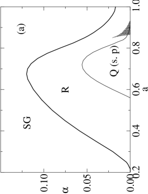
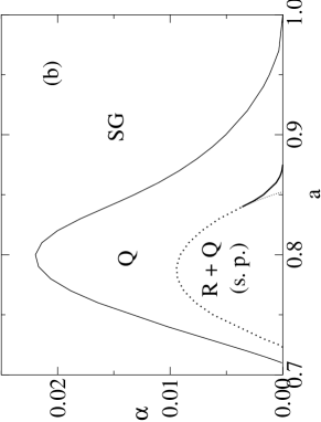
Figure 4: The capacity-activity $(\alpha,a)$ phase diagram for the BEG network at $T=0.4$ (a) and $T=0.8$ (b). The lines are explained in the text.

Thus, as $T$ increases, the useful performance of the network goes over from the retrieval to the pattern-fluctuation retrieval phase. Since the information content is a common performance measure for both phases, we show its temperature dependence in an information-capacity phase diagram in Fig. 5, for $a=0.8$ and various $T$, where the solid (dotted) lines represent information due to a stable retrieval (pattern-fluctuation retrieval) phase.

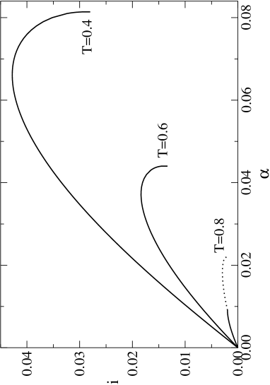
Figure 5: The information $i$ as a function of the capacity $\alpha$ for several values of $T$ and $a=0.8$.The solid (dashed) line correspond to the $R$ ($Q$) states.

In all the above situations the $SG$ solutions appear as a stable phase, and we consider now the flow diagrams in the $(l,m)$ order-parameter space. We show the results for $T=0.8$, activity $a=0.8$ for $\alpha=0.005$ in the presence of an $R$ phase in Fig. 6a, and for $\alpha=0.01$ in the presence of a $Q$ phase in Fig. 6b. These correspond to states on either side of the dotted phase boundary in Fig. 3b. In the first one there is a stable retrieval solution and there are two $Q$ saddle points (open circles) and in the second one there is a stable and an unstable $Q$ solution. In both cases there is a stable $SG$ solution which can be accessed only below the lower $Q$ saddle point. The chains of dots actually indicate time steps and, as can be seen from these figures, the flows to the stable solutions are considerably delayed by the saddle points in the form of slow transients of the dynamics. A remarkable feature of the flow diagrams is the presence of quite large basins of attraction either to the stable $R$ state or to the stable $Q$ state, even for the fairly high $T$ (and small $\alpha$) for this case. Also, not surprisingly, one finds a much smaller basin of attraction to the $SG$ states. Similar features have also been found in the dynamics of the extremely diluted network except for the $SG$ states, which are absent in that case [7].

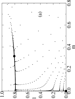
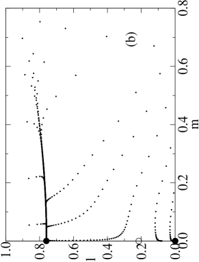
Figure 6: Two dimensional retrieval fluctuation overlap $l-m$ flow diagrams for the BEG network for $T=0.8$, $a=0.8$ and $\alpha=0.005$ (a) and $\alpha=0.01$ (b). Open circles are saddle points, closed ones are attractors.

We turn now to a brief study of the way in which the phase diagrams for the layered BEG network turn into those for the extremely diluted network by means of a variable amplitude $D$ in the second terms in Eq. (27), i.e.,

$$(\Delta^{t+1})^{2}=\alpha A^{2}q_{0}^{t}+D(\chi^{t})^{2}(\Delta^{t})^{2}\,\,,\quad(\Omega^{t+1})^{2}=\alpha B^{2}q_{0}^{t}+D(\psi^{t})^{2}(\Omega^{t})^{2}\,\,\,.$$ (28)

When $D=0$ we have the extremely diluted architecture, $D=1$ corresponds to the layered one. To be specific, consider the phase diagram for the layered network at $T=0.8$ shown in Fig. 4b where the phase boundary for existence of a stable $Q$ phase ends at $\alpha=0$ when the activity $a=1$. As $D$ decreases from unity, this part of the phase boundary moves up and the critical $\alpha$ gradually increases at $a=1$. For $D=0.9$ it becomes already $\alpha\approx 0.034$. At the same time the maximum activity $a$ for the lower retrieval phase boundary to a stable $R$ phase starts to increase towards larger values. The phase boundary itself continues to end at $\alpha=0$. For $D=0.5$, say, the maximum $a$ for retrieval is still less than unity and the $SG$ phase becomes now restricted to a region on both sides of the left phase boundary in the $\alpha$ vs. $a$ phase diagram. Ultimately, when the extremely diluted limit is reached, the stable $R$ phase goes up to $a=1$, still with $\alpha=0$, with a fairly large $Q$ phase and the $SG$ phase becomes a self-sustained activity phase $S$, with $m=0$, $l=0$ and $q_{1}=0$. In part of the phase diagram the $S$ and $Q$ phases coexist, in accordance with our earlier results on the extremely diluted network [7].

5 Concluding remarks

We have derived the recursion relations that describe the time evolution of the macroscopic variables for an exactly solvable three-state network on a feed-forward layered architecture, optimizing the mutual information. This so-called layered Blume-Emery-Griffiths (BEG) network shows distinct stationary phase diagrams from either its extremely diluted or fully connected versions studied in the literature. Being a truly dynamical system, there is no phase boundary of local stability in the layered network between either the retrieval, $R$, or the pattern-fluctuation retrieval phase, $Q$, and the spin-glass phase, $SG$, in contrast to the behavior in the fully connected network. But this does not mean that within the retrieval regime the network cannot be trapped in $SG$ states, as it is clear from the flow diagrams. This makes the layered network different from the extremely diluted network in which the $R$ or $Q$ states are the only stable states over most of the regions where these phases exist.

We have found that, in common with both the extremely diluted and the fully connected network, a stable pattern-fluctuation retrieval phase appears only at high $T$ and for intermediate-to-large, but not full, activity $a$. At low $T$, in particular at $T=0$, this phase is not stable but is instead a saddle-point solution. Nevertheless, the BEG layered network has, selectively, a quite better performance than the three-state Ising layered network, not only as far as the retrieval capacity is concerned, as in the case of both the fully connected and the extremely diluted network, but it also yields a considerably larger information content. This additional information is due to the enhancement by the pattern-fluctuation states of the stable retrieval phase at low and intermediate $T$. The pattern-fluctuation retrieval phase, instead, is responsible for a much smaller but non-negligible information content.

To summarize, the BEG network on a feed-forward layered structure is not only an interesting dynamical system in itself but it also performs better than other, for instance, Ising layered networks within relevant regimes of temperature and activity.

References

- [1] D. R. Carreta Dominguez and E. Korutcheva, Phys. Rev. E 62, 2620 (2000).
- [2] D. Bollé and T. Verbeiren, Phys. Lett. A 297, 156 (2002).
- [3] J.J.Hopfield, Proc. Nat. Acad. Sci. USA 79, 2554 (1982).
-
[4]
M. Blume, V. J. Emery and R. B. Griffiths, Phys. Rev. A 4, 1071 (1971);
M. Blume, Phys. Rev. 141, 517 (1966);
H. W. Capel, Physica 32, 966 (1966). - [5] J. M. de Araújo, F. A. da Costa and F. D. Nobre, Eur. Phys. J. B 14, 661 (2000).
- [6] D. R. C. Dominguez, E. Korutcheva, W. K. Theumann, and R. Erichsen Jr., in Lecture Notes in Computer Science (Springer, Berlin) 2415, 129 (2002).
- [7] D. Bollé, D. R. Dominguez, R. Erichsen, Jr., E. Korutcheva and W. K. Theumann, cond-mat/0208281 .
- [8] D. Bollé and T. Verbeiren, J. Phys. A 36, 295 (2003).
- [9] D. Bollé, J. Busquets Blanco and G. M. Shim, Physica A 318, 613 (2003).
- [10] D. Bollé, J. Busquets Blanco , G. M. Shim and T. Verbeiren, cond-mat/0304553
- [11] J. S. Yedidia, J. Phys. A 22, 2265 (1989).
- [12] D. Bollé, G. M. Shim, B. Vinck, and V. A. Zagrebnov, J. Stat. Phys. 74, 565 (1994).
- [13] D.L. Schacter, K.A. Norman and W. Koutstaal, Annu. Rev. Psychol. 49, 289 (1998).
- [14] E. Barkai, I. Kanter and H. Sompolinsky, Phys. Rev. A 41, 590 (1996).
- [15] E. Domany, W. Kinzel and R. Meir, J. Phys. A 22, 2081(1989).
- [16] D. Bollé, G. M. Shim and B. Vinck, J. Stat. Phys. 74, 583 (1994).
- [17] D. Bollé and D. Dominguez Carreta, Physica A 286, 401(2000).
- [18] D. R. C. Dominguez and D. Bollé, Phys. Rev. Lett. 80, 2961 (1998).
- [19] M. Okada, Neural Netw. 9, 1429 (1996).
- [20] C. E. Shannon, Bell Syst. Techn. J. 27, 379 (1948).
- [21] R. E. Blahut, Principles and Practice of Information Theory (Addison-Wesley, Reading, MA 1990), Chapter 5.