Phase field approach for modeling intracellular dynamics

Abstract

We introduce a phase field approach for diffusion inside and outside a closed cell with damping and with source terms at the interface. The method is compared to exact solutions (where possible) and the more traditional finite element method. It is shown to be very accurate, easy to implement and computationally inexpensive. We apply our method to a recently introduced model for chemotaxis by Rappel et al. [Biophys. J. 83, 1361 (2002)].

In dealing with free boundary problems, the so called phase field approach pf appears as a method of choice. It has successfully been applied to various problems ranging from dendritic solidification kr98 , viscous fingering pf-hs and crack propagation pf-crack . In the spirit of time-dependent Ginzburg-Landau models, the method avoids the tracking of the interface by introducing an auxiliary field that locates the interface and whose dynamics is coupled to the other physical fields through an appropriate set of partial differential equations. In comparison to the more traditional boundary integral methods, the method is much simpler to implement numerically.

In this Brief Report we introduce a phase field model for intracellular dynamics i.e. diffusion inside and outside a stationary, closed domain with source terms at the interface. We apply the method to a recently introduced model for the response of a Dictyostelium amoeba bill following stimulation with the chemoattractant cAMP rltl02 . In rltl02 , due to the need to use a finite element method the numerical implementation of the model was limited to two space dimensions and the cells were treated as disks. As we will see below, the phase field method is capable of faithfully capturing no-flux boundary conditions. Thus, it becomes feasible to investigate more realistic cell shapes in three dimensions.

Before we introduce our approach, we like to point out some possible extensions of our methodology. The phase field approach can be easily modified to include problems where the domain boundary is not stationary. For example, force generation on cell membranes, leading to shape changes, can be incorporated within the phase field approach in a straightforward manner. This would require adding an additional equation for the phase field, but does not require the explicit calculation of a boundary. We should stress that attempting to model this type of problem using conventional techniques, with explicit boundary tracking, become quite cumbersome.

Let us first introduce the most salient ingredients of our method. Our purpose is to describe the situation where some chemoattractant diffuses only inside the cell, i.e. its concentration $c$ obeys the diffusion equation inside a closed domain:

$$\frac{\partial c}{\partial t}=D\vec{\nabla}^{2}c$$

and satisfies zero-flux boundary conditions:

$$\hat{n}\cdot\vec{\nabla}c=0$$

As a phase field we take a function that takes the value $\phi_{in}=1$ inside the cell and $\phi_{out}=0$ outside the domain and varies smoothly across the interface. A possible choice in one dimension for a cell between $x=-a$ and $x=a$ is:

$$\phi(x)=\frac{1}{2}+\frac{1}{2}\tanh((a-|x|)/\xi)$$ (1)

The variable $\xi$ denotes the interface width. We then define a field $u$ that is to obey the equation:

$$\phi\frac{\partial u}{\partial t}=\vec{\nabla}\cdot\left[D\phi\vec{\nabla}u\right]$$ (2)

Our claim is now that inside the domain the field $u$ behaves very similarly to $c$. Let us therefore first show, for simplicity in one dimension, that in the thin interface limit one recovers the no-flux boundary condition. Integration of (2) over the interface yields:

$$\int_{a-\xi}^{a+\xi}dx\phi\frac{\partial u}{\partial t}\approx-D\frac{\partial u}{\partial x}\Big{|}_{x=a-\xi}$$

since $\phi(a-\xi)\approx 1$ and $\phi(a+\xi)\approx 0$. From this we deduce:

$$\frac{\partial u}{\partial x}\Big{|}_{x=a}\sim\xi$$

and thus, in the sharp interface limit $\xi\rightarrow 0$, the reflective boundary conditions are recovered. It is also clear that inside the domain where $\phi$ is constant $u$ satisfies the diffusion equation.

Another interesting property of Eq. (2) is that the quantity $\int\phi u\,d\vec{x}$, which can be interpreted as the total concentration inside the cell, is conserved under the dynamics. Thus, even if the field $u$ may become non-zero outside the cell (and indeed it does), the total concentration inside the cell remains constant. In fact, the asymptotic solution of Eq. (2) (together with phase field Eq. (1)) is $u(x)=A$ where the constant $A$ is determined through $2aA=\int dx\phi u(t=0)$. The real asymptotic solution is of course $u(x)=\tilde{A}=\int_{-a}^{a}dxu(t=0)/(2a)$. Because $\phi=1$ inside the domain and $\phi=0$ outside of it, the error $\cal E$ in the asymptotic solution depends solely on the amount of concentration initially near the interfaces: ${\cal E}\approx\int_{\pm a-\xi}^{\pm a+\xi}dx\phi u(t=0)/2a$. Since $\phi$ is an antisymmetric function around the interface, the error is minimal if we take in the phase field approach an initial condition $u(t=0)$ which is locally symmetric around the boundary.

This raises the following important point. While the solution $u$ outside the cell is not of physical interest, it is essential to keep track of it. In practice we solve (2) where the phase field $\phi$ exceeds a small threshold $\delta$ (typically $\delta\sim 10^{-8}$).

As a first test for our model we now solve Eq. (2) numerically in two space dimensions. For the phase field we take here:

$$\phi(r)=\frac{1}{2}+\frac{1}{2}\tanh((r_{0}-r)/\xi)$$ (3)

where $r$ is the radius in polar coordinates. In the case of a radially symmetric initial condition we can compare the field $u$ to the analytic solution $v$ which is expressed in terms of the Bessel functions

$$v(r,t)=\sum_{n}a_{n}J_{n}(\lambda_{n}r)\textrm{e}^{-\lambda_{n}^{2}t}$$

where $\lambda_{n}$ is defined as the smallest number for which $J_{n}(\lambda_{n}a)=0$ and $a_{n}$ is the projection of the initial condition on the set of Bessel functions. We also compare both fields $u$ and $v$ with the solution $w$ of a finite element method obtained with MATLAB’s PDE Toolbox (The Mathworks, Natick, MA).

In Fig. 1a we show the spatial profile of the phase-field together with the exact solution at a given time. It can be seen that the agreement is excellent, with a relative error of less than $1\%$ (see insert). In Fig. 1b we show the fields $u$,$v$ and $w$ at three different points. Again the agreement is excellent.

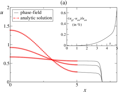
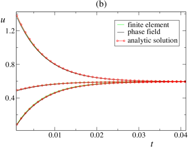
Figure 1: Comparison of our phase field model with both analytic solution and finite element method. The equations are solved on a grid of size $201\times 201$ with Euler’s method, with $D=250$, $r_{0}=5$, $\Delta x=0.1$, and $\Delta t=5\cdot 10^{-6}$. The initial condition is $c=1+\cos(\pi r/r_{0})$. (a) Spatial profile at respectively at $t=0.004$, $t=0.01$ and $t=0.02$ of the phase field and analytic solution. Since the curves are hardly distinguishable, we mark the analytic solution by small circles and plot the difference of the profiles at $t=0.01$ in the inset. The relative error of the phase field is seen to be smaller than 1%, being maximal at the boundary. (b) Time evolution of the concentration at $r=5$, $r=3.37$ and $r=1.66$. The analytic solution is again marked by small circles.

In view of these promising results, let us now consider diffusion in presence of a production term and damping. Including a source term at the interface is relatively easy. We add to the right hand side of (2) a term $b(\vec{\nabla}\phi)^{2}/\int d\vec{x}\,(\vec{\nabla}\phi)^{2}$. The factor $(\vec{\nabla}\phi)^{2}$ ensures that it only acts at the interface and the denominator is a normalization factor. To compensate for the production we also include a damping term of the form $-\mu\phi u$. The equation of motion then becomes:

$$\phi\frac{\partial u}{\partial t}=\vec{\nabla}\cdot\left[D\phi\vec{\nabla}u\right]-\mu\phi u+b\frac{(\vec{\nabla}\phi)^{2}}{\int d\vec{x}\,(\vec{\nabla}\phi)^{2}}$$ (4)

We have compared the phase field method with these two supplementary ingredients with the finite element method, again in the case of a two-dimensional circular cell with $r_{0}=5$. As can be seen in Fig. 2 the result is excellent.

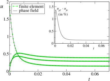
Figure 2: Comparison of our phase field model with finite element method with source and damping. We have taken the same system size, initial conditions and parameter values as in Fig. 1, and now $b=1000$ and $\mu=50$. We show here the time evolution of the concentration at $r=5$, $r=4.05$ and $r=0.86$. The curves are again hardly distinguishable. We plot the error $u_{pf}-u_{fe}$ for $r=5$ (the worst point of Fig.1a) as a function of time. As one can see in the insert, the error goes initially rapidly up to around 1.5 $\%$, but decreases then to around $6\cdot 10^{-2}\%$.

We now use our phase field method to solve a biological model for the response of a Dictyostelium amoeba following stimulation with the chemoattractant cAMP rltl02 . In recent experiments the establishment of an asymmetry within a few seconds after a rise of extracellular cAMP was demonstrated. The cAMP however diffuses rapidly around the cell and the applied signal is several orders of magnitude larger than the value required to elicit a response. This strongly suggests the presence of an inhibitory mechanism that suppresses responses at the back.

In rltl02 an abstract model for the initial response of the cell to the chemoattractant was proposed: it was supposed that the membrane can be characterized in terms of three states: quiescent (with density $\rho_{q}$), activated (with density $\rho_{a}$) and inhibited (with density $\rho_{i}$). Initially the entire membrane is in the quiescent state. As the cAMP reaches the front of the cell the membrane becomes activated at rate $\alpha[{\rm cAMP}]$ and an inhibitor, in rltl02 suggested to be cGMP, is produced (at rate $\sigma_{g}\rho_{a}$). The inhibitor diffuses toward the back of cell where it turns the membrane from quiescent to inhibited with rate $\beta_{r}[{\rm cGMP}]$. Furthermore both activated and inhibited state decay spontaneously to the quiescent state at rates $\delta$ and $\beta_{f}$ respectively. The equations for the membrane state variables are thus:

$$\frac{\partial\rho_{q}}{\partial t} = -\alpha c\rho_{q}+\beta_{f}\rho_{i}-\beta_{r}g\rho_{q}$$ (5)

$$\frac{\partial\rho_{a}}{\partial t} = \alpha c\rho_{q}-\delta\rho_{a}$$ (6)

$$\frac{\partial\rho_{i}}{\partial t} = -\beta_{f}\rho_{i}+\beta_{r}g\rho_{q}+\delta\rho_{a}$$ (7)

The reactants cGMP and cAMP diffuse respectively inside and outside the cell. At the membrane they satisfy zero-flux boundary conditions. There is an source term for the cGMP field that accounts for the production of cGMP at the interface. Both cAMP and cGMP fields are damped at rates $\mu_{c}$ and $\mu_{g}$. The phase-field method is thus well suited to solve the dynamical equations for the cAMP and cGMP concentrations. For the phase field corresponding to the cAMP (which diffuses outside the cell) we simply take the complement of $\phi$ given by Eq. (3): $\phi_{c}=1-\phi$. The equations for the membrane variables are solved on all lattice sites where $(\vec{\nabla}\phi)^{2}$ exceeds a certain threshold, namely $10^{-4}$.

We now present a comparison of the phase field approach and the results obtained with a finite element method in rltl02 . A circular cell of diameter 10 $\mu$m is placed in a square domain of 30 $\mu$m by 30 $\mu$m. The diffusion constant of cAMP and cGMP was taken to be identical: $D_{c}=D_{g}=250\mu$m²/s. The values of the other parameters can be read in the caption of Fig.3.

In order to mimic the asymmetric cAMP stimulus we maintain the cAMP concentration at a value well above threshold at the upper left corner of our domain. As expected from our earlier results the agreement of the cAMP fields, that solely diffuse around the cell, is excellent, see Fig. 3a. We observe a slight discrepancy for the cGMP field (also Fig. 3a), which grows with time. This is related to the larger difference (of around 10%) for the membrane variables, the production of cGMP being proportional to $\rho_{a}$. The origin of the discrepancy might lie in the way the state variables are calculated: on a ring of finite width in the phase field model, and on 40 points on the interface in the finite element method. At any rate, since the model is of a quite abstract nature and since its predictions are only qualitative, a detailed investigation is beyond the scope of this paper.

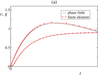
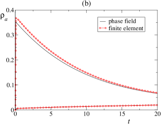
Figure 3: Comparison of our phase field model with finite element method in the chemotaxis model. (a) cGMP concentration at front (upper curves) and cAMP at back (lower curves) of the cell as a function of time (b) state variables $\rho_{a}$ at front and back of the cell as a function of time. In the finite element method the grid consists of 216 nodes inside the cell (of which 40 on the interface) and 543 on the outside (of which again 40 on the interface). The grid and also the mass and stiffness matrices were generated by MATLAB’s PDE Toolbox (The Mathworks, Natick, MA) after which the equations of motion are integrated with a Fortran code. The time step is taken to be $\Delta t=2\cdot 10^{-6}$. In the phase field method the equations of motion are integrated on a $151\times 151$ grid, the lattice spacing thus being $\Delta x=0.2$. Here the time step is taken to be $\Delta t=10^{-5}$. We have taken the following parameter values: $\alpha=4$ , $\beta_{f}=0.01$, $\beta_{r}=0.533$, $\delta=0.1$, $\mu_{c}=0$, $\mu_{g}=0.12$, and $\sigma_{g}=60000$.

From a computational perspective, we note that in the phase field method the CPU time required is linear in the number of lattice sites whereas it is quadratic in the number of nodes in the finite element method. One thus expects the phase field method to be much faster. However this naive result must be taken with some caution as in the finite element method the nodes are not distributed uniformly in space. To resolve some particular region in space with high accuracy we are thus obliged to take a small lattice spacing in the phase field method, such that the number of lattice points exceeds the number of nodes. Other parameters that will affect the accuracy of both methods are the time step $\Delta t$ and the integration algorithm. Again a detailed comparison is beyond the scope of the Report. In practice it turns out that the phase field method where the lattice spacing is equal to the minimal distance between two nodes of our finite element method is about one order of magnitude faster.

Finally, we turn to the chemotaxis model in three space dimensions. For the sake of simplicity we take a spherical cell, i.e. with a phase field like in Eq. (3) but where $r$ is now the radius in spherical coordinates. We consider again a cell of radius $r_{0}=5\mu m$, in a box of dimensions $30\times 30\times 30\mu m$. Now the stimulus is applied by setting the cAMP initially well above threshold at one side of the box, here taken to be $x=-15\mu m$. As is illustrated in Fig. 4, the phenomenology of the two dimensional case is reproduced here. As the cAMP front progresses toward the back of the cell, only the front of the cell is activated.

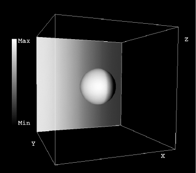
Figure 4: The cAMP concentration, represented by gray levels (where white corresponds to large concentrations and black to low ones) is for visual simplicity shown at the back of the box and is similar to the cAMP field surrounding the cell. The activity density of the membrane is shown on the sphere, also represented by gray levels. It is seen that whereas the cAMP has reached the back of the cell, it has not become activated. The equations of motion are integrated on a $61\times 61\times 61$ grid, the lattice spacing thus being $\Delta x=0.5$. Here the time step is taken to be $\Delta t=10^{-4}$. These results have been obtained for the same parameters as in Fig. 3. Only the production term has been increased in order to account for the increase in membrane surface.

In conclusion we have proposed a phase field model for intracellular dynamics. Our method is shown to be very accurate, easy to implement and computationally inexpensive. Another advantage lies in its much greater flexibility with respect to other methods, like the finite element method. We revisited a chemotaxis model and, when considering three dimensional cells, we reach the same conclusions as in rltl02 for two-dimensional cells. Whereas we have restricted ourselves to circular and spherical domains, the extension to other geometrical forms poses no major problems, the only task being to generate a phase field $\phi$. Even better, our approach can easily be extended to deal with non-stationary boundaries. This situation arises in a multitude of biological problems. For example, the Dictyostelium cells change their shape continuously during chemotaxis. Another example are shape transformations observed in vesicles seifert . In these cases, the phase field becomes a dynamic variable, that evolves under the appropriate Ginzburg-Landau type of equation. We are currently working along these lines of research.

This work was supported by the NSF sponsored Center for Theoretical Biological Physics (grants PHY-0216576 and 0225630) and the NSF Biocomplexity program (grant MCB 0083704).

References

- (1) W.J. Rappel, H. Levine, P.J. Thomas, W.F. Loomis Biophys. J. 83, 1361 (2002)
- (2) J.B. Collins and H. Levine, Phys.Rev.B 31, 6119 (1985), J.S. Langer in Directions in Condensed Matter, (World Scientific, Singapore, 1986)
- (3) A. Karma and W.-J. Rappel, Phys. Rev. E, 57, 4323 (1998)
- (4) R. Folch, J. Casademunt, A. Hernández-Machado and L. Ramírez-Piscina Phys. Rev. E, 60, 1724 (1999)
- (5) I.S. Aranson, V.A. Kalatsky, V.M. Vinokur, Phys. Rev. Lett. 85, 118 (2000) A. Karma, D.A. Kessler, H. Levine, Phys. Rev. Lett. 87, 045501 (2001)
- (6) W.F. Loomis, Dictyostelium Discoideum : A Developmental System (Academic Press, New York, 1975)
- (7) C.A. Parent, B.J. Blacklock, W.M. Foehlich, D.B. Murphy and P.N. Devreotes, Cell 95, 81 (1998)
- (8) U. Seifert Adv. Physics, 46, 13 (1997)