Instability of vortex array and transitions to turbulent states in rotating helium II

Abstract

We consider superfluid helium inside a container which rotates at constant angular velocity and investigate numerically the stability of the array of quantized vortices in the presence of an imposed axial counterflow. This problem was studied experimentally by Swanson et al., who reported evidence of instabilities at increasing axial flow but were not able to explain their nature. We find that Kelvin waves on individual vortices become unstable and grow in amplitude, until the amplitude of the waves becomes large enough that vortex reconnections take place and the vortex array is destabilized. The eventual nonlinear saturation of the instability consists of a turbulent tangle of quantized vortices which is strongly polarized. The computed results compare well with the experiments. Finally we suggest a theoretical explanation for the second instability which was observed at higher values of the axial flow.

I Introduction

The work described in this article is concerned with the stability of a superfluid vortex array. It is well knownDonnelly BDV2 that, if helium II is rotated at constant angular velocity $\Omega$, an array of superfluid vortex lines is created. The vortices are aligned along the axis of rotation and form an array with areal density given by

$$L_{rot}=\frac{2\Omega}{\kappa},$$ (1)

where $\kappa=h/m=9.97\times 10^{-4}{\rm cm^{2}/sec}$ is the quantum of circulation, $h$ is Plank’s constant and $m$ the mass of one helium atom. Equation (1) is valid provided that $\Omega$ exceeds a small critical valueFetter . Rotation frequencies of the order of $1~{}\rm Hz$ are easily achieved in a laboratory, and correspond to real density of the order of $10^{3}~{}\rm cm^{-2}$.

It is also well known that a superfluid vortex line becomes unstable in the presence of normal fluid in the direction parallel to the axis of the vortex. This instability, hereafter referred to as the Donnelly- Glaberson (DG) instability, was first observed experimentally by Cheng et al. Cheng and then explained by Glaberson et al. Glaberson . Physically, the DG instability takes the form of Kelvin waves (helical displacements of the vortex core) which grow exponentially with time.

In this paper we use an imposed axial flow to trigger the DG instability and study the transition from order to disorder in an array of quantized vortex lines. It is useful to remark here that, since the growth of Kelvin waves takes place at the expense of normal fluid’s energy, understanding the DG instability is also relevantSK to the balance of energy between normal fluid and superfluid in helium II turbulence, a problem which is attracting current experimental Stalp Tabeling Lancaster1 Lancaster2 and theoreticalABC BHS Tsubota Vinen1 attention.

The article is organized in the following way. In section 2 we describe the rotating counterflow configuration, which is relevant to both theory and experiment. In section 3 we summarize experimental results obtained by Swanson, Barenghi and DonnellySwanson . They discovered that the DG mechanism can destabilize the superfluid vortex array and revealed the existence of two different superfluid states at increasing values of the driving axial flow beyond the DG transition. Until now, the actual physical nature of these two states has been a mystery, and it is the aim of our work to shed light into this problem. In section 4 we set up the formulation of vortex dynamics in the rotating frame which generalizes the previous approach of Schwarz Schwarz and which we use in our numerical calculations. Section 5 is devoted to the DG instability. What happens beyond the DG instability cannot be predicted by linear stability theory and must be investigated by direct nonlinear computation, which is done in section 6. In section 7 we tackle the transition to the second turbulent state observed by Swanson et al. Finally, section 8 draws the conclusions.

II Rotating counterflow

In order to study the stability of the rotating superfluid vortex array, we consider the configuration which is schematically shown in Fig. 1. A channel, which is closed at one end and open to the helium bath at the other end, is placed on a table which can be rotated at an assigned angular velocity $\Omega$. At the closed end of the channel a resistor dissipates a known heat flux $\dot{Q}$.

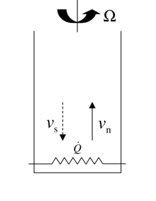
Figure 1: Schematic rotating counterflow apparatus.

First let us consider what happens in the absence of rotation ($\Omega=0$). Since only the normal fluid carries entropy, then $\dot{Q}=\rho TSV_{n}$, where $T$ is the absolute temperature, $S$ the specific entropy, $\rho=\rho_{s}+\rho_{n}$ the total density of helium II, $\rho_{s}$ the superfluid density and $\rho_{n}$ the normal fluid density. We call $V_{n}$ and $V_{s}$ respectively the normal fluid and the superfluid velocity fields in the direction along the channel, averaged over the channel’s cross section. The total mass flux $\rho_{s}V_{s}+\rho_{n}V_{n}$ is zero because one end of the channel is closed. The resulting counterflow velocity $V_{ns}=V_{n}-V_{s}$ which is induced along the channel is therefore proportional to the applied heat flux:

$$V_{ns}=\frac{\dot{Q}}{\rho_{s}ST}$$ (2)

It is known from experimentsTough Vinen2 and numerical simulations Schwarz that, if $\dot{Q}$ (hence $V_{ns}$) exceeds a critical value, a turbulent tangle of quantized vortex lines is created. The tangle is homogeneous and isotropic (neglecting a small degree of anisotropy induced by the direction of the imposed hear current). The intensity of the turbulence is measured by the vortex line density (length of vortex line per unit volume) which is experimentally determined by monitoring the extra attenuation of second sound. It is found that the vortex line density has the form

$$L_{\rm flow}=\gamma_{H}^{2}V_{\rm ns}^{2},$$ (3)

where $\gamma_{H}$ is a temperature dependent coefficient Tough .

Let us consider now the case in which the heat flux is applied in the rotating frame ($\Omega\neq 0$). We have now two effects which compete with each other: rotation, which favours the creation of an ordered array of vortices aligned along the direction of the axis of rotation, and counterflow, which favours the creation of a disordered tangle. Swanson et al.Swanson were the first to address the problem of whether the vortex array is stable or not at given values of $\Omega$ and $V_{ns}$, and, if the array is unstable, of whether the vortex line density $L$ is the sum of Eq. (1) and Eq. (3) or not. Their experimental results are described in the next section.

It is important to remark that, in principle, one can also study the stability of a vortex array in the presence of a mass flow rather than of a heat current. Similarly, one can study the effects of rotation upon the turbulence of helium II created by towing a grid or rotating a propellers rather than upon counterflow turbulence. The reason for which we have chosen to restrict our investigation to the case of a heat current is twofold: firstly, the experimental data of Swanson et alSwanson are available; secondly, at least at small heat currentsMelotte , the turbulent superfluid tangle is homogeneous and almost isotropic and we do not have to worry about large scale motion and eddies of the normal fluid.

III The experiment

The rotating counterflow apparatus of Swanson et al Swanson consisted of a $40~{}\rm cm$ long vertical channel with $1\times 1~{}\rm cm^{2}$ square cross section. At the closed end (as shown in Fig. 1) a resistor dissipated a known heat flux $\dot{Q}$ and induced relative motion $V_{ns}$ of the two fluid components. The vortex line density $L$ was measured by pairs of second sound transducers located along the channel. The entire apparatus was set up on a rotating cryostat, so that it was possible to create vortex lines by either rotation or counterflow, or by any combination of them. The vortex line density was calculated from a measurement of the attenuation of second sound resonances and its calibration against the known density in rotation BPD .

The experiment was performed at $T=1.65~{}\rm K$. In the presence of both rotation and counterflow three distinct flow states were observed, as shown in Fig. 2. The three states are separated by two critical counterflow velocities $V_{c1}$ and $V_{c2}$, which are respectively the boundaries between the primary state and the secondary state, and between the secondary state and the tertiary state. The results of the experiment can be summarized as it follows:

$\bullet$ Primary state

In the first region of Figure 2 at the left of $V_{c1}$ the vortex line density is independent of the small values of $V_{ns}$ involved and agrees with Eq. (1). This region clearly corresponds to an ordered vortex array, and the counterflow current $V_{ns}$ is not strong enough to destabilize it.

$\bullet$ Transition from primary state to secondary state

Swanson et al. Swanson noticed that the values of the first critical velocity $V_{c1}$ are consistent with the DG instability. This means that at $V_{ns}=V_{DG}$ the axial flow is so strong that Kelvin waves of infinitesimal amplitude become unstable.

$\bullet$ Secondary state

Because of the lack of direct flow visualization in helium II, the nature of the flow past the instability ($V_{ns}>V_{c1}$) was not clear to Swanson et al Swanson . The only information which they could recover by the second sound measurement technique was that rotation added fewer than the expected $2\Omega/\kappa$ vortex lines to those made by the counterflow current.

$\bullet$ Transition from secondary state to tertiary state

The existence of a second critical velocity $V_{c2}$ was unexpected. The nature of the transition at $V_{ns}=V_{c2}$ and which kind of flow exists in the third region ($V_{ns}>V_{c2}$) were a mystery.

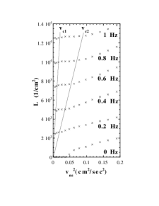
Figure 2: Vortex line density $L$ observed by Swanson et al. Swanson in the presence of a counterflow heat current $V_{ns}$ at various rotation rates at $T=1.65$. The solid lines represent fits to the two observed critical velocities $V_{c1}$ and $V_{c2}$. The experimental uncertainties are about $1/3$ of the symbol size.

IV Vortex dynamics in a rotating frame

The vortex filament model is very useful to study the motion of superfluid ⁴He because the vortex core radius $a_{0}\sim 10^{-8}$ cm is microscopic, hence much smaller than any flow scales of interest. Moreover, unlike what happens in classical fluid dynamics, the circulation $\kappa=9.97\times 10^{-4}$ cm²/sec is fixed by quantum constraint, which simplifies the model ever further.

Helmholtz’s theorem for a perfect fluid states that a vortex moves with self - induced velocity at each place produced by the shape of the vortex itself. Therefore the velocity $\dot{\vec{s}}_{0}$ of a vortex filament at the point $\vec{s}$ in the absence of mutual friction is governed by the Biot-Savart law and can be expressed as Schwarz :

$$\dot{\vec{s}}_{0}=\frac{\kappa}{4\pi}\vec{s}^{\prime}\times\vec{s}^{\prime\prime}\ln\left(\frac{2(l_{+}l_{-})^{1/2}}{e^{1/4}a_{0}}\right)+\frac{\kappa}{4\pi}\int^{\prime}\frac{(\vec{s}_{1}-\vec{r})\times d\vec{s}_{1}}{|\vec{s}_{1}-\vec{r}|^{3}}.$$ (4)

Here the vortex filament is represented by the parametric equation $\vec{s}=\vec{s}(\xi,t)$. The first term means the localized induction velocity, where the symbols $l_{+}$ and $l_{-}$ are the lengths of the two line elements which are adjacent to a given point after discretization of the filament, and the prime denotes differentiation of ${\vec{s}}$ with respect to the arc length $\xi$. The second term represents the nonlocal field obtained by carrying out the integral along the rest of the filament on which $\vec{s}_{1}$ refers to a point.

If the temperature is finite, the normal fluid fraction is non-zero and its effects must be taken into account. The normal fluid induces a mutual friction force which drags the vortex core of a superfluid vortex filament for which the velocity of point $\vec{s}$ is given by

$$\dot{\vec{s}}=\dot{\vec{s}}_{0}+\alpha\vec{s}^{\prime}\times(\vec{v}_{\rm ns}-\dot{\vec{s}}_{0})-\alpha^{\prime}\vec{s}^{\prime}\times[\vec{s}^{\prime}\times(\vec{v}_{\rm ns}-\dot{\vec{s}}_{0})],$$ (5)

where $\alpha$ and $\alpha^{\prime}$ are known temperature-dependent friction coefficients and $\dot{\vec{s}}_{0}$ is calculated from Eq. (4). More details of the numerical method and how it is implemented are described in Ref.TAN .

In order to make progress in our problem, we need to generalize this vortex dynamics approach to a rotating frame Yoneda . The natural way to perform the calculation in a rotating frame would require to consider a cylindrical container. We do not follow this approach for two reasons. Firstly, our formulation is implemented using the full Biot - Savart law, not the localized-induction approximation often used in the literature. This would require to place image vortices beyond the solid boundary to impose the condition of no flow across it. This is easily done in cartesian (cubic) geometry, but it is difficult to do in cylindrical geometry, Secondly, the original experiment by Swanson et al. Swanson was carried out in a rotating channel with a square cross section.

In a rotating vessel the equation of motion of vortices is modified by two effects. The first is the force acting upon the vortex due to the rotation. According to the Helmholtz’s theorem, the generalized force acting upon the vortex is balanced by the Magnus force:

$$\rho_{\rm s}\kappa(\vec{s}^{\prime}\times\dot{\vec{s}}_{0})=\frac{\delta F^{\prime}}{\delta\vec{s}},$$ (6)

where $F^{\prime}=F-\vec{\Omega}\cdot\vec{M}$ is the free energy of a system in a frame rotating around a fixed axis with the angular velocity $\vec{\Omega}$ and the angular momentum $\vec{M}$. Taking the vector product of Eq.(6) with $\vec{s}^{\prime}$, we obtain the velocity $\dot{\vec{s}}_{0}$. The first term $F$ due to the kinetic energy of vortices gives that Biot - Savart law, and the second term $\vec{\Omega}\cdot\vec{M}$ leads to the velocity $\dot{\vec{s}}_{\rm rot}$ of the vortex caused by the rotation:

$$\dot{\vec{s}}_{\rm rot}=\frac{1}{4\pi} \int \left\{3\frac{\vec{s}^{\prime}\times\vec{R}}{|\vec{R}|^{5}}[(\vec{\Omega}\cdot\vec{s}^{\prime})(\vec{r}\cdot\vec{R})-(\vec{\Omega}\cdot\vec{R})(\vec{r}\cdot\vec{s}^{\prime})]\right.$$ (7)

$${}+\frac{\vec{s}^{\prime}\times\vec{\Omega}}{|\vec{R}|^{5}}[|\vec{R}|^{2}(\vec{r}\cdot\vec{s}^{\prime})-3(\vec{r}\cdot\vec{R})~{}(\vec{R}\cdot\vec{s}^{\prime})]$$

$${}-\frac{\vec{s}^{\prime}\times\vec{r}}{|\vec{R}|^{5}}[|\vec{R}|^{2}(\vec{\Omega}\cdot\vec{s}^{\prime})-3(\vec{\Omega}\cdot\vec{R})~{}(\vec{R}\cdot\vec{s}^{\prime})]$$

$${}\left.-\frac{\vec{\Omega}\times\vec{r}}{|\vec{R}|^{3}}+\frac{\vec{s}^{\prime}\cdot(\vec{\Omega}\times\vec{r})}{|\vec{R}|^{3}}\vec{s}^{\prime}\right\}d\vec{r}$$

with $\vec{R}=\vec{r}-\vec{s}$. The second effect is the superflow induced by the rotating vessel. For a perfect fluid we know the analytical solution of the velocity inside a cube of size $D$ rotating with the angular velocity $\vec{\Omega}=\Omega\hat{\vec{z}}$ Thomson :

$$\vec{v}_{{\rm cub},x} = \frac{8\Omega}{\pi^{2}}\sum_{n=0}^{\infty}\frac{(-1)^{n}}{(2n+1)^{2}}\frac{D}{2}{\rm sech}\frac{(2n+1)\pi}{2}$$ (8)

$${}\times\left[{\rm sinh}Y{\rm cos}X-{\rm cosh}X{\rm sin}Y\right]$$

$$\vec{v}_{{\rm cub},y} = \frac{8\Omega}{\pi^{2}}\sum_{n=0}^{\infty}\frac{(-1)^{n}}{(2n+1)^{2}}\frac{D}{2}{\rm sech}\frac{(2n+1)\pi}{2}$$ (9)

$${}\times\left[{\rm cosh}Y{\rm sin}X-{\rm sinh}X{\rm cos}Y\right]$$

with $X=(2n+1)\pi x/D$ and $Y=(2n+1)\pi Y/D$. In a rotating frame these terms are added to the velocity $\dot{\vec{s}}_{0}$ without the mutual friction, so Eq. (4) is replaced by

$$\dot{\vec{s}}_{0} = \frac{\kappa}{4\pi}\vec{s}^{\prime}\times\vec{s}^{\prime\prime}\ln\left(\frac{2(l_{+}l_{-})^{1/2}}{e^{1/4}a_{0}}\right)+\frac{\kappa}{4\pi}\int^{\prime}\frac{(\vec{s}_{1}-\vec{r})\times d\vec{s}_{1}}{|\vec{s}_{1}-\vec{r}|^{3}}$$ (10)

$${}+\dot{\vec{s}}_{\rm rot}+\vec{v}_{\rm cub}.$$

Some important quantities useful for characterizing the rotating tangle will be introduced. The vortex line density is

$$L=\frac{1}{\Lambda}\int d\xi,$$ (11)

where the integral is made along all vortices in the sample volume $\Lambda$. The polarization of the tangle may be measured by the quantity

$$<s^{\prime}_{z}>=\frac{1}{\Lambda L}\int d\xi\vec{s}^{\prime}(\xi)\cdot\hat{\vec{z}},$$ (12)

as a function of time.

The actual numerical technique used to perform the simulation has been alreay describedTAN . Here it is enough to say that a vortex filament is represented by a single string of points at a distance $\Delta\xi$ apart. When two vortices approach within $\Delta\xi$, they are assumed to reconnectKoplik . The computational sample is taken to be a cube of size $D=1.0$ cm. We adopt periodic boundary conditions along the rotating axis and rigid boundary conditions at the side walls. All calculations are made under the fully Biot-Savart law, placing image vortices beyond the solid boundaries. The space resolution is $\Delta\xi=1.83\times 10^{-2}$ cm and the time resolution is $\Delta t=4.0\times 10^{-3}$ sec. All results presented in this paper refer to calculations made in the rotating frame. To make comparison with the experiment Swanson , we use $\alpha=0.1$ and $\alpha^{\prime}=0$ at the temperature $T=1.6$K. The uniform counterflow ${\vec{v}_{\rm ns}}$ is applied along the $z$ axis.

V The DG instability

Swanson et al. Swanson found that the first critical velocity $V_{c1}$ was proportional to $\Omega^{1/2}$; this functional dependence and the actual numerical values were consistent with interpreting the transition at $V_{ns}=V_{c1}$ as the DG instability of Kelvin waves. Glaberson et al. Glaberson considered an array of quantized vortices (which they modelled as a continuum) inside a container rotating at an angular velocity $\Omega$. They found that, in the absence of friction, the dispersion relation of a Kelvin wave of wavenumber $k$ is

$$\omega=2\Omega+\nu k^{2},$$ (13)

where $\omega$ is the angular frequency of the Kelvin wave, $\nu$ is given by

$$\nu=\frac{\kappa}{4\pi}\ln{(\frac{b}{a_{0}})},$$ (14)

where $b\approx L^{-1/2}$ is the average distance between vortices.

Glaberson et al. Glaberson showed that the dispersion law (13) has a critical velocity

$$V_{DG}=\frac{\omega}{k}_{min}=2(2\Omega\nu)^{1/2}$$ (15)

at the critical wavenumber

$$k_{DG}=\sqrt{\frac{2\Omega}{\nu}}.$$ (16)

If the axial flow $V_{\rm ns}$ exceeds $V_{DG}$ for some value of $k$, then Kelvin waves with that wavenumber $k$ (which are always present at very small amplitude due to thermal excitations and mechanical vibrations) become unstable and grow exponentially in time. Physically, the phase velocity of the mode $k$ is equal to the axial flow, so energy is fed into the Kelvin wave by the normal flow.

Figure 3 illustrates the DG instability. The computations were performed in a periodic box of size $1~{}\rm cm$ in a reference frame rotating with angular velocity $\Omega=9.97\times 10^{-3}~{}\rm rad/sec$, for which $V_{DG}=0.010~{}\rm cm/sec$. Figure 3a confirms that when $V_{ns}=0.008~{}\rm cm/sec<V_{DG}$ the vortex lines remain stable. Figure 3b shows that, at $V_{ns}=0.015~{}\rm cm/sec>V_{DG}$, Kelvin waves become unstable and grow, as predicted. Figures 3c,d,e and f show that Kelvin waves of larger wavenumber become unstable at higher counterflow velocity.

(a)                        (b)

(c)                        (d)

(e)                        (f)

Figure 3: Numerical simulations of the Donnelly-Glaberson instability at $\Omega=9.97\times 10^{-3}{\rm rad/sec}$, $T=1.6{\rm K}$. Snapshots of vortex configurations at the following counterflow velocities $V_{ns}$: (a): $V_{ns}=0.008{\rm cm/sec}$; (b): $V_{ns}=0.015{\rm cm/sec}$; (c): $V_{ns}=0.03{\rm cm/sec}$; (d): $V_{ns}=0.05{\rm cm/sec}$; (e): $V_{ns}=0.06{\rm cm/sec}$; (f): $V_{ns}=0.08{\rm cm/sec}$.

Linear stability theoryDrazin can only predict two quantities: the first is the critical value of the driving parameter ($V_{DG}$ in our case) at which a given state (the vortex array in our case) becomes unstable because infinitesimal perturbations grow rather than decay; the second is the exponential growth or decay rate of these perturbations for a given value of the driving parameter. Therefore the linear stability theory of GlabersonGlaberson cannot answer the question of what is the new solution which grows beyond the DG instability: to determine this new solution (what we call the secondary state in section 3) we must solve the governing nonlinear equations of motion, which is what we do in the next section.

VI Rotating turbulence

Because of the computational cost of the Biot-Savart law, it is not practically possible to compute vortex tangle with densities which are as high ($L={\cal O}(10^{4}){\rm cm^{-2}}$) as those achieved in the experiment. Nevertheless, numerical simulations performed at smaller, computationally realistic values of $L$ are sufficient to shed light into the physical processes involved. Some results which we describe have been already presented in preliminary formpreliminary ; together with more recent computer simulations, the picture which emerges and which we present here gives a good understanding of the experimental findings of Swanson et alSwanson , at least as far as the transition to the secondary flow and the secondary flow itself are concerned.

The time sequence contained in Fig. 4 illustrates the evolution of a vortex array at a relatively small angular velocity $\Omega=9.97\times 10^{-3}{\rm rad/sec}$, in the presence of the counterflow $V_{ns}=0.08{\rm cm/sec}$. Figure 4a shows the initial $N=8$ parallel vortex lines at $t=0$. The vortices have been seeded with small random perturbations to make the simulation more realistic. The absence of these perturbations would make the phase of the Kelvin waves synchronize on all vortices to delay reconnections. As the evolution proceeds, perturbations with high wavenumbers are damped by the mutual friction, whereas perturbations which are linearly DG-unstable grow exponentially, hence Kelvin waves become visible (Fig. 4b). When the amplitude of the Kelvin waves becomes of the order of the average vortex separation, reconnections take place (Fig. 4c). The resulting vortex loops disturb the initial vortex array, leading to an apparently random vortex tangle (Fig. 4d). After the initial exponential growth (which is predicted by the theory of the DG instability), nonlinear effects (vortex interactions and vortex reconnections) become important and nonlinear saturation takes place.

(a)                        (b)

(c)                        (d)

(e)                        (f)

Figure 4: Numerical simulation of rotating turbulence at $T=1.6{\rm K}$, $\Omega=9.97\times 10^{-3}{\rm rad/sec}$ and $V_{ns}=0.08{\rm cm/sec}$. Computed vortex tangle at the following times: (a): t=0rm sec; (b): t=16sec; (c): t=28sec; (d): t=36sec; (e): t=80sec; (f): t=600sec.

Figure 5 shows a similar time sequence at the same counterflow velocity $V_{ns}=0.08{\rm cm/sec}$ but at higher rotation rate $\Omega=4.98\times 10^{-2}{\rm rad/sec}$. In this case we have $N=33$ initial parallel vortices (Fig. 5a). At $t=12{\rm sec}$ (Fig. 5b) it is still $N=33$. Then the amplitude of the Kelvin waves becomes so large that lots of reconnections take place and $N$ increases; for example, we have $N=83$ at $t=160{\rm sec}$ (Fig. 5f).

(a)                        (b)

(c)                        (d)

(e)                        (f)

Figure 5: Numerical simulation of rotating turbulence at $T=1.6{\rm K}$, $\Omega=4.98\times 10^{-2}{\rm rad/sec}$ and $V_{ns}=0.08{\rm cm/sec}$. Computed vortex tangle at the following times: (a): t=0rm sec; (b): t=12sec; (c): t=20sec; (d): t=28sec; (e): t=40sec; (f): t=160sec.

It is instructive to compare these results with ordinary counterflow in the absence of rotation. Figure 6 shows a vortex tangle obtained for $\Omega=0$ and $V_{ns}=0.08{\rm cm/sec}$. The dynamics starts from $N=6$ vortex rings. It has been known since the early work of Schwarz Schwarz that the resulting tangle does not depend on the initial condition. In this particular simulation the vortices develop to a turbulent tangle.

(a)                        (b)

(c)                        (d)

(e)                        (f)

Figure 6: Numerical simulation of counterflow turbulence at $T=1.6{\rm K}$ in the absence of rotation ($\Omega=0$) for $V_{ns}=0.08{\rm cm/sec}$. Computed vortex tangle at the following times: (a): t=0rm sec; (b): t=120sec; (c): t=360sec; (d): t=520sec; (e): t=680sec; (f): t=1160sec.

Figure 7 shows that in all three cases (small rotation, large rotation, no rotation) the vortices, after an initial transient, saturate to a statistically steady, turbulent state, which is characterized by a certain average value of $L$. In the case of $\Omega\neq 0$ (Fig. 6a and b), it is apparent that the initial growth is exponential, which confirms the occurrence of a linear instability.

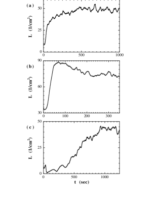
Figure 7: Vortex line density $L$ vs time $t$ at $T=1.6{\rm K}$ and $V_{ns}=0.08{\rm cm/sec}$ for: (a): $\Omega=9.97\times 10^{-3}{\rm rad/sec}$; (b): $\Omega=4.98\times 10^{-2}{\rm rad/sec}$; (c): $\Omega=0{\rm rad/sec}$.

Looking carefully at the saturated tangle at higher rotation (Fig. 5f) we notice that there are more loops oriented vertically than horizontally. The effect is not visible at lower rotation (Fig. 4f) and at zero rotation (Fig. 6f). The degree of polarization of the tangle is represented by $\ <s^{\prime}_{z}>$ of Eq.(12). This quantity captures the difference between a vortex array (for which $<s^{\prime}_{z}>=1$ because all lines are aligned in the $+z$ direction) and a random vortex tangle (for which $<s^{\prime}_{z}>=0$ because there is an equal amount of vorticity in the $+z$ and $-z$ directions). Figure 8 shows how $<s^{\prime}_{z}>$ changes with time in the three cases (small rotation, large rotation, no rotation) considered. The quantities of interest are the values of $<s^{\prime}_{z}>$ at large times in the saturated regimes. In the absence of rotation (Fig. 8c) $<s^{\prime}_{z}>$ is negligible but not exactly zero ($<s^{\prime}_{z}>\approx 0.01$), certainly because the driving counterflow is along the $z$ direction. This small anisotropy of the counterflow tangle has been already reported in the literature anisotropy . At small rotation (Fig. 8a) there is a small but finite polarization $<s^{\prime}_{z}>\approx 0.15$, whereas at higher rotation (Fig. 8b) the polarization is significant ($<s^{\prime}_{z}>\approx 0.45$) - in fact it is even visible with the naked eye (Fig. 5f).

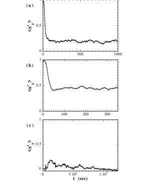
Figure 8: Tangle’s polarization $<s^{\prime}_{z}>$ vs time $t$ at $T=1.6{\rm K}$ and $V_{ns}=0.08{\rm cm/sec}$ for: (a): $\Omega=9.97\times 10^{-3}{\rm rad/sec}$; (b): $\Omega=4.98\times 10^{-2}{\rm rad/sec}$. (c): $\Omega=0{\rm rad/sec}$.

Figure 9 shows the calculated dependence of the vortex line density $L$ on the counterflow velocity $V_{ns}$ at different rotation rates $\Omega$. The figure shows a dependence of $L$ on $V_{ns}$ which is similar to what appears in the Fig. 1 of the paper by Swanson et al Swanson . The only difference is that the scale of the axes in the paper by Swanson al. is bigger - in this particular figure they report vortex line densities as high as $L\approx 2500\rm cm^{-2}$, whereas our calculations are limited to $L\approx 80\rm cm^{-2}$. Despite the lack of overlap between the experimental and numerical ranges, there is clear qualitative similarity between the figures. It is apparent that the critical velocity beyond which $L$ increases with $V_{ns}$ is much reduced by the presence of rotation, which is consistent with the observations.

Figure 10 shows the calculated polarization $<s^{\prime}_{z}>$ as a function of counterflow velocity $V_{ns}$ at different rotation rates $\Omega$. It is apparent that the polarization decreases with the counterflow velocity and increases with the rotation, which shows the competition between order induced by rotation and disorder induced by flow.

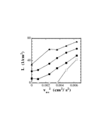
Figure 9: Vortex line density $L$ vs $V_{ns}^{2}$ at $T=1.6{\rm K}$ for $\Omega=0$ (white square), $\Omega=9.97\times 10^{-3}{\rm rad/sec}$ (black square), $\Omega=2.99\times 10^{-2}{\rm rad/sec}$ (circle) and $\Omega=4.98\times 10^{-2}{\rm rad/sec}$ (triangle). The dotted lines are guides to the eye.

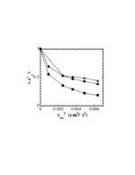
Figure 10: Tangle’s polarization $<s^{\prime}_{z}>$ vs $V_{ns}^{2}$ at $T=1.6{\rm K}$ for $\Omega=9.97\times 10^{-3}{\rm rad/sec}$ (square), $\Omega=2.99\times 10^{-2}{\rm rad/sec}$ (circle) and $\Omega=4.98\times 10^{-2}{\rm rad/sec}$ (triangle).The dotted lines are guides to the eye.

We conclude that the nonlinear saturation which takes place beyond the DG instability and which was observed by Swanson et al.Swanson is a state of ”polarized” turbulence.

VII The second critical velocity

In this section we propose a qualitative theory for the second critical velocity which was observed, but not explained, by Swanson et al. Swanson . Unfortunately, this region of parameter space cannot be explored directly using numerical methods, due to the larger vortex line densities.

We consider the following idealized model of the region $V_{ns}>V_{c2}$. We represent the polarized tangle as the combination of a vortex array and a number of vortex loops which are randomly oriented, so that the combined system is in balance and has the necessary amount of length and polarization. Let $\tau_{1}$ be the characteristic timescale of the growing Kelvin waves which are induced on the vortex array by the DG instability. The typical lifetime $\tau_{2}$ of the vortex loops will be determined by the friction with the normal fluid and by the relative orientation with respect to the counterflow. If $\tau_{2}>\tau_{1}$ then the vortex loops will not have enough time to shrink significantly before more loops are introduced by vortex reconnections induced by growing Kelvin waves. The combined system consisting of the vortex array and the vortex loops will not be balanced any longer because randomness is introduced by vortex reconnections at a rate which is faster than the rate at which loops are destroyed by friction. In conclusion, we expect that the vortex tangle will be turbulent and unpolarized. According to this scenario, the order of magnitude of the critical velocity $V_{c2}$ is given by the condition

$$\tau_{1}=\tau_{2}.$$ (17)

First we estimate $\tau_{1}$ using a simple model. For the sake of simplicity we assume an isolated vortex line of helical shape $\vec{s}=(\epsilon\cos{\phi};\epsilon\sin{\phi};z)$ where $\phi=kz-\omega t$ and $\epsilon<<1$, hence $z\approx\xi$ is the arc-length. The tangent unit vector is $\vec{s}^{\prime}=d{\vec{s}}/d\xi\approx d{\vec{s}}/dz=(-k\epsilon\sin{\phi};k\epsilon\cos{\phi};1)$ and ${\vec{s}}^{\prime\prime}=(-k^{2}\epsilon\cos{\phi};-k^{2}\epsilon\sin{\phi};0)$. Using the localized-induction approximation, the self-induced velocity of the line at the point ${\bf s}$ is given by

$$\vec{v}_{i}=\nu^{\prime}\vec{s}^{\prime}\times\vec{s}^{\prime\prime},$$ (18)

where $\nu^{\prime}=\kappa{\cal L}_{1}/(4\pi)$ and the slowly varying term ${\cal L}_{1}=\ln{[1/(ka_{0})]}$ is assumed constant. Neglecting higher order terms in $\epsilon$ we have $\vec{v}_{i}=\nu^{\prime}k^{2}\epsilon(\sin{\phi};-\cos{\phi};0)$.

In the absence of friction the equation of motion is simply $d{\vec{s}}/dt={\vec{v}}_{i}$, hence, assuming that $\epsilon$ is constant, we find that the Kelvin wave oscillates with angular frequency $\omega=\nu^{\prime}k^{2}$. This result differs from Glaberson’s Eq. (13) because we perturbed a single vortex line rather than a continuum of vorticity $2\Omega$ described by the Hall-Vinen equations in the rotating frame (hence the presence of a different upper cutoff which makes $\nu^{\prime}$ different from $\nu$ and the contribution $2\Omega$ to $\omega$).

In the presence of friction, neglecting the small mutual friction coefficient $\alpha^{\prime}$ for simplicity, the equation of motion is $d{\vec{s}}/dt=\vec{v}_{i}+\alpha\vec{s}^{\prime}\times(\vec{v}_{\rm ns}-\vec{v}_{i})$. Assuming $\vec{v}_{\rm ns}=(0;0;V_{ns})$ and $\epsilon=\epsilon(t)$, we find that $d\epsilon/dt=\alpha(kV_{ns}-\nu^{\prime}k^{2})\epsilon$ hence $\epsilon(t)=\epsilon(0)exp(\sigma t)$ where the growth rate is $\sigma=\alpha(kV_{ns}-\nu^{\prime}k^{2})$. Given $V_{ns}$, the largest growth rate occurs for $k=V_{ns}/(2\nu^{\prime})$ and takes $\sigma=\alpha V_{ns}^{2}/(4\nu^{\prime})$, for which we conclude that

$$\tau_{1}=\frac{1}{\sigma}=\frac{4\nu^{\prime}}{\alpha V_{ns}^{2}}.$$ (19)

To estimate $\tau_{2}$ we approximate the vortex loops as vortex rings of radius approximately determined by the average vortex spacing $\delta\approx L^{-1/2}$. The characteristic lifetime of a ring of radius $R$ in the presence of friction is BDV1

$$\tau_{2}=\frac{2\rho_{s}\pi R^{2}}{\gamma{\cal L}_{2}},$$ (20)

where ${\cal L}_{2}=\ln{[(8R/a_{0})-1/2]}$ and $\gamma$ is a known friction coefficient BDV1 . Setting $2R=\delta=L^{-1/2}$, we conclude that the polarized tangle is unstable if

$$L<C_{2}V_{ns}^{2},$$ (21)

with

$$C_{2}=\frac{\alpha\pi^{2}\rho_{s}}{2\gamma\Gamma{\cal L}_{1}{\cal L}_{2}}.$$ (22)

Equation  (21) has the same dependence of $L$ on $V_{ns}$ as that observed experimentally. At $T=1.65{\rm K}$ we have BDV1 $\rho_{s}=0.1168{\rm g/cm^{3}}$, $\gamma=1.3\times 10^{-5}{\rm g/cm~{}sec}$, $\alpha=0.11$. Since $a_{0}\approx 10^{-8}{\rm cm}$ and the slowly varying logarithm terms are approximately ${\cal L}_{1}\approx{\cal L}_{2}\approx 10$, we conclude that $C_{2}\approx 5\times 10^{4}{\rm cm^{-4}sec^{2}}$, which is of the same order of magnitude of the value $C_{2}=16\times 10^{4}{\rm cm^{-4}sec^{2}}$ found by Swanson et alSwanson .

VIII Conclusions

In conclusion, we have studied the stability of a superfluid vortex array in the presence of an applied counterflow, giving answers to some questions which were first asked by the pioneering experiment of Swanson et alSwanson . After investigating the DG instability, we have determined the existence of a new state of superfluid turbulence (polarized turbulence) which is characterized by two statistically steady state properties, the vortex line density and the degree of polarization. Although our computed range of vortex line densities does not overlap with the much higher values obtained in the experiment, we find the same qualitative dependence of vortex line density versus counterflow velocity at different rotations. We have also made some qualitative progress to understand what happens beyond $V_{c2}$.

Further work with more computing power will hopefully investigate other aspects of the problem, particularly what happens at high counterflow velocities and line densities. We also hope that our work will stimulate more experiments on this problem.

It is somewhat surprising that so little is known about the destabilization of a rotational vortex array by an imposed counterflow. For example, it should be possible to observe the polarization of turbulence by using simultaneous measurements of second sound attenuation along and across the rotation axis.

Finally, our work should be of interest to other investigations of vortex arrays and how they can be destabilized in other systems, ranging from superfluid ³He Helsinki to atomic Bose-Einstein condensates TKU . It is also worth noticing that this study has revealed the crossover of the dimensionality of vortex systems. If one considers the three regimes in Fig. 2 one notices that, at a fixed value of $V_{ns}$, increasing the rotation rate makes the vortices polarized, changing the dynamics from three-dimensional to two-dimensional. This reduction of the dimensionality of turbulence has been observed in classical fluid mechanics Hossain .

ACKNOWLEDGEMENTS

The authors thank W.F.Vinen for useful discussions. C.F.B. is grateful to the Royal Society for financially supporting this project. M.T. is grateful to Japan Society for the Promotion of Science for financially supporting this Japan-UK Scientific Cooperative Program(Joint Research Project).

References

- (1) R.J. Donnelly, Quantized Vortices In Helium II, Cambridge University Press, Cambridge (1991).
- (2) C.F. Barenghi, R.J. Donnelly and W.F. Vinen. Quantized Vortex Dynamics And Superfluid Turbulence, Springer’s Lecture Notes in Physics 571 (2001).
- (3) A.L. Fetter, Phys. Rev. 152 183 (1966).
- (4) D. K. Cheng, M.W. Cromar and R.J. Donnelly, Phys. Rev. Lett. 31, 433 (1973).
- (5) W.I. Glaberson, W.W. Johnson and R.M. Ostermeier, Phys. Rev. Lett. 33, 1197 (1974); R.M. Ostermeier and W.I. Glaberson, J. Low Temp. Phys. 21, 191 (1975).
- (6) D.C. Samuels and D. Kivotides, Phys. Rev. Lett. 83, 5306 (1999).
- (7) S.R. Stalp, L. Skrbek and R.J. Donnelly, Phys. Rev. Lett. 82, 4831 (1999).
- (8) J. Maurer and P. Tabeling, Europhys. Lett. 43, 29 (1998).
- (9) S.I.Davis, P.C. Hendry and P.V.E. McClintock, Physica 280B 43 (2000).
- (10) S.N. Fisher, A.J. Hale, A.M. Guenault and G.R. Pickett, Phys. Rev. Lett. 86 244 (2001).
- (11) C.F. Barenghi, G.G. Bauer, D.C. Samuels and R.J. Donnelly, Phys. Fluids 9, 2631 (1997).
- (12) C.F. Barenghi, S. Hulton and D.C. Samuels, Phys. Rev. Lett. 89 275301 (2002).
- (13) T. Araki, M. Tsubota and S.K. Nemirovskii, Phys. Rev. Lett. 89, 145301 (2002).
- (14) W.F. Vinen, Phys. Rev. B 61, 1410 (2000); W.F. Vinen & J.J. Niemela, J. Low Temp. Phys. 129, 213 (2002).
- (15) C.E. Swanson, C.F. Barenghi and R.J. Donnelly, Phys. Rev. Lett. 50 190 (1983).
- (16) K.W. Schwarz, Phys. Rev. B 31, 5782 (1985); Phys. Rev. B 38, 2398 (1988).
- (17) J.T. Tough, in Progress in Low Temperature Physics, edited by D.F. Brewer, North-Holland (Amsterdam), 8 (1981).
- (18) W.F.Vinen, Proc. R. Soc. London, Ser. A242, 493(1957); Ser. A243, 400(1958).
- (19) D.J. Melotte and C.F. Barenghi, Phys. Rev. Lett. 80, 4181 (1998).
- (20) C.F. Barenghi, K. Park and R.J. Donnelly, Phys. Lett. A84, 453 (1981).
- (21) M. Tsubota, T. Araki and S.K. Nemirovskii, Phys. Rev. B 62 11751 (2000).
- (22) M. Tsubota and H. Yoneda, J. Low Temp. Phys. 101 815 (1995).
- (23) L.M. Milne-Thomson, Theoretical Hydrodynamics 5th Edition, Macmillan, London(1968).
- (24) J. Koplik and H. Levine, Phys. Rev. Lett. 71, 1375 (1993).
- (25) P.G. Drazin and W.H. Reid, Hydrodynamics Stability, Cambridge University Press, Cambridge (1981).
- (26) M. Tsubota, T. Araki and C.F. Barenghi, Phys. Rev. Lett. 90, 205301 (2003).
- (27) C.F. Barenghi, R.J. Donnelly and W.F. Vinen, J. Low Temp. Phys. 52, 189(1983).
- (28) R.T. Wang, C.E. Swanson and R.J. Donnelly, Phys. Rev. B 36, 5240 (1987).
- (29) A.P.Finne, T. Araki, R. Blaauwgeers, V.B. Eltsov, N.B. Kopnin, M. Krusius, L. Skrbek, M. Tsubota, and G.E. Volovik, cond-mat/0304586.
- (30) M. Tsubota, K. Kasamatsu and M. Ueda, Phys. Rev. A 65, 023603 (2002).
- (31) M. Hossain, Phys. Fluids 6, 1077 (1994).