Strong coupling approach in dynamical mean-field theory for strongly correlated electron systems

Abstract

We review two analytical approaches in Dynamical Mean-Field Theory (DMFT) based on a perturbation theory expansion over the electron hopping to and from the self consistent environment. In the first approach the effective single impurity Anderson model (SIAM) is formulated in terms of the auxiliary Fermi-fields and the projection (irreducible Green’s function) technique is used for its solution. A system of the DMFT equations is obtained that includes as simple specific cases a number of known approximations (Hubbard-III, AA, MAA, …). The second approach is based on the diagrammatic technique (Wick’s theorem) for Hubbard operators that allows to construct a thermodynamically consistent theory when SIAM exactly splits into four components (subspaces): two Fermi liquid and two non-Fermi liquid. The results for the density of states, concentration dependences of the band energies, chemical potential and magnetic order parameters are presented for different self-consistent approximations (AA, strong coupling Hartree–Fock and further).

1 Introduction

Many unconventional properties (e.g., metal–insulator transition, electronic (anti)ferromagnetism) of the narrow-band systems (transition metals and their compounds, some organic systems, high-$T_{c}$ superconductors, etc.) can be explained only by the proper treatment of the strong local electron correlations. The simplest models allowing for the electron correlations are a single-band Hubbard model with on-site repulsion $U$ and hopping energy $t$ and its strong-coupling limit ($U\gg t$): $t-J$ model. Recent studies of the Hubbard-type models connected mainly with the theory of high-$T_{c}$ superconductivity and performed in the weak- $(U\leq 4t)$ and strong- $(U\gg t)$ coupling limits, elucidate some important features of these models [1]. But still a lot of problems remains, especially for the $U\gg t$ case where there are no rigorous approaches.

Despite the relative simplicity of the models used for their description the theory of electron spectrum and thermodynamic properties of such systems is far from its final completion. The use of localized (atomic) basis of electron states is the general feature of the models. Corresponding Hamiltonians

$$H=\sum_{i}H_{i}+\sum_{\langle ij\rangle}\sum_{\sigma}t_{ij}a_{i\sigma}^{\dagger}a_{j\sigma}$$ (1)

include, on the one hand the electron transfer (hopping) $t_{ij}$ between neighbouring sites (atoms) in the crystal lattice and on the other hand the short-range single-site electron correlations. It is primarily the on-site energy of Coulomb repulsion $U$ in the case of the Hubbard model and the models based on that one:

$$H_{i}=Un_{i\uparrow}n_{i\downarrow}-\mu\sum_{\sigma}n_{i\sigma}\;.$$ (2)

Models like (1), (2) can be solved exactly in two limiting cases: atomic limit ($t=0$) and band electrons ($U=0$). Near these extreme cases the expansions in terms of $t$ or $U$ are used, but the consistent formulation of the perturbation theory especially in the case of strong coupling is not a simple task. The case of an intermediate coupling $t\sim U$ is more complicated for consideration. In this region of parameter values, the splitting in the band electron spectrum and the metal–insulator transition takes place.

Due to the presence of strong electron correlations, the state of the electron system and its properties depend essentially on the mean electron concentration. At a different filling of electron states and depending on the relation between $t$ and $U$ parameters, the system can be paramagnetic or the transition into ferro- (antiferro-) magnetic phase can take place. In the case of the more complicated structure of the Hamiltonian $H_{i}$ (due to the allowance for the other, besides electron, degrees of freedom) or when the interaction is extended to the nearest neighbours in a lattice, the charge ordering can appear; the effects of phase separation become possible as well. The listed phenomena are the subject of study in the framework of various approaches and methods.

A new impulse in the investigations in this field is connected with the development of a new approach having its origin in works [2, 3, 4] where the study of the (1), (2)-type model in the limit of infinite dimensionality of space ($d=\infty$) has been proposed. Due to the principal simplifications in the perturbation series taking place in this case the possibility exists to obtain exact results using the scheme that corresponds to the well known coherent potential approximation (CPA) in the theory of disordered crystalline alloys. The rapidly developing corresponding method became known as the dynamical mean-field theory (DMFT).

The central point in this method is formulation and solution of the auxiliary single-site problem. An initial model is mapped on that one while considering one site characteristics of the electron spectrum, such as single-site electron Green’s function (see [5, 6, 7], as well as the reviews [8, 9]). In this case the separated lattice site is considered as placed in some effective environment. Since the processes of electron hopping from the atom and returning into the atom are taken into account, the mean field acting on the electron states of the atom possesses a dynamical nature. This field is described by the coherent potential $J_{\sigma}(\omega)$ that should be determined in a self-consistent way. The analytical properties of the solutions in the DMFT are considered in [10].

Only in some simple cases the single-site problem can be solved analytically [11, 12] (e.g., the Falicov–Kimball (FK) model [13]). In general, including the Hubbard model, the application of numerical or seminumerical (such as quantum Monte Carlo [6, 14, 15] or exact diagonalization [16, 17] as well as numerical renormalization group [18], see [9]) methods turns out to be necessary.

At present, the Dynamical Mean-Field Theory is applied to investigate different effects in the various systems described by the simplified or realistic models. First applications were devoted to the investigation of the changes of the density of states at the metal-insulator transition and appearance of the antiferromagnetic and ferromagnetic states in the Hubbard model [6, 15, 19, 20, 21, 22, 23, 24, 25, 26, 27, 28, 29] and other strongly correlated electron models: Hubbard model with orbiral degeneracy [30] and disorder [31], boson-fermion model [32], extended Hubbard model [33], double-exchange model [34], Falicov–Kimball model with correlated hopping [35], two-band Hubbard model [36, 37], periodic Anderson model [38].

Besides, different types of the response functions and transport coefficients are also calculated. The general basics how to derive response functions in DMFT are given in [11, 39, 12]. Investigations of the charge and magnetic susceptibilities revealed also chess-board charge-density-wave phase at half-filling [11] as well as incommensurate order and phase separation at other fillings [40, 41]. DMFT is used also to investigate optical conductivity [20, 21, 42, 43], electronic Raman scattering [44, 45], thermoelectric response [46].

In last years, DMFT is used as an approximation scheme to consider the electron-electron interaction together with band degeneracy and lattice structure of the actual materials within the so-called LDA+DMFT approach, that allows to describe correctly the insulating state of the transition-metal oxides, band structure and phase diagrams of the different compounds [47, 48].

At the same time it is of interest to develop approximate analytic approaches to the solution of the single-site problem. Their application at that stage is more effective than at considering the full model (a short review of such attempts was given recently in [51, 52]). The availability of the analytical (even of approximate) method is useful especially for new models as well as at the transition to the finite dimensionality of the system. The accuracy of approximation can be estimated relating to the results of numerical calculations.

The first analytical approximation proposed for the Hubbard model was a simple Hubbard-I approximation [53] (see Ref. [54] for its possible improvement) which is correct in the atomic ($t=0$) and band ($U=0$) limits but is inconsistent in the intermediate cases and cannot describe the metal–insulator transition. Hubbard’s alloy-analogy solution [55] (so-called Hubbard-III approximation) incorporates into the theory an electron scattering on the charge and spin fluctuations that allows us to give qualitative description of the changes of the density-of-state at the metal–insulator transition point. Hubbard-I and Hubbard-III approximations introduce two types of particles (electrons moving between empty sites and electrons moving between sites occupied by electrons of opposite spin) with the different energies that differ by $U$ and form two Hubbard bands. Related schemes of the so-called two-pole approximations [56, 57], which are justified by the $t/U\ll 1$ perturbation theory expansions [58], are also considered. However, in the recent QMC studies [59, 60] there are clearly distinguished four bands in the spectral functions rather than the two bands predicted by the two-pole approximations. Such four-band structure is reproduced by the strong-coupling expansion for the Hubbard model [60] in the one-dimensional case. There are also analytical approximations developed specially for the effective environment in the DMFT [49, 50]. Within other approaches let us mention non-crossing approximation [21, 61], Edwards–Hertz approach [62, 63], iterative perturbation theory [64, 65], alloy-analogy based approaches [66, 67], and linked cluster expansions [4, 68], which are reliable in certain limits and the construction of the thermodynamically consistent theory still remains open [52].

The aim of this paper is to review two recently proposed approaches [69, 70] based on the rigorous perturbation theory scheme in terms of electron hopping for the Hubbard-type models.

The first approach [69] is based on the technique of the irreducible Green’s functions. The procedure of projecting onto the basic set of operators is used (the set consists of the single-site electron Hubbard operators of the Fermi-type). The recipe is given for the construction of the system of equations for the coherent potential and self-consistency parameter (having the meaning of a static part of the effective internal field) in the approach that is a generalization of the Hubbard-III approximation. Specific cases are considered corresponding to the more simple approximations of the alloy-analogy (AA) or modified alloy-analogy (MAA) type [52, 66] in the DMFT method as well as to the certain decoupling procedure in the two-time Green’s function method when applied to the initial electron problem.

Another possibility is to build analytical approaches by the systematic perturbation expansion in terms of the electron hopping [71, 72, 73] using diagrammatic technique for Hubbard operators [74, 75]. One of them was proposed for the Hubbard ($U=\infty$ limit) and $t-J$ models [76, 77]. The lack of such approach is connected with the concept of a ‘‘hierarchy’’ system for Hubbard operators when the form of the diagrammatic series and final results strongly depend on the system of the pairing priority for Hubbard operators. On the other hand it is difficult to generalize it on the case of the arbitrary $U$.

In the second part of this paper we show how a rigorous perturbation theory scheme in terms of electron hopping that is based on the Wick’s theorem for Hubbard operators [74, 75] and is valid for arbitrary value of $U$ ($U<\infty$) and does not depend on the ‘‘hierarchy’’ system for $X$ operators can be developed for the Hubbard-type models [70]. In the limit of infinite spatial dimensions, these analytical schemes allow us to build a self-consistent Baym–Kadanoff type theory [78, 79] for the Hubbard model and some analytical results are given for simple approximations. The Falicov–Kimball model is also considered as an exactly solvable limit of Hubbard model.

2 Hubbard model and similar models in a limit of infinite dimension of space ($d=\infty$)

The transition to the $d=\infty$ limit in the DMFT approach is accompanied by the scaling of the electron transfer parameter

$$t=\frac{t^{*}}{\sqrt{d}}\;.$$ (3)

In the case of $d$-dimensional hypercubic lattice with an electron spectrum

$$\varepsilon_{k}=\frac{2t^{*}}{\sqrt{d}}\sum_{\alpha=1}^{d}\cos k_{\alpha}a\;,$$ (4)

this procedure leads to the Gaussian density of electron states [2]

$$\rho_{0}(\omega)=\frac{1}{2\sqrt{\pi}t^{*}}\exp\left(-\frac{\omega^{2}}{4t^{*2}}\right)\;.$$ (5)

The average kinetic energy remains constant in this case in the limit $d=\infty$.

The scaling (3) has a significant effect on the structure of diagrammatic series for single-electron Green’s functions of the model of the (1) and (2) type. In particular, the irreducible self-energy part of such a function becomes a purely local (a single-site) quantity [2, 3]:

$$\Sigma_{ij,\sigma}(\omega)=\Sigma_{\sigma}(\omega)\delta_{ij}\;,\qquad d=\infty\;.$$ (6)

The Fourier-transform of $\Sigma_{ij,\sigma}(\omega)$ is hence momentum-independent

$$\Sigma_{\sigma}(\mathbf{k},\omega)=\Sigma_{\sigma}(\omega)\;.$$ (7)

This leads to tremendous simplifications in all many-body calculations for the Hubbard model and related models and enables us to obtain the exact numerical results for the main parameters of the electron spectrum, to describe magnetic phase transitions and the metal–insulator transformation etc. (see, for example, [9, 52]).

The possibility of obtaining exact solutions in the $d=\infty$ limit opens the way to the development of a theory based on the expansion in powers of $1/d$ (the results for $d=\infty$ can be considered as zero approximation in this case). Such approaches have been elaborated for the last few years [80, 81]. On the other hand, consideration in the framework in the $d=\infty$ limit is not only of an academic interest. It turns out that a set of the known approximating schemes or methods is correct in the $d=\infty$ limit. Besides, the obtained physical conclusions can be transferred in many cases to the system with finite dimensions keeping their suitability even at $d=3$.

The formal scheme of calculating the electron Green’s functions and the main thermodynamical quantities can be developed basing on the diagrammatic expansions in powers of interaction parameters (such as energy $U$ in the case of the Hubbard model) or matrix elements of the electron transfer $t_{ij}$. The electron Green’s function in ($\mathbf{k},\omega$) representation

$$G_{k}^{\sigma}(\omega)=\sum_{i-j}\mathrm{e}^{\mathrm{i}\mathbf{k}(\mathbf{R}_{i}-\mathbf{R}_{j})}G_{ij,\sigma}(\omega)$$ (8)

can be expressed in the first or in the second of these cases as

$$G_{\mathbf{k}}^{\sigma}(\omega)=\frac{1}{\omega+\mu-t_{\mathbf{k}}-\Sigma_{\sigma}(\omega)}$$ (9)

or

$$G_{\mathbf{k}}^{\sigma}(\omega)=\frac{1}{\Xi_{\sigma}^{-1}(\omega)-t_{\mathbf{k}}}\;,$$ (10)

where $\Sigma_{\sigma}(\omega)$ or $\Xi_{\sigma}(\omega)$ are the irreducible parts (in the diagrammatic representation) according to Dyson or Larkin, respectively,

$$\Xi_{\sigma}^{-1}(\omega)=\omega+\mu-\Sigma_{\sigma}(\omega)\;.$$ (11)

To calculate the $\Sigma_{\sigma}(\omega)$ [or $\Xi_{\sigma}(\omega)$] function, the effective single-site problem is used. As was shown in [11], the transition to this problem corresponds to the replacement

$$\mathrm{e}^{-\beta H}\to\mathrm{e}^{-\beta H_{\mathrm{eff}}}=\mathrm{e}^{-\beta H_{0}}$$ (12)

$$\times T\exp\left\{\!{-}\int_{0}^{\beta}\!\!\!\mathrm{d}\tau\int_{0}^{\beta}\!\!\!\mathrm{d}\tau^{\prime}\sum_{\sigma}J_{\sigma}(\tau{-}\tau^{\prime})a_{\sigma}^{\dagger}(\tau)a_{\sigma}(\tau^{\prime})\right\},$$

where

$$H_{0}=H_{i}$$ (13)

and $J_{\sigma}(\tau-\tau^{\prime})$ is an effective auxiliary field which is determined self-consistently from the condition that the same irreducible part $\Xi_{\sigma}(\omega)$ determines the lattice function (10) as well as the Green’s function $G_{\sigma}^{(a)}(\omega)$ of the effective single-site problem. The last one is connected with $\Xi_{\sigma}(\omega)$ and $J_{\sigma}(\omega)$ by the relation

$$G_{\sigma}^{(a)}(\omega)=\frac{1}{\Xi_{\sigma}^{-1}(\omega)-J_{\sigma}(\omega)}\;.$$ (14)

On the other hand,

$$G_{\sigma}^{(a)}(\omega)=G_{ii,\sigma}(\omega)=\frac{1}{N}\sum_{\mathbf{k}}G_{\mathbf{k}}^{\sigma}(\omega)\;.$$ (15)

Dynamical field $J_{\sigma}(\tau-\tau^{\prime})$ describes electron hopping from the given site into the environment and vice versa; the electron propagates in the environment without going through this site between moments $\tau$ and $\tau^{\prime}$. The expression

$$J_{\sigma}(\omega)=\sum_{kj}t_{ik}t_{ij}G_{kj,\sigma}^{(i)}$$ (16)

corresponds to this situation (the relation (16) is known from the standard CPA scheme [82, 83]); here $G_{kj,\sigma}^{(i)}$ is the electron Green’s function for a crystal with the removed site $i$.

The set of equations (10), (14) and (15) becomes closed when it is supplemented by the functional dependence

$$G_{\sigma}^{(a)}(\omega)=f([J_{\sigma}(\omega)])\;,$$ (17)

which is obtained as the result of solving the effective single-site problem with the statistical operator $\exp(-\beta H_{\mathrm{eff}})$. It is possible to do this in an analytical way only in some cases of simple models (a Falicov–Kimball model [11]; a pseudospin–electron model at $U=0$ [84]; a usual binary alloy model). In general, numerical methods are used.

The scheme described lies at the basis of the above mentioned DMFT approach used in the last years in considering strongly correlated electron systems.

3 Electron Green’s functions of the effective single-site problem

As it was mentioned, the central point in the DMFT approach is the solution of the effective single-site problem and the determination of the connection between the dynamical mean field (coherent potential) $J_{\sigma}(\omega)$ and the single-site electron Green’s function $G_{\sigma}^{(a)}(\omega)$. Recently an approximate scheme [69], which is based on the technique of the irreducible two-time temperature Green’s functions and leads to the results having an interpolating character, was proposed. The Hubbard model is taken into consideration to illustrate the method.

Let us reformulate a single-site problem introducing explicitly an effective Hamiltonian

$$\tilde{H}_{\mathrm{eff}}=H_{0}+V\sum_{\sigma}(a_{\sigma}^{\dagger}\xi_{\sigma}+\xi_{\sigma}^{\dagger}a_{\sigma})+H_{\xi}\;,$$ (18)

where the auxiliary Fermi-field $(\xi_{\sigma},\xi_{\sigma}^{\dagger})$ is brought in. It describes the environment of the selected site and formally is characterized by the Hamiltonian $H_{\xi}$. The single-electron transitions between the site and the environment are taken into account.

An explicit form of the Hamiltonian $H_{\xi}$ is unknown. Let us consider, however, the Green’s function

$${\cal{G}}_{\sigma}(\omega)=\langle\langle\xi_{\sigma}|\xi_{\sigma}^{\dagger}\rangle\rangle_{\omega}^{(H_{\xi})}$$ (19)

for auxiliary fermions as the given function. The Green’s function ${\cal{G}}_{\sigma}(\tau{-}\tau^{\prime})=\langle T_{\tau}\xi_{\sigma}^{\dagger}(\tau)\xi_{\sigma}(\tau^{\prime})\rangle_{\xi}$ [where averaging is performed with the part $H_{\xi}$ of the Hamiltonian (18)] corresponds to the function (19) in the Matsubara’s representation. It is shown in [69] that the expansion of the $\exp(-\beta\tilde{H}_{\mathrm{eff}})$ operator in powers of $V$ and the subsequent averaging over the states of $\xi$-subsystem using the Wick’s theorem and functions (19) leads to the statistical operator (12):

$$\langle\exp(-\beta\tilde{H}_{\mathrm{eff}})\rangle^{(H_{\xi})}=\exp(-\beta H_{\mathrm{eff}})\;.$$ (20)

The relation

$$2\pi V^{2}{\cal{G}}_{\sigma}(\omega)=J_{\sigma}(\omega)$$ (21)

takes place in this case.

The obtained result points out to the possibility of the Green’s function $G_{\sigma}^{(a)}(\omega)$ calculation based on the Hamiltonian $\tilde{H}_{\mathrm{eff}}$. The averaging over the $a$, $a^{\dagger}$-variables is performed with the use of the Gibbs distribution while over the $\xi$, $\xi^{\dagger}$-variables it is done with the help of function (19).

Let us write the Hamiltonian (18) for the case of the Hubbard model in terms of Hubbard operators

$$\tilde{H}_{\mathrm{eff}}=-\mu\biggl{(}\sum\limits_{\sigma}X^{\sigma\sigma}+2X^{22}\biggr{)}+UX^{22}+$$

$$\quad+V\sum\limits_{\sigma}\left[(X^{\sigma 0}+\sigma X^{2\bar{\sigma}})\xi_{\sigma}+\xi_{\sigma}^{\dagger}(X^{0\sigma}+\sigma X^{\bar{\sigma}2})\right]+$$

$$\quad+H_{\xi}\;.$$ (22)

Here the basis of single-site states $|n_{\uparrow}n_{\downarrow}\rangle$

$$\begin{array}[]{ll}|0\rangle=|0,0\rangle\;,&|\downarrow\rangle=|0,1\rangle\;,\\ |2\rangle=|1,1\rangle\;,&|\uparrow\rangle=|1,0\rangle\end{array}$$ (23)

is used ($\sigma=\uparrow,\downarrow$). In this case the Green’s function $G_{\sigma}^{(a)}(\omega)$ can be written in the form

$$G_{\sigma}^{(a)} = \langle\langle X^{0\sigma}|X^{\sigma 0}\rangle\rangle_{\omega}{+}\sigma\langle\langle X^{0\sigma}|X^{2\bar{\sigma}}\rangle\rangle_{\omega}$$ (24)

$$+ \sigma\langle\langle X^{\bar{\sigma}2}|X^{\sigma 0}\rangle\rangle_{\omega}{+}\langle\langle X^{\bar{\sigma}2}|X^{2\bar{\sigma}}\rangle\rangle_{\omega}$$

(a representation in terms of the two-time Green’s functions is used).

We will write the equations for functions (24) using the equations of motion for $X$-operators:

$$\mathrm{i}\frac{\mathrm{d}}{\mathrm{d}t}X^{0\sigma}(t) = [X^{0\sigma},\tilde{H}_{\mathrm{eff}}]=-\mu X^{0\sigma}+V(X^{00}+X^{\sigma\sigma})\xi_{\sigma}$$

$$+ VX^{\bar{\sigma}\sigma}\xi_{\bar{\sigma}}+\sigma VX^{02}\xi_{\bar{\sigma}}^{\dagger}\;,$$

$$\mathrm{i}\frac{\mathrm{d}}{\mathrm{d}t}X^{\bar{\sigma}2}(t) = [X^{\bar{\sigma}2},\tilde{H}_{\mathrm{eff}}]=(U-\mu)X^{\bar{\sigma}2}$$

$$+ \sigma V(X^{22}+X^{\bar{\sigma}\bar{\sigma}})\xi_{\sigma}{-}\sigma VX^{\bar{\sigma}\sigma}\xi_{\bar{\sigma}}{-}VX^{02}\xi_{\bar{\sigma}}^{\dagger}\;.$$

In the Green’s functions of higher order we shall separate the irreducible parts using the method developed in [85, 86]. Proceeding from the equations of motion (3) we express derivatives $\mathrm{i}\,\mathrm{d}X^{0\sigma(\bar{\sigma}2)}/\mathrm{d}t$ as a sum of regular (projected on the subspace formed by operators $X^{0\sigma}$, $X^{\bar{\sigma}2}$) and irregular parts. The latter ones describe an inelastic quasiparticle scattering. We obtain

$$[X^{0\sigma},\tilde{H}_{\mathrm{eff}}] = -\mu X^{0\sigma}+\alpha_{1}^{0\sigma}X^{0\sigma}+\alpha_{2}^{0\sigma}X^{\bar{\sigma}2}+Z^{0\sigma}\;,$$

$${}[X^{\bar{\sigma}2},\tilde{H}_{\mathrm{eff}}] = (U-\mu)X^{\bar{\sigma}2}+\alpha_{1}^{\bar{\sigma}2}X^{0\sigma}$$ (26)

$$+ \alpha_{2}^{\bar{\sigma}2}X^{\bar{\sigma}2}+Z^{\bar{\sigma}2}\;.$$

Operators $Z^{0\sigma}$ and $Z^{\bar{\sigma}2}$ are defined as orthogonal ones to operators from the basic subspace:

$$\langle\{Z^{0\sigma(\bar{\sigma}2)},X^{\sigma 0}\}\rangle = 0\;,$$

$$\langle\{Z^{0\sigma(\bar{\sigma}2)},X^{2\bar{\sigma}}\}\rangle = 0\;.$$ (27)

These equations determine the coefficients $\alpha_{i}^{0\sigma(\bar{\sigma}2)}$.

Using the described procedure we come to the expressions

$$Z^{0\sigma} = V\overline{(X^{00}+X^{\sigma\sigma})\xi_{\sigma}}+V\overline{X^{\bar{\sigma}\sigma}\xi_{\bar{\sigma}}}+\sigma V\overline{X^{02}\xi_{\bar{\sigma}}^{\dagger}}\;,$$

$$Z^{\bar{\sigma}2} = \sigma V\overline{(X^{22}+X^{\bar{\sigma}\bar{\sigma}})\xi_{\sigma}}-\sigma V\overline{X^{\bar{\sigma}\sigma}\xi_{\bar{\sigma}}}$$ (28)

$$- V\overline{X^{02}\xi_{\bar{\sigma}}^{\dagger}}\;,$$

where

$$\overline{(X^{00}+X^{\sigma\sigma})\xi_{\sigma}}=(X^{00}+X^{\sigma\sigma})\xi_{\sigma}\;,$$

$$\overline{(X^{22}+X^{\bar{\sigma}\bar{\sigma}})\xi_{\sigma}}=(X^{22}+X^{\bar{\sigma}\bar{\sigma}})\xi_{\sigma}\;,$$

$$\overline{X^{\bar{\sigma}\sigma}\xi_{\bar{\sigma}}}=X^{\bar{\sigma}\sigma}\xi_{\bar{\sigma}}-\frac{1}{A_{0\sigma}}\langle\xi_{\bar{\sigma}}X^{\bar{\sigma}0}\rangle X^{0\sigma}$$

$$\qquad\quad-\frac{1}{A_{2\bar{\sigma}}}\langle X^{2\sigma}\xi_{\bar{\sigma}}\rangle X^{\bar{\sigma}2}\;,$$

$$\overline{X^{02}\xi_{\bar{\sigma}}^{\dagger}}=X^{02}\xi_{\bar{\sigma}}^{\dagger}-\frac{1}{A_{0\sigma}}\langle X^{\sigma 2}\xi_{\bar{\sigma}}^{\dagger}\rangle X^{0\sigma}$$

$$\qquad\quad-\frac{1}{A_{2\bar{\sigma}}}\langle\xi_{\bar{\sigma}}^{\dagger}X^{0\bar{\sigma}}\rangle X^{\bar{\sigma}2}$$ (29)

and $A_{pq}=\langle X^{pp}+X^{qq}\rangle$; $A_{0\sigma}=1-n_{\bar{\sigma}}$, $A_{\bar{\sigma}2}=n_{\bar{\sigma}}$.

Here

$$\alpha_{1}^{0\sigma} = -\sigma\alpha_{1}^{\bar{\sigma}2}=\frac{V}{A_{0\sigma}}\varphi_{\sigma}\;,$$

$$\alpha_{2}^{0\sigma} = -\sigma\alpha_{2}^{\bar{\sigma}2}=-\frac{V}{A_{2\bar{\sigma}}}\sigma\varphi_{\sigma}\;,$$

$$\varphi_{\sigma} = \langle\xi_{\bar{\sigma}}X^{\bar{\sigma}0}\rangle+\sigma\langle X^{\sigma 2}\xi_{\bar{\sigma}}^{\dagger}\rangle\;.$$ (30)

(we put $\varphi_{\sigma}=\varphi_{\sigma}^{*}$).

The equations for the first two functions in (24) have in this case the form

$$\left(\begin{array}[]{cc}\omega-a_{\sigma}&\sigma\frac{V}{A_{2\bar{\sigma}}}\varphi_{\sigma}\\ \sigma\frac{V}{A_{0\sigma}}\varphi_{\sigma}&\omega-b_{\sigma}\end{array}\right)\left(\begin{array}[]{c}\langle\langle X^{0\sigma}|X^{\sigma 0}\rangle\rangle\\ \langle\langle X^{\bar{\sigma}2}|X^{\sigma 0}\rangle\rangle\end{array}\right)$$ (35)

$$\qquad\qquad\qquad=\left(\begin{array}[]{c}\frac{A_{0\sigma}}{2\pi}+\langle\langle Z^{0\sigma}|X^{\sigma 0}\rangle\rangle\\ \langle\langle Z^{\bar{\sigma}2}|X^{\sigma 0}\rangle\rangle\end{array}\right)\;,$$ (38)

where the notations

$$a_{\sigma}=-\mu+\frac{V}{A_{0\sigma}}\varphi_{\sigma}\;,\qquad b_{\sigma}=U-\mu+\frac{V}{A_{2\bar{\sigma}}}\varphi_{\sigma}$$ (39)

are used (a similar set of equations can be written for functions $\langle\langle Z^{0\sigma(\bar{\sigma}2)}|X^{2\bar{\sigma}}\rangle\rangle$).

An equation for the Green’s function $\langle\langle Z^{0\sigma(\bar{\sigma}2)}|X^{\sigma 0}\rangle\rangle$ (as well as for the function $\langle\langle Z^{0\sigma(\bar{\sigma}2)}|X^{2\bar{\sigma}}\rangle\rangle$) can be obtained by means of the differentiation with respect to the second time argument. Applying the similar procedure of separation of the irregular parts we obtain the expression

$$\hat{G}=\hat{G}_{0}+\hat{G}_{0}\hat{P}_{\sigma}\hat{G}_{0}\;,$$ (40)

where the matrix Green’s function

$$\hat{G}=2\pi\left(\begin{array}[]{cc}\langle\langle X^{0\sigma}|X^{\sigma 0}\rangle\rangle&\langle\langle X^{0\sigma}|X^{2\bar{\sigma}}\rangle\rangle\\ \langle\langle X^{\bar{\sigma}2}|X^{\sigma 0}\rangle\rangle&\langle\langle X^{\bar{\sigma}2}|X^{2\bar{\sigma}}\rangle\rangle\end{array}\right)$$ (41)

is introduced. $\hat{G}_{0}$ is a nonperturbed Green’s function

$$\hat{G}_{0}=\frac{1}{D_{\sigma}}\left(\begin{array}[]{cc}\omega-b_{\sigma}&-\sigma\frac{V}{A_{2\bar{\sigma}}}\varphi_{\sigma}\\ -\sigma\frac{V}{A_{0\sigma}}\varphi_{\sigma}&\omega-a_{\sigma}\end{array}\right)\left(\begin{array}[]{cc}A_{0\sigma}&0\\ 0&A_{2\bar{\sigma}}\end{array}\right)\;,$$ (42)

where

$$D_{\sigma}=(\omega-a_{\sigma})(\omega-b_{\sigma})-\frac{V^{2}}{A_{0\sigma}A_{2\bar{\sigma}}}\varphi_{\sigma}^{2}$$ (43)

and

$$\hat{P}_{\sigma} = 2\pi\left(\begin{array}[]{cc}A_{0\sigma}^{-1}&0\\ 0&A_{2\bar{\sigma}}^{-1}\end{array}\right)\left(\begin{array}[]{cc}\langle\langle Z^{0\sigma}|Z^{\sigma 0}\rangle\rangle&\langle\langle Z^{0\sigma}|Z^{2\bar{\sigma}}\rangle\rangle\\ \langle\langle Z^{\bar{\sigma}2}|Z^{\sigma 0}\rangle\rangle&\langle\langle Z^{\bar{\sigma}2}|Z^{2\bar{\sigma}}\rangle\rangle\end{array}\right)$$ (48)

$$\times \left(\begin{array}[]{cc}A_{0\sigma}^{-1}&0\\ 0&A_{2\bar{\sigma}}^{-1}\end{array}\right)$$ (51)

has the meaning of a scattering matrix. Being expressed in terms of irreducible Green’s functions it contains the scattering corrections of the second and higher order in powers of $V$. The separation in $\hat{P}$ of the irreducible, with respect to $V$, parts enables us to obtain a mass operator $\hat{M}$

$$\hat{P}_{\sigma} = \hat{M}_{\sigma}+\hat{M}_{\sigma}\hat{G}_{0}\hat{M}_{\sigma}+\hat{M}_{\sigma}\hat{G}_{0}\hat{M}_{\sigma}\hat{G}_{0}\hat{M}_{\sigma}+\ldots\,,$$

$$\hat{M}_{\sigma} = \hat{P}_{\sigma}|_{\mathrm{ir}}\;.$$ (52)

In this case the relation (40) can be transformed into the Dyson equation

$$\hat{G}=\hat{G}_{0}+\hat{G}_{0}\hat{M}_{\sigma}\hat{G}$$ (53)

with the solution

$$\hat{G}=(1-\hat{G}_{0}\hat{M}_{\sigma})^{-1}\hat{G}_{0}\;,$$ (54)

which provides a final expression for the Green’s function (41).

4 Different-time decoupling of irreducible Green’s functions

We will restrict ourselves hereafter to the simple approximation in calculating the mass operator $\hat{P}$, taking into account the scattering processes of the second order in $V$. In this case

$$\hat{M}_{\sigma}=\hat{P}_{\sigma}^{(0)}\;,$$ (55)

where the irreducible Green’s functions are calculated without allowance for correlation between electron transitions on the given site and environment. It corresponds to the procedure of the different-time decoupling [87], which means in our case an independent averaging of the products of $X$ and $\xi$ operators.

Let us illustrate this approximation with some examples.

1. The Green’s function
$\langle\langle\overline{\vphantom{\xi_{\sigma}^{\dagger}}(X^{00}+X^{\sigma\sigma})\xi_{\sigma}}|\overline{\xi_{\sigma}^{\dagger}(X^{00}+X^{\sigma\sigma})}\rangle\rangle_{\omega}\equiv I_{1}(\omega)$.

According to the spectral theorem we have

$$I_{1}(\omega) = \frac{1}{2\pi}\!\int\limits_{-\infty}^{+\infty}\!\frac{\mathrm{d}\omega^{\prime}}{\omega-\omega^{\prime}}(\mathrm{e}^{\beta\omega^{\prime}}+1)\!\int\limits_{-\infty}^{+\infty}\!\frac{\mathrm{d}t}{2\pi}\mathrm{e}^{-\mathrm{i}\omega^{\prime}t}\langle\xi_{\sigma}^{\dagger}(t)$$ (56)

$$\times (X^{00}+X^{\sigma\sigma})_{t}(X^{00}+X^{\sigma\sigma})\xi_{\sigma}\rangle^{\mathrm{ir}}\;.$$

Due to the different-time decoupling

$$\langle\xi_{\sigma}^{\dagger}(t)(X^{00}+X^{\sigma\sigma})_{t}(X^{00}+X^{\sigma\sigma})\xi_{\sigma}\rangle^{\mathrm{ir}}$$

$$\qquad\approx\langle(X^{00}+X^{\sigma\sigma})_{t}(X^{00}+X^{\sigma\sigma})\rangle\langle\xi_{\sigma}^{\dagger}(t)\xi_{\sigma}\rangle\;.$$ (57)

We will take the first of these correlators in a zero approximation

$$\langle(X^{00}+X^{\sigma\sigma})_{t}(X^{00}+X^{\sigma\sigma})\rangle$$

$$\qquad\approx\langle(X^{00}+X^{\sigma\sigma})^{2}\rangle=A_{0\sigma}\;,$$ (58)

and substitution of (57) into (56) leads in this case to the result

$$I_{1}(\omega)=A_{0\sigma}\langle\langle\xi_{\sigma}|\xi_{\sigma}^{\dagger}\rangle\rangle_{\omega}=\frac{A_{0\sigma}}{2\pi V^{2}}J_{\sigma}(\omega)\;.$$ (59)

2. The Green’s function $\langle\langle\overline{\vphantom{\xi_{\bar{\sigma}}^{\dagger}}X^{\bar{\sigma}\sigma}\xi_{\bar{\sigma}}}|\overline{\xi_{\bar{\sigma}}^{\dagger}X^{\sigma\bar{\sigma}}}\rangle\rangle_{\omega}\equiv I_{2}(\omega)$.

The representation of the $I_{2}(\omega)$ function in the form analogous to (56) leads to the time correlation function $\langle\xi_{\bar{\sigma}}^{\dagger}(t)X^{\sigma\bar{\sigma}}(t)X^{\bar{\sigma}\sigma}\xi_{\bar{\sigma}}\rangle^{\mathrm{ir}}$ that can be approximated as

$$\langle\xi_{\bar{\sigma}}^{\dagger}(t)X^{\sigma\bar{\sigma}}(t)X^{\bar{\sigma}\sigma}\xi_{\bar{\sigma}}\rangle^{\mathrm{ir}} \approx \langle X^{\sigma\bar{\sigma}}(t)X^{\bar{\sigma}\sigma}\rangle\langle\xi_{\bar{\sigma}}^{\dagger}(t)\xi_{\bar{\sigma}}\rangle$$ (60)

$$\approx \langle X^{\sigma\sigma}\rangle\langle\xi_{\bar{\sigma}}^{\dagger}(t)\xi_{\bar{\sigma}}\rangle\;.$$

In this case

$$I_{2}(\omega)=\langle X^{\sigma\sigma}\rangle\langle\langle\xi_{\bar{\sigma}}|\xi_{\bar{\sigma}}^{\dagger}\rangle\rangle_{\omega}=\frac{\langle X^{\sigma\sigma}\rangle}{2\pi V^{2}}J_{\bar{\sigma}}(\omega)\;.$$ (61)

3. The Green’s function $\langle\langle\overline{X^{02}\xi_{\bar{\sigma}}^{\dagger}}|\overline{\vphantom{\xi_{\bar{\sigma}}^{\dagger}}\xi_{\bar{\sigma}}X^{20}}\rangle\rangle_{\omega}\equiv I_{3}(\omega)$.

The corresponding time correlation function is decoupled as

$$\langle\xi_{\bar{\sigma}}(t)X^{20}(t)X^{02}\xi_{\bar{\sigma}}^{\dagger}\rangle^{\mathrm{ir}}$$

$$\qquad\approx\exp[\mathrm{i}(U-2\mu)t]\langle X^{22}\rangle\langle\xi_{\bar{\sigma}}(t)\xi_{\bar{\sigma}}^{\dagger}\rangle\;.$$ (62)

Using this expression we obtain

$$I_{3}(\omega) = \frac{1}{2}\langle X^{00}{+}X^{22}\rangle\langle\langle\xi_{\bar{\sigma}}^{\dagger}|\xi_{\bar{\sigma}}\rangle\rangle_{\omega{+}2\mu{-}U}$$ (63)

$$+ \langle X^{00}{-}X^{22}\rangle\frac{1}{2\pi}\int\limits_{{-}\infty}^{+\infty}\frac{\mathrm{d}\omega^{\prime}}{\omega{+}2\mu{-}U{-}\omega^{\prime}}$$

$$\times {\tanh}\frac{\beta\omega^{\prime}}{2}[{-}2\Im\langle\langle\xi_{\bar{\sigma}}^{\dagger}|\xi_{\bar{\sigma}}\rangle\rangle_{\omega^{\prime}{+}\mathrm{i}\varepsilon}]\;.$$

Let us mention that at the half-filling of electron states (when $n=1$, $\langle X^{00}\rangle=\langle X^{22}\rangle$)

$$I_{3}(\omega) = -\langle X^{22}\rangle\langle\langle\xi_{\bar{\sigma}}|\xi_{\bar{\sigma}}^{\dagger}\rangle\rangle_{U-2\mu-\omega}$$ (64)

$$= -\frac{\langle X^{22}\rangle}{2\pi V^{2}}J_{\bar{\sigma}}(U-2\mu-\omega)\;.$$

Following the described procedure and taking into account the relation (21) we will come to the following expressions for irreducible Green’s functions:

$$\langle\langle Z^{0\sigma}|Z^{\sigma 0}\rangle\rangle_{\omega} = A_{0\sigma}J_{\sigma}(\omega)-R_{\sigma}(\omega)\;,$$

$$\langle\langle Z^{\bar{\sigma}2}|Z^{2\bar{\sigma}}\rangle\rangle_{\omega} = A_{2\bar{\sigma}}J_{\sigma}(\omega)-R_{\sigma}(\omega)\;,$$

$$\langle\langle Z^{0\sigma}|Z^{2\bar{\sigma}}\rangle\rangle_{\omega} = \langle\langle Z^{\bar{\sigma}2}|Z^{\sigma 0}\rangle\rangle_{\omega}=R_{\sigma}(\omega)\;,$$ (65)

where

$$R_{\sigma}(\omega)=\frac{1}{2}\langle X^{00}+X^{22}\rangle J_{\bar{\sigma}}(U-2\mu-\omega)-\langle X^{\sigma\sigma}\rangle J_{\bar{\sigma}}(\omega)$$ (66)

$${}-\langle X^{00}-X^{22}\rangle\!\!\!\int\limits_{-\infty}^{+\infty}\!\!\frac{\mathrm{d}\omega^{\prime}}{\pi}\frac{\Im J_{\bar{\sigma}}(-\omega^{\prime}-\mathrm{i}0^{+})}{\omega+2\mu-U-\omega^{\prime}}\tanh\frac{\beta\omega^{\prime}}{2}\;.$$

5 Basic set of equations

Using the results obtained in the previous section we can write the expressions for mass operator components $M_{\sigma,\alpha\beta}$. On the basis of relation

$$\Xi_{\sigma}^{-1}(\omega)=\Bigl{(}\sum_{\alpha\beta}G_{\alpha\beta}^{\sigma}(\omega)\Bigr{)}^{-1}+J_{\sigma}(\omega)\;,$$ (67)

[which follows from (14)] and formula (54) it is possible to determine the single-site self-energy part. We obtain

$$\Xi_{\sigma}(\omega) = \left[\omega-\varepsilon_{+}A_{0\sigma}-\varepsilon_{-}A_{2\bar{\sigma}}-\tilde{\Omega}_{\sigma}(\omega)\right]$$ (68)

$$\times \left[(\omega-\varepsilon_{+})(\omega-\varepsilon_{-})-\omega\tilde{\Omega}_{\sigma}(\omega)\right.$$

$$+ \left.(\varepsilon_{+}A_{2\bar{\sigma}}+\varepsilon_{-}A_{0\sigma})\tilde{\Omega}_{\sigma}(\omega)\right]^{-1}\;,$$

where $\varepsilon_{+}=U-\mu$, $\varepsilon_{-}=-\mu$ and

$$\tilde{\Omega}_{\sigma}(\omega) = \Omega_{\sigma}(\omega)+\frac{V\varphi_{\sigma}}{A_{0\sigma}A_{2\bar{\sigma}}}\;,$$

$$\Omega_{\sigma}(\omega) = J_{\sigma}(\omega)-\frac{R_{\sigma}(\omega)}{A_{0\sigma}A_{2\bar{\sigma}}}\;.$$ (69)

It should be mentioned that formula (68) can be also represented in the form

$$\Xi_{\sigma}^{-1}(\omega) = \left[\frac{A_{0\sigma}}{\omega-\varepsilon_{-}-\tilde{\Omega}_{\sigma}(\omega)}+\frac{A_{2\bar{\sigma}}}{\omega-\varepsilon_{+}-\tilde{\Omega}_{\sigma}(\omega)}\right]^{-1}$$ (70)

$$+ \tilde{\Omega}_{\sigma}(\omega)\;.$$

The relation (68) together with (10), (14) and (15) creates a set of equations for the coherent potential $J_{\sigma}(\omega)$, self-energy part $\Xi_{\sigma}(\omega)$ and Green’s functions $G_{ii,\sigma}(\omega)$ and $G_{\mathbf{k}}^{\sigma}(\omega)$.

It should be noted that the parameter $\varphi_{\sigma}$, which is expressed in terms of average values of the products of $X$ and $\xi$ operators (formula (30)), is a functional of the potential $J_{\sigma}(\omega)$. According to the spectral theorem

$$V\langle X^{\sigma 0(2\bar{\sigma})}\xi_{\sigma}\rangle = \mathrm{i}\int\limits_{-\infty}^{+\infty}\frac{\mathrm{d}\omega}{\mathrm{e}^{\beta\omega}+1}\left[V\langle\langle\xi_{\sigma}|X^{\sigma 0(2\bar{\sigma})}\rangle\rangle_{\omega+\mathrm{i}0^{+}}\right.$$ (71)

$$- \left.V\langle\langle\xi_{\sigma}|X^{\sigma 0(2\bar{\sigma})}\rangle\rangle_{\omega-\mathrm{i}0^{+}}\right]\;.$$

On the other hand, using the linearized equation of motion (26) and neglecting the irreducible parts, we can obtain the following set of equations

$$V\langle\langle\xi_{\sigma}|X^{\sigma 0}\rangle\rangle\left(\omega-\varepsilon_{-}-\frac{V}{A_{0\sigma}}\varphi_{\sigma}\right)$$

$$\quad+V^{2}\sigma\frac{\varphi_{\sigma}}{A_{2\bar{\sigma}}}\langle\langle\xi_{\sigma}|X^{2\bar{\sigma}}\rangle\rangle=\frac{A_{0\sigma}}{2\pi}J_{\sigma}\;,$$

$$V^{2}\sigma\frac{\varphi_{\sigma}}{A_{0\sigma}}\langle\langle\xi_{\sigma}|X^{\sigma 0}\rangle\rangle$$ (72)

$$\quad+V\langle\langle\xi_{\sigma}|X^{2\bar{\sigma}}\rangle\rangle\left(\omega-\varepsilon_{+}-\frac{V}{A_{2\bar{\sigma}}}\varphi_{\sigma}\right)=\sigma\frac{A_{2\bar{\sigma}}}{2\pi}J_{\sigma}\;.$$

It follows herefrom in the $U\to\infty$ limit

$$V\varphi_{\sigma} = -V\langle X^{\bar{\sigma}0}\xi_{\bar{\sigma}}\rangle=-\frac{1}{2\pi}\int\limits_{-\infty}^{+\infty}\frac{\mathrm{d}\omega}{\mathrm{e}^{\beta\omega}+1}$$ (73)

$$\times \left[-2\Im\frac{A_{0\bar{\sigma}}J_{\bar{\sigma}}(\omega)}{\omega-\varepsilon_{-}-V\frac{\varphi_{\bar{\sigma}}}{A_{0\bar{\sigma}}}}\right]_{\omega+\mathrm{i}0^{+}}\;,$$

or, in the Matsubara’s representation

$$V\varphi_{\sigma}=-\frac{1}{\beta}A_{0\bar{\sigma}}\sum_{\nu}\frac{J_{\bar{\sigma}}(\omega_{\nu})}{\mathrm{i}\omega_{\nu}-\varepsilon_{-}-V\frac{\varphi_{\bar{\sigma}}}{A_{0\bar{\sigma}}}}\;.$$ (74)

Thus, we obtain a self-consistent equation for the parameter $\varphi_{\sigma}$.

6 Some specific cases

Equations obtained in the previous section form an approximate analytical scheme of calculating both the single-site and the full electron Green’s function in the framework of DMFT. Let us compare it with the standard approximations known from literature which are based on the assumption of the single-site structure of the electron self-energy. For this purpose we will consider some specific cases.

6.1 Hubbard-I approximation ($J_{\sigma}=0$, $R_{\sigma}=0$, $\varphi_{\sigma}=0$; $\tilde{\Omega}_{\sigma}=0$)

It is the simplest approximation; renormalization of energies of atomic electron transitions is absent and the scattering processes via coherent potential are not taken into account. The expression for the single-site self-energy part

$$\Xi_{\sigma}(\omega)=\frac{A_{0\sigma}}{\omega-\varepsilon_{-}}+\frac{A_{2\bar{\sigma}}}{\omega-\varepsilon_{+}}$$ (75)

corresponds to the Hubbard-I approximation [53]. Electron energy spectrum described by Green’s function $G_{k}^{\sigma}(\omega)$ consists in this case of two Hubbard subbands divided by a gap existing at any relationship between the values of $U$ and $t$ parameters.

6.2 Static mean-field approximation ($J_{\sigma}=0$, $R_{\sigma}=0$; $\tilde{\Omega}_{\sigma}=B\equiv V\varphi_{\sigma}/A_{0\sigma}A_{2\bar{\sigma}}$)

In this case only a self-consistent shift of the energy levels of the single-site atomic problem is taken into account. The coherent potential $J_{\sigma}(\omega)$ is replaced in the expression for $\varphi_{\sigma}$ by the approximate expression

$$J_{\sigma}(\omega)=\sum_{kj}t_{ik}t_{ij}G_{kj,\sigma}(\omega)$$ (76)

following from (16) when the difference between $G_{kj,\sigma}^{(i)}$ and $G_{kj,\sigma}$ is neglected.

The expression for the self-energy part

$$\Xi_{\sigma}^{-1}(\omega) = {G_{\sigma}^{a}}^{-1}(\omega)$$ (77)

$$= \left[\frac{A_{0\sigma}}{\omega-\varepsilon_{-}-B}+\frac{A_{2\bar{\sigma}}}{\omega-\varepsilon_{+}-B}\right]^{-1}\!+B\,,$$

that can be obtained in this case, corresponds to the summation of the series

$$\hat{G}=\hat{g}_{0}\hat{I}-\hat{g}_{0}\hat{W}\hat{g}_{0}\hat{I}+\hat{g}_{0}\hat{W}\hat{g}_{0}\hat{W}\hat{g}_{0}\hat{I}-\ldots\;,$$ (78)

where

$$\hat{g}_{0} = \left(\begin{array}[]{cc}(\omega-\varepsilon_{-})^{-1}&0\\ 0&(\omega-\varepsilon_{+})^{-1}\end{array}\right)\;,$$ (81)

$$\hat{I} = \frac{1}{2\pi}\left(\begin{array}[]{cc}A_{0\sigma}&0\\ 0&A_{2\bar{\sigma}}\end{array}\right)\;,$$ (84)

$$\hat{W} = B\left(\begin{array}[]{cc}-A_{2\bar{\sigma}}&A_{0\sigma}\\ A_{2\bar{\sigma}}&-A_{0\sigma}\end{array}\right)\;.$$ (87)

A sum of the diagrams with loop-like inclusions into the line of the electron single-site Green’s function corresponds to this series in a diagrammatic representation. Such inclusions lead to the renormalization of energies of the electron levels [88]. In particular, at $U=\infty$

$$G_{\sigma}^{(a)}(\omega)=\langle\langle X^{0\sigma}|X^{\sigma 0}\rangle\rangle_{\omega}=\frac{1}{2\pi}\frac{A_{0\sigma}}{\omega-\varepsilon_{-}-V\frac{\varphi_{\bar{\sigma}}}{A_{0\sigma}}}\;.$$ (88)

Energy shift

$$\Delta\varepsilon_{-}=A_{2\bar{\sigma}}B=-\frac{1}{A_{0\sigma}}\sum_{l}t_{il}\langle X_{l}^{\bar{\sigma}0}X_{i}^{0\bar{\sigma}}\rangle$$ (89)

coincides in this case with the previously obtained one in a number of papers (see, for example [51, 58, 89]) using a more complicated (in comparison with Hubbard-I approximation) decoupling procedure in equations for the Green’s function $G_{\mathbf{k}}^{\sigma}(\omega)$.

6.3 Hubbard-III approximation ($\varphi_{\sigma}=0$; $\tilde{\Omega}_{\sigma}=J_{\sigma}-R_{\sigma}/A_{0\sigma}A_{2\bar{\sigma}}$)

We can pass on to this approximation neglecting, at first, the renormalization of the atomic electron levels and, secondly, approximating

$$\frac{\langle X^{\sigma\sigma}\rangle}{A_{0\sigma}A_{2\bar{\sigma}}}\to 1\;,\qquad\frac{\langle X^{22}\rangle}{A_{0\sigma}A_{2\bar{\sigma}}}\to 1$$ (90)

in the case of half filling (when $\langle X^{00}\rangle=\langle X^{22}\rangle$) in the expression (69), that becomes exact only in the $U\to 0$ limit. Consequently, an effective potential of dynamical mean field $\tilde{\Omega}_{\sigma}(\omega)$ takes the form

$$\tilde{\Omega}_{\sigma}(\omega)=J_{\sigma}(\omega)+J_{\bar{\sigma}}(\omega)-J_{\bar{\sigma}}(U-2\mu-\omega)\;.$$ (91)

It corresponds (together with the expression (68) for the electron self-energy) to the Hubbard-III approximation [55]. A potential $\tilde{\Omega}_{\sigma}(\omega)$ includes (besides the coherent potential $J_{\sigma}(\omega)$) the terms which describe a scattering on the spin and charge fluctuations. Electron energy spectrum consists in this case of two subbands only at $U>U_{c}$ where the critical value $U_{c}$ corresponds to the metal–insulator transition.

6.4 Alloy-analogy (AA) approximation ($R_{\sigma}=0$, $\varphi_{\sigma}=0$; $\tilde{\Omega}_{\sigma}(\omega)=J_{\sigma}(\omega)$)

The scattering processes are taken here into account only via coherent potential. The single-site Green’s function looks like

$$G_{ii,\sigma}(\omega)=G_{\sigma}^{(a)}(\omega)=\frac{A_{0\sigma}}{\omega-\varepsilon_{-}-J_{\sigma}}+\frac{A_{2\bar{\sigma}}}{\omega-\varepsilon_{+}-J_{\sigma}}$$ (92)

in this case. This expression is analogous to the locator function for a binary alloy [83]. The procedure of the $G_{\mathbf{k}}^{\sigma}(\omega)$ function calculation corresponds to the CPA method. Let us write for this approximation an irreducible, according to Dyson, self-energy part $\Sigma_{\sigma}=\omega-\varepsilon_{-}-\Xi_{\sigma}^{-1}$, using the expression (68) at $\tilde{\Omega}_{\sigma}=J_{\sigma}$:

$$\Sigma_{\sigma}=A_{2\bar{\sigma}}U\Biggm{/}\left(1-\frac{A_{0\sigma}U}{\omega+\mu-J_{\sigma}}\right)\;.$$ (93)

Or, after excluding a coherent potential

$$\Sigma_{\sigma}(\omega)=\frac{A_{2\bar{\sigma}}U}{1-G_{ii}^{\sigma}(\omega)(U-\Sigma_{\sigma}(\omega))}\;.$$ (94)

This equation corresponds to the alloy-analogy (AA) approximation [51].

6.5 Modified alloy-analogy (MAA) approximation ($R_{\sigma}=0$; $\tilde{\Omega}_{\sigma}=J_{\sigma}+V\varphi_{\sigma}/A_{0\sigma}A_{2,\sigma}\equiv J_{\sigma}+B$)

An AA-approach is supplemented here by the inclusion of renormalization of single-site electron levels. It can now be obtained that

$$\Sigma_{\sigma}=A_{2\bar{\sigma}}U\Biggm{/}\left(1-\frac{A_{0\sigma}U}{\omega-\varepsilon_{-}-\tilde{\Omega}}\right)\;.$$ (95)

This relation can be transformed into the equation

$$\Sigma_{\sigma}(\omega)=A_{2\bar{\sigma}}U\Biggm{/}\left(1-\frac{G_{ii,\sigma}(U-\Sigma_{\sigma})}{1-G_{ii,\sigma}B}\right)$$ (96)

known in the so-called Modified AA-approach [51, 66].

One can see from the quoted specific cases that the approach developed in this work includes a number of known approximations giving in addition their unification and generalization. The proposed scheme is more complete than Hubbard-III approximation (which in its turn is the most general of the quoted ones) and differs from it by the allowance for a self-consistent renormalization (due to the static internal field) of the local energy spectrum as well as by the modification of the potential $\tilde{\Omega}_{\sigma}$ constituent parts to a more elaborated inclusion of the magnon and charge fluctuation scattering processes. Participation of Bose-particles in such a scattering is taken into account in our scheme in a more consistent way.

Quantitative changes in the electron spectrum (in particular, in the electron density of states) and then in the thermodynamics of the model, that might be the consequence of applying the approach suggested herein, can be the subject of subsequent calculations with the use of numerical methods.

7 Simple applications of the method

Let us demonstrate here the potentialities of the developed approximative scheme using the examples of two models (the Falicov–Kimball model and the simplified pseudospin–electron model) which are analytically solvable in the DMFT approach.

7.1 Falicov–Kimball model

The Falicov–Kimball model in its initial version [13] was proposed for the description of the metal-insulator transformation in compounds with the transition and rare-earth elements. The itinerant and localized electrons are included into consideration in the model. The simplified but sufficiently complete formulation of the FK model was given in the set of subsequent publications where the Hamiltonian was considered as a specific case of the Hamiltonian of the Hubbard model on the assumption that the electron transfer from one lattice site to another one takes place only in the case of the selected ($\sigma=\uparrow$) orientation of spins (see for example [11, 90, 91, 92]). Electrons with the opposite spin orientation ($\sigma=\downarrow$) remain localized. They can effect the energy of delocalized electrons being a source of scattering. In this case the Hamiltonian of the model is the following [11, 90, 91]

$$H=\sum_{i}\left(Un_{i\uparrow}n_{i\downarrow}-\mu\sum_{\sigma}n_{i\sigma}\right)+\sum_{<ij>}t_{ij}a^{{\dagger}}_{i\uparrow}a_{j\uparrow}\;.$$ (97)

It should be mentioned that in (97) the itinerant and localized particles are of the same nature and possess a common chemical potential. Extension of the model on the case of the motionless particles of different nature (ions, impurities, spins, etc.) results in the Hamiltonian of the system of spinless fermions on a lattice which are moving in the random field given by the variables ($w_{j}=0,1$) [40, 93, 94, 95, 96]

$$H = \sum_{ij}t_{ij}c^{{\dagger}}_{i}c_{j}+U\sum_{i}c^{{\dagger}}_{i}c_{i}w_{i}$$ (98)

$$- \mu\sum_{i}c^{{\dagger}}_{i}c_{i}+E\sum_{i}w_{i}.$$

Here the chemical potentials of electrons ($\mu$) and immobile particles ($-E$) are different. Among various applications the Hamiltonian (98) describes the conducting electron subsystem of the binary alloy.

Thermodynamics of the Falicov–Kimball model described by Hamiltonians (97) and (98) was considered mainly at the fixed concentration of localized particles $\rho_{\mathrm{ion}}=\frac{1}{N}\sum_{i}w_{i}=\mathrm{const}$ ($\rho_{\mathrm{ion}}=\left\langle n_{i\downarrow}\right\rangle=\mathrm{const}$) and in the regimes of the given values of the chemical potential $\mu$ or electron concentration: $\rho_{e}=\left\langle n_{\uparrow}\right\rangle$ or $n=\sum_{\sigma}\left\langle n_{\sigma}\right\rangle$ [11, 40, 90, 91].

In the DMFT approach the Hamiltonian of the effective single-site problem looks in the model (97) like

$$\tilde{H}_{\mathrm{eff}} = (U-2\mu)X^{22}-\mu\sum_{\sigma}X^{\sigma\sigma}$$ (99)

$$+ V\left[\xi_{\uparrow}^{\dagger}(X^{0\uparrow}+X^{\downarrow 2})+(X^{\uparrow 0}+X^{2\downarrow})\xi_{\uparrow}\right]$$

$$+ H_{\xi}\;.$$

In this case, in the equations of motion for $X$-operators

$$[X^{0\uparrow},\tilde{H}_{\mathrm{eff}}] = -\mu X^{0\uparrow}+V(X^{00}+X^{\uparrow\uparrow})\xi_{\uparrow}\;,$$

$${}[X^{\downarrow 2},\tilde{H}_{\mathrm{eff}}] = (U-\mu)X^{\downarrow 2}+V(X^{22}+X^{\downarrow\downarrow})\xi_{\uparrow}\;.$$ (100)

those terms which are responsible for the scattering with the participation of Bose-particles (magnons and charge excitations) are absent. Only the components

$$Z^{0\uparrow} = V\overline{(X^{00}+X^{\uparrow\uparrow})\xi_{\uparrow}}\;,$$

$$\quad Z^{\downarrow 2} = V\overline{(X^{22}+X^{\downarrow\downarrow})\xi_{\uparrow}}$$ (101)

of irregular parts of the time derivatives of $X$-operators are present.

The corresponding irreducible Green’s functions are equal to

$$2\pi\langle\langle Z^{0\uparrow}|Z^{\uparrow 0}\rangle\rangle_{\omega} = 2\pi V^{2}A_{0\uparrow}G_{\uparrow}(\omega)=A_{0\uparrow}J_{\uparrow}(\omega)\;,$$

$$2\pi\langle\langle Z^{\downarrow 2}|Z^{2\downarrow}\rangle\rangle_{\omega} = 2\pi V^{2}A_{\downarrow 2}G_{\uparrow}(\omega)=A_{\downarrow 2}J_{\uparrow}(\omega)\;,$$

$$\langle\langle Z^{0\uparrow}|Z^{2\downarrow}\rangle\rangle_{\omega} = \langle\langle Z^{\downarrow 2}|X^{\uparrow 0}\rangle\rangle_{\omega}=0\;.$$ (102)

Using now the formulae (51)–(53) we obtain

$$2\pi G_{\uparrow}^{(a)}(\omega) = \frac{A_{0\uparrow}}{\omega+\mu-J_{\uparrow}(\omega)}$$ (103)

$$+ \frac{A_{\downarrow 2}}{\omega+\mu-U-J_{\uparrow}(\omega)}\;.$$

This expression has the same structure as the Green’s function for the AA-approximation and is exact for the Falicov–Kimball model (see, for example, [11]). It can be seen directly when we write the equations of motion for operators $Z^{0\uparrow}$, $Z^{\downarrow 2}$ and take into account two obstacles: (i) sums $(X^{00}+X^{\sigma\sigma})$ and $(X^{22}+X^{\bar{\sigma}\bar{\sigma}})$ are in this case an integral of motion and (ii) for the $\xi_{\sigma}$ operator the relation

$$[\xi_{\sigma},\tilde{H}_{\mathrm{eff}}]=K_{\sigma}(\omega)\xi_{\sigma}+V(X^{0\sigma}+X^{\bar{\sigma}2})$$ (104)

takes place in the frequency representation; here the function $K_{\sigma}(\omega)$ is connected with the Fourier transform of the Green’s function (19) by

$$[\omega-K_{\sigma}(\omega)]^{-1}=\mathcal{G}_{\sigma}(\omega)\;.$$ (105)

It should be mentioned that in the auxiliary Fermi-field approach one can obtain for the Falikov–Kimball model in the framework of the equation of motion method an exact expression for the grand canonical potential $\Omega_{a}$ of the effective single-site problem.

Let us represent the exponential operator $\exp{(-\beta\tilde{H}_{\mathrm{eff}})}$ with the Hamiltonian (99) in the form

$$\mathrm{e}^{-\beta\tilde{H}_{\mathrm{eff}}}=n_{\downarrow}\mathrm{e}^{-\beta(H_{1}+H_{\xi})}+(1-n_{\downarrow})\mathrm{e}^{-\beta(H_{2}+H_{\xi})}\;,$$ (106)

where

$$H_{1}=H_{1}^{0}+H_{\mathrm{int}},\quad H_{2}=H_{2}^{0}+H_{\mathrm{int}}\;,$$

$$H_{1}^{0}=(U-\mu)n_{\uparrow}-\mu,\quad H_{2}^{0}=-\mu n_{\uparrow}\;,$$

$$H_{\mathrm{int}}=V(a_{\sigma}^{\dagger}\xi_{\sigma}+\xi_{\sigma}^{\dagger}a_{\sigma})\;.$$ (107)

By averaging over the $\xi$-field and taking the trace over the variables $a_{\uparrow}$, $a_{\uparrow}^{\dagger}$ we obtain an operator

$$\mathrm{e}^{-\beta\tilde{H}_{\downarrow}}=n_{\downarrow}Z_{01}\langle\tilde{\sigma}_{\uparrow}(\beta)\rangle_{1}^{0}+(1-n_{\downarrow})Z_{02}\langle\tilde{\sigma}_{\uparrow}(\beta)\rangle_{2}^{0}\;,$$ (108)

where $\tilde{\sigma}_{\uparrow}(\beta)$ is a $\sigma$-matrix of the form presented in (12) with the retarded interaction $V^{2}\mathcal{G}_{\uparrow}(\tau-\tau^{\prime})$; $\langle\ldots\rangle_{i}^{0}$ is statistical average with the Hamiltonian $H_{i}^{0}$,

$$Z_{01}=\mathrm{e}^{\beta\mu}+\mathrm{e}^{-\beta(U-\mu)}\;,$$

$$Z_{02}=1+\mathrm{e}^{\beta\mu}\;.$$ (109)

Operator

$$\rho_{\downarrow}=\frac{1}{\mathcal{Z}_{\mathrm{imp}}}\mathrm{e}^{-\beta\tilde{H}_{\downarrow}}$$ (110)

plays the role of the single site (‘‘impurity") statistical operator for the electrons with spin $\downarrow$;

$$\mathcal{Z}_{\mathrm{imp}}=\sum_{i}Z_{0i}\langle\tilde{\sigma}_{\uparrow}(\beta)\rangle_{i}^{0}\;.$$ (111)

For the grand canonical potential we obtain an expression

$$\Omega_{\mathrm{imp}}=-\Theta\ln\mathcal{Z}_{\mathrm{imp}}=-\Theta\ln\left(\sum_{i}Z_{0i}\,\mathrm{e}^{-\beta Q_{i}}\right)\;,$$ (112)

where the notation $\beta Q_{i}=-\ln\langle\tilde{\sigma}_{\uparrow}(\beta)\rangle_{i}^{0}$ is used.

It is easy to see that the following relations take place

$$A_{0\uparrow} = \frac{1+\mathrm{e}^{\beta\mu}}{\mathcal{Z}_{\mathrm{imp}}}\mathrm{e}^{-\beta Q_{2}}\;;$$

$$A_{\downarrow 2} = \frac{\mathrm{e}^{\beta\mu}+\mathrm{e}^{-\beta(U-\mu)}}{\mathcal{Z}_{\mathrm{imp}}}\mathrm{e}^{-\beta Q_{1}}\;.$$ (113)

The quantities $Q_{1}$ and $Q_{2}$ can be found by means of differentiation procedure with respect to the interaction constant $V$. From the one side, using the relations (112) and (113) we get

$$\frac{\partial\Omega_{\mathrm{imp}}}{\partial V}=A_{\downarrow 2}\frac{\partial Q_{1}}{\partial V}+A_{0\uparrow}\frac{\partial Q_{2}}{\partial V}\;.$$ (114)

From the other side,

$$\frac{\partial\Omega_{\mathrm{imp}}}{\partial V}=\left\langle\frac{\partial}{\partial V}\tilde{H}_{\mathrm{eff}}\right\rangle=2\left\langle\left(X^{\uparrow 0}+X^{2\downarrow}\right)\xi_{\uparrow}\right\rangle$$ (115)

and according to the spectral theorem for Green’s functions

$$\frac{\partial\Omega_{\mathrm{imp}}}{\partial V}=2\int\limits_{-\infty}^{+\infty}\frac{\mathrm{d}\omega}{\mathrm{e}^{\beta\omega}+1}2\Im\langle\langle\xi_{\uparrow}|a_{\uparrow}^{\dagger}\rangle\rangle_{\omega-\mathrm{i}0^{+}}\;.$$ (116)

The function $\langle\langle\xi_{\uparrow}|a_{\uparrow}^{\dagger}\rangle\rangle_{\omega}$ is calculated with the help of the equation of motion method. Using (104) we have

$$\langle\langle\xi_{\uparrow}|a_{\uparrow}^{\dagger}\rangle\rangle_{\omega}=V\mathcal{G}_{\uparrow}(\omega)\langle\langle a_{\uparrow}|a_{\uparrow}^{\dagger}\rangle\rangle_{\omega}$$ (117)

and finally, after substitution expression (103)

$$\langle\langle\xi_{\uparrow}|a_{\uparrow}^{\dagger}\rangle\rangle_{\omega} = \frac{1}{2\pi}\left[A_{0\uparrow}\frac{V\mathcal{G}_{\uparrow}(\omega)}{\omega+\mu-V^{2}\mathcal{G}_{\uparrow}(\omega)}\right.$$ (118)

$$+ \left.A_{\downarrow 2}\frac{V\mathcal{G}_{\uparrow}(\omega)}{\omega+\mu-U-V^{2}\mathcal{G}_{\uparrow}(\omega)}\right]\;.$$

Using this expression in (116) and comparing the obtained result with (114) we get a result

$$Q_{1,2}=\frac{1}{\pi}\int\limits_{-\infty}^{+\infty}\frac{\mathrm{d}\omega}{\mathrm{e}^{\beta\omega}+1}\Im\ln\left(1-\frac{J_{\uparrow}(\omega+\mathrm{i}0^{+})}{\omega-\varepsilon_{+,-}+\mathrm{i}0^{+}}\right)\;.$$ (119)

It corresponds to the expression which has a form of a sum over the Matsubara frequencies

$$Q_{1,2}=\frac{1}{\beta}\sum_{n}\ln\left(1-\frac{J_{\uparrow}(\omega_{n})}{\mathrm{i}\omega_{n}-\varepsilon_{+,-}}\right)$$ (120)

and was obtained for the first time in [11]. Formulae (103) for the Green’s function and (112,120) for the grand canonical potential of the single site problem were used as a basic expressions for the consideration of the energy spectrum and thermodynamics of the FK model in [11, 90, 91, 94, 95] in the framework of the DMFT.

7.2 Simplified pseudospin–electron model

In recent years the pseudospin–electron model (PEM) has been among the actively investigated models in the theory of strongly correlated electron systems. The model appeared in connection with the description of the anharmonic phenomena in the high-$T_{c}$ superconductors and in search of the mechanisms that favor the high values of the transition temperatures into superconducting state. In addition to the Hubbard type correlation an interaction with the locally anharmonic lattice vibrations (such as vibrations connected with the oxygen sublattice ions in the YBa₂Cu₃O_7-δ crystals [97, 98, 99]) is included into the model. The corresponding degrees of freedom are described by the pseudospin variables with $S=1/2$. The Hamiltonian of the PEM has the form analogous to (1) with

$$H_{i}=Un_{i\uparrow}n_{i\downarrow}-\mu\sum_{\sigma}n_{i\sigma}+g\sum_{\sigma}n_{i\sigma}S_{i}^{z}-hS_{i}^{z}+\Omega S_{i}^{x}$$ (121)

(see [100] as well as [101, 102, 103]). Here $h$ is internal asymmetry field; $\Omega$ is a parameter of the tunnelling type splitting.

The model described by the Hamiltonian (121) is more complicated for consideration than the Hubbard one. An analysis of the energy spectrum, thermodynamics and charge susceptibility of the model was performed in [103, 104] in the case $U=\infty$ using the generalized random phase approximation (GRPA) [76, 77]. The single-electron spectrum in this approach is described in the spirit of the Hubbard-I approximation and is splitted due to the $gnS^{z}$ interaction into subbands at the any value of the coupling constant.

The DMFT method in its standard formulation based on the diagrammatic expansions for the Matsubara Green’s functions and on the written in the form (12) expression for the interaction with the effective field (a coherent potential) $J_{\sigma}(\tau-\tau^{\prime})$ was applied by now only in the case $U=0$ and $\Omega=0$ [84]. In the GRPA such a simplified pseudospin-electron model was considered in [105, 106]. It is possible to solve analytically an effective single site problem for this case too. Let us illustrate this with the help of the described above approach.

The effective Hamitlonian for the simplified model is as follows

$$\tilde{H}_{\mathrm{eff}} = -\mu\sum_{\sigma}n_{\sigma}+g\sum_{\sigma}n_{\sigma}S^{z}-hS^{z}$$ (122)

$$+ V\sum_{\sigma}(\xi_{\sigma}^{\dagger}a_{\sigma}+a_{\sigma}^{\dagger}\xi_{\sigma})+H_{\xi}\;.$$

Let us write the required single-site Green’s function in the form

$$G_{\sigma}^{(a)}(\omega)=\langle\langle P^{+}a_{\sigma}|P^{+}a_{\sigma}^{\dagger}\rangle\rangle_{\omega}+\langle\langle P^{-}a_{\sigma}|P^{-}a_{\sigma}^{\dagger}\rangle\rangle_{\omega}\;,$$ (123)

where $P^{\pm}=1/2\pm S^{z}$ are the operators projecting into states with a given pseudospin orientation.

Following the procedure described in section 3 we consider the equation of motion.

$$[P^{\pm}a_{\sigma},\tilde{H}_{\mathrm{eff}}]=E^{\pm}P^{\pm}a_{\sigma}+VP^{\pm}\xi_{\sigma}\;,$$ (124)

where $E^{\pm}=-\mu\pm g/2$. The irregular part in this case is

$$Z^{\pm}=V\overline{P^{\pm}\xi_{\sigma}}\equiv VP^{\pm}\xi_{\sigma}\;.$$ (125)

The different-time decoupling gives

$$\langle\langle\overline{P^{\pm}\xi_{\sigma}}|\overline{P^{\pm}\xi_{\sigma}^{\dagger}}\rangle\rangle_{\omega}=\langle P^{\pm}\rangle\langle\langle\xi_{\sigma}|\xi_{\sigma}^{\dagger}\rangle\rangle_{\omega}\;.$$ (126)

As a result, we obtain Dyson equation

$$G_{\sigma}^{\pm}(\omega)=G_{0}^{\pm}+G_{0}^{\pm}M_{\sigma}^{\pm}G_{\sigma}^{\pm}$$ (127)

with

$$G_{0}^{\pm}=\frac{\langle P^{\pm}\rangle}{\omega-E^{\pm}},\quad M^{\pm}_{\sigma(\omega)}=\frac{1}{\langle P^{\pm}\rangle}J_{\sigma}(\omega)\;.$$ (128)

It follows herefrom that

$$G_{\sigma}^{(a)}(\omega)=\frac{\langle P^{+}\rangle}{\omega-E^{+}-J_{\sigma}(\omega)}+\frac{\langle P^{-}\rangle}{\omega-E^{-}-J_{\sigma}(\omega)}\;.$$ (129)

This expression coincides with the one obtained in the $d=\infty$ limit in the framework of DMFT [84]. The different-time decoupling (126) is also an exact procedure in this case.

Let us mention that the two-pole structure of the single-site Green’s function leads to the effect of the metal–insulator transition type at $t\sim g$. In the case $t>g$ the electron spectrum consists of one broad band while at $t<g$ there appears a gap and the splitting into two Hubbard-type bands takes place [84]. It should be stressed on this occasion that the Hamiltonian of the simplified PEM corresponds to the Hamiltonian (98) of the FK model at the replacement $S^{z}_{i}=w_{i}-\frac{1}{2}$. There exists however an essential difference in the regimes of thermodynamical averaging: in the PEM the value of the field $h$ is fixed (which is an analogue of the chemical potential $-E$ in (98)), but not the mean value of pseudospin. The special features of the electron and pseudospin subsystems behavior and phase transitions in PEM in this case are investigated and described in [84, 105, 106].

8 Perturbation theory in terms of electron hopping

Presented in the previous sections an irreducible Green’s function approach allows to construct various approximations for the single-electron properties, but does not allow in general case to describe the thermodynamics in a self-consistent way. In this section we present a different approach based on the Wick’s theorem and diagrammatic technique for the Hubbard operators [70].

We consider the lattice electronic system that can be described by the following generalized statistical operator:

$$\hat{\rho} = \mathrm{e}^{-\beta\hat{H}_{0}}\hat{\sigma}(\beta)\;,$$

$$\hat{\sigma}(\beta) = T\!\exp\left\{\!-\!\int\limits_{0}^{\beta}\!\!\mathrm{d}\tau\!\int\limits_{0}^{\beta}\!\!\mathrm{d}\tau^{\prime}\right.$$ (130)

$$\times \left.\vphantom{\int\limits_{0}^{\beta}}\sum\limits_{ij\sigma}t_{ij}^{\sigma}(\tau-\tau^{\prime})a_{i\sigma}^{{\dagger}}(\tau)a_{j\sigma}(\tau^{\prime})\right\}\;,$$

where

$$\hat{H}_{0}=\sum\limits_{i}\hat{H}_{i}$$ (131)

is a sum of the single-site contributions and for the Hubbard model we have

$$H_{i}=Un_{i\uparrow}n_{i\downarrow}-\mu(n_{i\uparrow}+n_{i\downarrow})-h(n_{i\uparrow}-n_{i\downarrow})\;,$$

$$t_{ij}^{\sigma}(\tau-\tau^{\prime})=t_{ij}\delta(\tau-\tau^{\prime})\;.$$ (132)

In addition, for the Falicov–Kimball model

$$t_{ij}^{\sigma}(\tau-\tau^{\prime})=\left\{\begin{array}[]{cl}t_{ij}\delta(\tau-\tau^{\prime})&\mbox{ for $\sigma=\uparrow$}\\ 0&\mbox{ for $\sigma=\downarrow$}\end{array}\right.\;.$$ (133)

On the other hand, for the auxiliary single-site problem (12) of the DMFT we must put

$$t_{ij}^{\sigma}(\tau-\tau^{\prime})=\delta_{ij}J_{\sigma}(\tau-\tau^{\prime})\;.$$ (134)

It is supposed that we know eigenvalues and eigenstates of the zero-order Hamiltonian (131),

$$H_{i}|i,p\rangle=\lambda_{p}|i,p\rangle$$ (135)

and one can introduce Hubbard operators in terms of which zero-order Hamiltonian is diagonal

$$H_{0}=\sum_{i}\sum_{p}\lambda_{p}\hat{X}_{i}^{pp}\;.$$ (136)

For the Hubbard model we have four states $|i,p\rangle=|i,n_{i\uparrow},n_{i\downarrow}\rangle$ (23): $|i,0\rangle=|i,0,0\rangle$ (empty site), $|i,2\rangle=|i,1,1\rangle$ (double occupied site), $|i,\uparrow\rangle=|i,1,0\rangle$ and $|i,\downarrow\rangle=|i,0,1\rangle$ (sites with spin-up and spin-down electrons) with energies

$$\lambda_{0} = 0\;,\quad\lambda_{2}=U-2\mu\;,$$

$$\lambda_{\downarrow} = h-\mu\;,\quad\lambda_{\uparrow}=-h-\mu\;.$$ (137)

The connection between the electron operators and the Hubbard operators is the following:

$$n_{i\sigma}=X_{i}^{22}+X_{i}^{\sigma\sigma}\;;\quad a_{i\sigma}=X_{i}^{0\sigma}+\sigma X_{i}^{\bar{\sigma}2}\;.$$ (138)

Our aim is to calculate the grand canonical potential functional

$$\Omega=-\frac{1}{\beta}\ln\mathop{\rm Sp}\nolimits\hat{\rho}=\Omega_{0}-\frac{1}{\beta}\ln\langle\hat{\sigma}(\beta)\rangle_{0}\;,$$

$$\Omega_{0}=-\frac{1}{\beta}\ln\mathop{\rm Sp}\nolimits\mathrm{e}^{-\beta H_{0}}\;,$$ (139)

single-electron Green’s functions

$$G_{ij\sigma}(\tau-\tau^{\prime})=\langle Ta_{i\sigma}^{{\dagger}}(\tau)a_{j\sigma}(\tau^{\prime})\rangle=\beta\frac{\delta\Omega}{\delta t_{ij}^{\sigma}(\tau-\tau^{\prime})}$$ (140)

and mean values

$$n_{\sigma}=\frac{1}{N}\sum_{i}\langle n_{i\sigma}\rangle=-\frac{1}{N}\frac{d\Omega}{d\mu_{\sigma}}\;,$$

$$n=n_{\uparrow}+n_{\downarrow}\;;\quad m=n_{\uparrow}-n_{\downarrow}\;,$$ (141)

where $\mu_{\sigma}=\mu+\sigma h$ is a chemical potential for the electrons with spin $\sigma$. Here, $\langle\ldots\rangle=\mathop{\rm Sp}\nolimits(\ldots\hat{\rho})/Z$, $Z=\mathop{\rm Sp}\nolimits\hat{\rho}$, or in the interaction representation

$$\langle\ldots\rangle=\frac{1}{\langle\hat{\sigma}(\beta)\rangle_{0}}\langle\ldots\hat{\sigma}(\beta)\rangle_{0}=\langle\ldots\hat{\sigma}(\beta)\rangle_{0c}\;,$$ (142)

where $\langle\ldots\rangle_{0}=\mathop{\rm Sp}\nolimits(\ldots\mathrm{e}^{-\beta H_{0}})/Z_{0}$; $Z_{0}=\mathop{\rm Sp}\nolimits\mathrm{e}^{-\beta H_{0}}$.

We expand the scattering matrix $\hat{\sigma}(\beta)$ in (130) into the series in terms of electron hopping and for $\langle\sigma(\beta)\rangle_{0}$ we obtain a series of terms that are products of the hopping integrals and averages of the electron creation and annihilation operators or, using (138), Hubbard operators that will be calculated with the use of the corresponding Wick’s theorem.

Wick’s theorem for Hubbard operators was formulated in [74] (see also Ref. [75] and references therein). For the Hubbard model we can define four diagonal Hubbard operators $X^{pp}$ ($p=0,2,\downarrow,\uparrow$) which are of bosonic type, four annihilation $X^{0\downarrow}$, $X^{0\uparrow}$, $X^{\uparrow 2}$, $X^{\downarrow 2}$ and four conjugated creation fermionic operators, and two annihilation $X^{\downarrow\uparrow}$, $X^{02}$ and two conjugated creation bosonic operators. The algebra of $\hat{X}$ operators is defined by the multiplication rule

$$X_{i}^{rs}X_{i}^{pq}=\delta_{sp}X_{i}^{rq}\;,$$ (143)

the conserving condition

$$\sum_{p}X_{i}^{pp}=1$$ (144)

and the commutation relations

$$[X_{i}^{rs},X_{j}^{pq}]_{\pm}=\delta_{ij}(\delta_{sp}X_{i}^{rq}\pm\delta_{rq}X_{i}^{ps})\;,$$ (145)

where one must use anticommutator when both operators are of the fermionic type and commutator in all other cases. So, commutator or anticommutator of two Hubbard operators is not a $c$ number but a new Hubbard operator. Then the average of a $T$ products of $X$ operators can be evaluated by the consecutive pairing, while taking into account standard permutation rules for bosonic and fermionic operators, of all off-diagonal Hubbard operators $X^{pq}$ according to the rule (Wick’s theorem)

$$\stackrel{{\scriptstyle\line(0,-1){0.3}\vector(-1,0){1.8}\line(-1,0){1.4}\line(0,-1){0.3}\quad}}{{X_{i}^{rs}(\tau_{1})X_{0}^{pq}}}(\tau) = -\delta_{0i}g_{pq}(\tau-\tau_{1})$$ (146)

$$\times [X_{i}^{rs}(\tau_{1}),X_{i}^{pq}(\tau_{1})]_{\pm}$$

until we get the product of the diagonal Hubbard operators only. Here we introduce the zero-order Green’s function

$$g_{pq}(\tau-\tau_{1})=\frac{1}{\beta}\sum_{\nu}g_{pq}(\omega_{\nu})\mathrm{e}^{\mathrm{i}\omega_{\nu}(\tau-\tau_{1})}$$

$$\quad=\mathrm{e}^{(\tau-\tau_{1})\lambda_{pq}}\left\{\begin{array}[]{ll}\pm n_{\pm}(\lambda_{pq})&\quad\tau>\tau_{1}\\ \pm n_{\pm}(\lambda_{pq})-1&\quad\tau<\tau_{1}\end{array}\right.\;,$$ (149)

where $\lambda_{pq}=\lambda_{p}-\lambda_{q}$ and $n_{\pm}(\lambda)=\left(\mathrm{e}^{\beta\lambda}\pm 1\right)^{-1}$, and its Fourier transform is equal

$$g_{pq}(\omega_{\nu})=\frac{1}{\mathrm{i}\omega_{\nu}-\lambda_{pq}}\;.$$ (150)

Applying such pairing procedure to the expansion of $\langle\hat{\sigma}(\beta)\rangle_{0}$ we get the following diagrammatic representation:

$$\left\langle\hat{\sigma}(\beta)\right\rangle_{0}=\left\langle\exp\Biggl{\{}\right.\!\!\!\raisebox{-13.0pt}[16.0pt][13.0pt]{\includegraphics[scale={0.7}]{StasD01.eps}}$$ (151)

$$\raisebox{-12.0pt}[15.0pt][12.0pt]{\includegraphics[scale={0.7}]{StasD02.eps}}\left.\Biggr{\}}\right\rangle_{0}\;,$$

where arrows denote the zero-order Green’s functions (150), wavy lines denote hopping integrals and $\square$, … stay for some complicated ‘‘$n$ vertices’’, which for such type perturbation expansion are an irreducible many-particle single-site Green’s functions calculated with the single-site Hamiltonian (136). Each vertex (Green’s function) is multiplied by a diagonal Hubbard operator denoted by a circle and one gets an expression with averages of the products of diagonal Hubbard operators.

For the Falicov–Kimball model expression (151) reduces and contains only single loop contributions

$$\left\langle\hat{\sigma}(\beta)\right\rangle_{0}{=}\left\langle\!\exp\Biggl{\{}\raisebox{-13.0pt}[16.0pt][13.0pt]{\includegraphics[scale={0.7}]{StasD01.eps}}\Biggr{\}}\right\rangle_{0}\!,$$ (152)

where

$$\raisebox{-3.0pt}[6.0pt][3.0pt]{\includegraphics[scale={0.7}]{StasD03.eps}}=\frac{\hat{P}_{i}^{\pm}}{\mathrm{i}\omega_{\nu}+\mu^{*}{\mp}\frac{U}{2}}\;;$$

$\hat{P}_{i}^{+}=\hat{n}_{i\downarrow}$; $\hat{P}^{-}=1-\hat{n}_{i\downarrow}$, $\mu^{*}=\mu-U/2$ and by introducing pseudospin variables $S_{i}^{z}=(\hat{P}_{i}^{+}-\hat{P}_{i}^{-})/2$ one can transform the Falicov–Kimball model into an Ising-type model with the effective multisite retarded pseudospin interactions. Expression (152) can be obtained from the statistical operator (130) by performing partial averaging over fermionic variables, which gives an effective statistical operator for pseudospins (ions).

So, after applying Wick’s theorem our problem splits into two problems: (i) calculation of the irreducible many-particle Green’s functions (vertices) in order to construct expression (151) and (ii) calculation of the averages of the products of diagonal Hubbard operators and summing up the resulting series.

9 Irreducible many-particle Green’s functions

For the Hubbard model by applying the Wick’s theorem for $X$ operators one gets for two-vertex

$$= g_{\sigma 0}(\omega_{\nu})(\hat{X}_{i}^{\sigma\sigma}+\hat{X}_{i}^{00})$$ (153)

$$+ g_{2\bar{\sigma}}(\omega_{\nu})(\hat{X}_{i}^{22}+\hat{X}_{i}^{\bar{\sigma}\bar{\sigma}})\;,$$

for four-vertex

$${}_{\omega_{\nu+m}\sigma}^{\omega_{\nu}\sigma}\raisebox{-7.0pt}[11.0pt][7.0pt]{\includegraphics{StasD04.eps}}_{\omega_{\nu^{\prime}+m}\bar{\sigma}}^{\omega_{\nu^{\prime}}\bar{\sigma}}=\hat{\Lambda}_{i\sigma\bar{\sigma}}^{(4)}(\omega_{\nu},\omega_{\nu+m},\omega_{\nu^{\prime}+m},\omega_{\nu^{\prime}})$$

$$= \hat{X}_{i}^{00}g_{\sigma 0}(\omega_{\nu})g_{\sigma 0}(\omega_{\nu+m})\left(U+U^{2}g_{20}(\omega_{\nu+\nu^{\prime}+m})\right)$$

$$\times g_{\bar{\sigma}0}(\omega_{\nu^{\prime}})g_{\bar{\sigma}0}(\omega_{\nu^{\prime}+m})$$

$$+\hat{X}_{i}^{22}g_{2\bar{\sigma}}(\omega_{\nu})g_{2\bar{\sigma}}(\omega_{\nu+m})\left(U-U^{2}g_{20}(\omega_{\nu+\nu^{\prime}+m})\right)$$

$$\times g_{2\sigma}(\omega_{\nu^{\prime}})g_{2\sigma}(\omega_{\nu^{\prime}+m})$$

$$+\hat{X}_{i}^{\sigma\sigma}g_{\sigma 0}(\omega_{\nu})g_{\sigma 0}(\omega_{\nu+m})\left(U+U^{2}g_{\sigma\bar{\sigma}}(\omega_{\nu-\nu^{\prime}})\right)$$

$$\times g_{2\sigma}(\omega_{\nu^{\prime}})g_{2\sigma}(\omega_{\nu^{\prime}+m})$$

$$+\hat{X}_{i}^{\bar{\sigma}\bar{\sigma}}g_{2\bar{\sigma}}(\omega_{\nu})g_{2\bar{\sigma}}(\omega_{\nu+m})\left(U-U^{2}g_{\sigma\bar{\sigma}}(\omega_{\nu-\nu^{\prime}})\right)$$

$$\times g_{\bar{\sigma}0}(\omega_{\nu^{\prime}})g_{\bar{\sigma}0}(\omega_{\nu^{\prime}+m})\;,$$

$$\hat{\Lambda}_{i\sigma\sigma}^{(4)}(\omega_{\nu},\omega_{\nu+m},\omega_{\nu^{\prime}+m},\omega_{\nu^{\prime}})\equiv 0$$

and so on. Expressions (153) and (9) and for the vertices of higher order possess one significant feature [70]. They decompose into four terms with different diagonal Hubbard operators $X^{pp}$, which project our single-site problem on certain ‘‘vacuum’’ states (subspaces), and zero-order Green’s functions, which describe all possible excitations and scattering processes around these ‘‘vacuum’’ states: i.e., creation and annihilation of single electrons and of the doublon (pair of electrons with opposite spins) for subspaces $p=0$ and $p=2$ and creation and annihilation of single electrons with appropriate spin orientation and of the magnon (spin flip) for subspaces $p=\uparrow$ and $p=\downarrow$.

In compact form expressions (153) and (9) can be written as

$$\raisebox{-4.0pt}[9.0pt][4.0pt]{\includegraphics{StasD03.eps}}=\sum_{p}\hat{X}_{i}^{pp}g_{\sigma(p)}(\omega_{\nu})$$ (155)

and

$$= \sum_{p}\hat{X}_{i}^{pp}g_{\sigma(p)}(\omega_{\nu})g_{\sigma(p)}(\omega_{\nu+m})\widetilde{U}_{\sigma\bar{\sigma}(p)}(\omega_{\nu},\omega_{\nu^{\prime}}|\omega_{m})$$ (156)

$$\times g_{\bar{\sigma}(p)}(\omega_{\nu^{\prime}})g_{\bar{\sigma}(p)}(\omega_{\nu^{\prime}+m})\;,$$

where

$$g_{\sigma(p)}(\omega_{\nu})=\left\{\begin{array}[]{ll}g_{\sigma 0}(\omega_{\nu})&\mbox{ for $p=0,\sigma$}\\ g_{2\bar{\sigma}}(\omega_{\nu})&\mbox{ for $p=\bar{\sigma},2$}\end{array}\right.\;.$$ (157)

Here

$$\widetilde{U}_{\sigma\bar{\sigma}(p)}(\omega_{\nu},\omega_{\nu^{\prime}}|\omega_{m})$$

$$\qquad=\left\{\begin{array}[]{ll}\!\!U\pm U^{2}g_{20}(\omega_{\nu+\nu^{\prime}+m})&\mbox{for $p=0,2$}\\ \!\!U\pm U^{2}g_{\sigma\bar{\sigma}}(\omega_{\nu-\nu^{\prime}})&\mbox{for $p=\sigma,\bar{\sigma}$}\end{array}\right.\;,$$ (160)

$$\widetilde{U}_{\sigma\bar{\sigma}(p)}(\omega_{\nu},\omega_{\nu^{\prime}}|\omega_{m})=\widetilde{U}_{\bar{\sigma}\sigma(p)}(\omega_{\nu^{\prime}},\omega_{\nu}|\omega_{m})$$ (161)

is a renormalized Coulomb interaction in the subspaces. In diagrammatic notations expressions (9) or (156) can be represented as

$$\raisebox{-32.0pt}[37.0pt][32.0pt]{\includegraphics[scale={0.9}]{StasD05.eps}}\;,$$ (162)

where dots denote Coulomb correlation energy $U=\lambda_{2}+\lambda_{0}-\lambda_{\uparrow}-\lambda_{\downarrow}$ and dashed arrows denote bosonic zero-order Green’s functions: doublon $g_{20}(\omega_{m})$ or magnon $g_{\sigma\bar{\sigma}}(\omega_{m})$.

Expression for six-vertex contains the contributions which can be presented by the following diagrams:

(163)

with the internal vertices of the same type as in (162) and contribution which can be presented diagrammatically as

(164)

So, we can introduce primitive vertices

(165)

by which one can construct all $n$ vertices in expansion (151) according to the following rules:

1. $n$ vertices are constructed by the diagonal Hubbard operator $X^{pp}$ and zero-order fermionic and bosonic lines connected by primitive vertices (165) specific for each subspace $p$.

2. External lines of $n$ vertices must be of the fermionic type.

3. Diagrams with the loops formed by zero-order fermionic and bosonic Green’s functions are not allowed because they are already included into the formalism, e.g., .

For $n$ vertices of higher order a new primitive vertices can appear but we do not check this due to the rapid increase of the algebraic calculations with the increase of $n$. Diagrams (162), (163), and (164) topologically are truncated Bethe-lattices constructed by the primitive vertices (165) and can be treated as some generalization of the Hubbard stars [107, 108, 109] in the thermodynamical perturbation theory.

It should be noted that each $n$ vertex contains Coulomb interaction $U$ as in primitive vertices (165) (denoted by dots) as in the denominators of the zero-order Green’s functions (150). In the $U\to\infty$ limit, each term in the expressions for $n$ vertices can diverge but total vertex possesses finite $U\to\infty$ limit when diagrammatic series of Ref. [76] are reproduced.

The second problem of calculation of the averages of diagonal $X$ operators is more complicated. One of the ways to solve it is to use semi-invariant (cumulant) expansions as was done in Refs. [76] and [77] for the $U=\infty$ limit. Another way is to consider the $d=\infty$ limit where new simplifications appear.

10 Dynamical mean-field theory

In general, the grand canonical potential for lattice is connected with the one for the auxiliary single-site problem of the DMFT by the expression [11]

$$\frac{\Omega}{N} = \Omega_{\mathrm{imp}}-\frac{1}{\beta}\sum_{\nu\sigma}\left\{\ln G_{\sigma}^{(a)}(\omega_{\nu})\vphantom{\frac{1}{N}}\right.$$ (166)

$$- \left.\frac{1}{N}\sum_{\mathbf{k}}\ln G_{\sigma}(\omega_{\nu},\mathbf{k})\right\}\;.$$

On the other hand, we can write for the grand canonical potential for atomic limit $\Omega_{\mathrm{imp}}$ the same expansion as in (151) but now we have averages of the products of diagonal $X$ operators at the same site. According to (143) we can multiply them and reduce their product to a single $X$ operator that can be taken outside of the brackets and exponent in (151) and its average is equal to

$$\langle X^{pp}\rangle_{0}=\frac{\mathrm{e}^{-\beta\lambda_{p}}}{\sum_{q}\mathrm{e}^{-\beta\lambda_{q}}}\;.$$

Finally, for the grand canonical potential in atomic limit we get

$$\Omega_{\mathrm{imp}}=-\frac{1}{\beta}\ln\sum_{p}\mathrm{e}^{-\beta\Omega_{(p)}}\;,$$ (167)

where

$$\Omega_{(p)}=\lambda_{p}+\frac{1}{\beta}\Biggl{\{}\raisebox{-12.0pt}[15.0pt][12.0pt]{\includegraphics[scale={0.7}]{StasD10.eps}}$$ (168)

$$\raisebox{-12.0pt}[14.0pt][12.0pt]{\includegraphics[scale={0.7}]{StasD11.eps}}\Biggr{\}}$$

are the ‘‘grand canonical potentials’’ for the subspaces.

Now we can find single-electron Green’s function for atomic limit

$$G_{\sigma}^{(a)}(\tau-\tau^{\prime}) = \beta\frac{\delta\Omega_{\mathrm{imp}}}{\delta J_{\sigma}(\tau-\tau^{\prime})}$$ (169)

$$= \sum_{p}w_{p}G_{\sigma(p)}(\tau-\tau^{\prime})\;,$$

where

$$G_{\sigma(p)}(\tau-\tau^{\prime})=\beta\frac{\delta\Omega_{(p)}}{\delta J_{\sigma}(\tau-\tau^{\prime})}$$ (170)

are single-electron Green’s functions for the subspaces characterized by the ‘‘statistical weights’’

$$w_{p}=\frac{\mathrm{e}^{-\beta\Omega_{(p)}}}{\sum\limits_{q}\mathrm{e}^{-\beta\Omega_{(q)}}}$$ (171)

and our single-site atomic problem exactly splits into four subspaces $p=0,2,\downarrow,\uparrow$.

We can introduce irreducible parts of Green’s functions in subspaces $\Xi_{\sigma(p)}(\omega_{\nu})$ by

$$G_{\sigma(p)}(\omega_{\nu})=\frac{1}{\Xi_{\sigma(p)}^{-1}(\omega_{\nu})-J_{\sigma}(\omega_{\nu})}\;,$$ (172)

where

$$\Xi_{\sigma(p)}(\omega_{\nu})=\raisebox{-1.5pt}[21.5pt][1.5pt]{\includegraphics{StasD12.eps}}\;.$$ (173)

According to the rules of the introduced diagrammatic technique, $n$ vertices are terminated by the fermionic Green’s functions [see (162), (163), and (164)] and this allows us to write a Dyson equation for the irreducible parts and to introduce a self-energy in subspaces

$$\Xi_{\sigma(p)}^{-1}(\omega_{\nu})=g_{\sigma(p)}^{-1}(\omega_{\nu})-\Sigma_{\sigma(p)}(\omega_{\nu})\;,$$ (174)

where self-energy $\Sigma_{\sigma(p)}(\omega_{\nu})$ depends on the hopping integral $J_{\sigma^{\prime}}(\omega_{\nu^{\prime}})$ only through quantities

$$\Psi_{\sigma^{\prime}(p)}(\omega_{\nu^{\prime}})=G_{\sigma^{\prime}(p)}(\omega_{\nu^{\prime}})-\Xi_{\sigma^{\prime}(p)}(\omega_{\nu^{\prime}})$$ (175)

$$\quad\equiv\Xi^{2}_{\sigma^{\prime}(p)}(\omega_{\nu^{\prime}})J_{\sigma^{\prime}}(\omega_{\nu^{\prime}})$$

$$\quad\times\left\{1+\Xi_{\sigma^{\prime}(p)}(\omega_{\nu^{\prime}})J_{\sigma^{\prime}}(\omega_{\nu^{\prime}})+\cdots\right\}\;.$$

It should be noted, that the total self-energy of the atomic problem is connected with the total irreducible part by the expression

$$\Sigma_{\sigma}(\omega_{\nu})=\mathrm{i}\omega_{\nu}+\mu-\Xi_{\sigma}^{-1}(\omega_{\nu})$$ (176)

and it has no direct connection with the self-energies in the subspaces.

The fermionic zero-order Green’s function (157) can be also represented in the following form

$$g_{\sigma(p)}=\frac{1}{\mathrm{i}\omega_{\nu}+\mu_{\sigma}-Un^{(0)}_{\bar{\sigma}(p)}}\;,$$ (177)

where

$$n^{(0)}_{\sigma(p)}=-\frac{d\lambda_{p}}{d\mu_{\sigma}}=\left\{\begin{array}[]{cc}0&\mbox{for }p=0,\bar{\sigma}\\ 1&\mbox{for }p=2,\sigma\end{array}\right.$$ (178)

is an occupation of the state $|p\rangle$ by the electron with spin $\sigma$, and Green’s function (172) can be written as

$$G_{\sigma(p)}(\omega_{\nu}) = \Bigl{[}\mathrm{i}\omega_{\nu}+\mu_{\sigma}-Un^{(0)}_{\bar{\sigma}(p)}$$ (179)

$$- \Sigma_{\sigma(p)}(\omega_{\nu})-J_{\sigma}(\omega_{\nu})\Bigr{]}^{-1}\;.$$

Now, one can reconstruct expression for the grand canonical potentials $\Omega_{(p)}$ in subspaces from the known structure of Green’s functions. To do this, we scale hopping integral

$$J_{\sigma}(\omega_{\nu})\rightarrow\alpha J_{\sigma}(\omega_{\nu})\;,\quad\alpha\in[0,1]\;,$$ (180)

which allows to define the grand canonical potential as

$$\Omega_{(p)}=\lambda_{p}+\int\limits_{0}^{1}\mathrm{d}\alpha\frac{1}{\beta}\sum_{\nu\sigma}J_{\sigma}(\omega_{\nu})G_{\sigma(p)}(\omega_{\nu},\alpha)$$ (181)

and after some transformations one can get

$$\Omega_{(p)} = \lambda_{p}-\frac{1}{\beta}\sum_{\nu\sigma}\ln\left[1-J_{\sigma}(\omega_{\nu})\Xi_{\sigma(p)}(\omega_{\nu})\right]$$ (182)

$$- \frac{1}{\beta}\sum_{\nu\sigma}\Sigma_{\sigma(p)}(\omega_{\nu})\Psi_{\sigma(p)}(\omega_{\nu})+\Phi_{(p)}\;,$$

where

$$\Phi_{(p)}=\frac{1}{\beta}\sum_{\nu\sigma}\int\limits_{0}^{1}\!\!\mathrm{d}\alpha\,\Sigma_{\sigma(p)}(\omega_{\nu},\alpha)\frac{d\Psi_{\sigma(p)}(\omega_{\nu},\alpha)}{d\alpha}$$ (183)

is some functional, such that its functional derivative with respect to $\Psi$ produces self-energy:

$$\beta\frac{\delta\Phi_{(p)}}{\delta\Psi_{\sigma(p)}(\omega_{\nu})}=\Sigma_{\sigma(p)}(\omega_{\nu})\;.$$ (184)

So, if one can find or construct self-energy $\Sigma_{\sigma(p)}(\omega_{\nu})$ he can find Green’s functions and grand canonical potentials for subspaces and, according to (167) and (169), solve auxiliary single-site problem.

Starting from the grand canonical potential (167) and (182) one can get for mean values (141),

$$n_{\sigma} = \sum_{p}w_{p}n_{\sigma(p)}\;,$$

$$n_{\sigma(p)} = n^{(0)}_{\sigma(p)}+\frac{1}{\beta}\sum_{\nu}\left[G_{\sigma(p)}(\omega_{\nu})-\Xi_{\sigma(p)}(\omega_{\nu})\right]$$ (185)

$$- \frac{\partial\Phi_{(p)}}{\partial\mu_{\sigma}}\;,$$

where in the last term the partial derivative is taken over the $\mu_{\sigma}$ not in the fields $\Psi_{\sigma(p)}(\omega_{\nu})$ (175). The second term in the right-hand side of (185) can be represented diagrammatically as

(186)

and the first contributions into the last term are following

$$\raisebox{-4.0pt}[28.0pt][4.0pt]{\includegraphics{StasD14.eps}}\;,$$ (187)

where double lines denote quantities $\Psi_{\sigma(p)}(\omega_{\nu})$. Loop is connected with the superconducting or magnon susceptibilities for subspaces $p=0,2$ or $p=\sigma,\bar{\sigma}$, respectively.

For the single atom [$J_{\sigma}(\omega_{\nu})=0$] we have $\Phi_{(p)}=0$, $G_{\sigma(p)}(\omega_{\nu})=\Xi_{\sigma(p)}(\omega_{\nu})=g_{\sigma(p)}(\omega_{\nu})$, and

$$n_{\sigma}=\sum_{p}w_{p}\frac{1}{\beta}\sum_{\nu}g_{\sigma(p)}(\omega_{\nu})=\sum_{p}w_{p}n^{(0)}_{\sigma(p)}\;,$$ (188)

but in the general case [$J_{\sigma}(\omega_{\nu})\neq 0$] we cannot prove that the sum rule

$$n_{\sigma}=\frac{1}{\beta}\sum_{\nu}G^{(a)}_{\sigma}(\omega_{\nu})$$ (189)

is fulfilled.

10.1 Falicov–Kimball model

For the Falicov–Kimball model $J_{\downarrow}(\omega_{\nu})=0$ and according to (9)

$$\Sigma_{\uparrow(p)}(\omega_{\nu})\equiv 0\;;\quad \Xi_{\uparrow(p)}(\omega_{\nu})=g_{\uparrow(p)}(\omega_{\nu})\;;$$ (190)

$$\Phi_{(p)}\equiv 0$$

and

$$\Omega_{(p)}=\lambda_{p}-\frac{1}{\beta}\sum_{\nu}\ln\left[1-J_{\uparrow}(\omega_{\nu})g_{\uparrow(p)}(\omega_{\nu})\right]\;,$$ (191)

$$G_{\uparrow}^{(a)}(\omega_{\nu}) = \frac{1-n_{\downarrow}}{\mathrm{i}\omega_{\nu}-\lambda_{\uparrow 0}-J_{\uparrow}(\omega_{\nu})}$$ (192)

$$+ \frac{n_{\downarrow}}{\mathrm{i}\omega_{\nu}-\lambda_{2\downarrow}-J_{\uparrow}(\omega_{\nu})}\;,$$

$$n_{\uparrow}=\frac{1}{\beta}\sum_{\nu}G_{\uparrow}^{(a)}(\omega_{\nu})\;,\quad n_{\downarrow}=w_{2}+w_{\downarrow}\;,$$ (193)

which immediately gives results of [11] (see also Ref. [84]). Expression (192) is the Matsubara representation of the Green’s function (103) and the second term in (191) corresponds to the quantities $Q_{1,2}$ (119), which give its real axis representation.

For the Hubbard model there are no exact expression for self-energy but the set of Eqs. (172), (174), and (182) allows one to construct different self-consistent approximations.

10.2 Alloy-analogy approximation

The simplest approximation, which can be done, is to put

$$\Sigma_{\sigma(p)}(\omega_{\nu})=0\;;\quad\Phi_{(p)}=0$$ (194)

which gives

$$\Xi_{\sigma(p)}(\omega_{\nu})=g_{\sigma(p)}(\omega_{\nu})$$ (195)

and

$$\Omega_{(p)}=\lambda_{p}-\frac{1}{\beta}\sum_{\nu\sigma}\ln\left[1-J_{\sigma}(\omega_{\nu})g_{\sigma(p)}(\omega_{\nu})\right]$$ (196)

and for the Green’s function for the atomic problem one can obtain a two-pole expression

$$G_{\sigma}^{(a)}(\omega_{\nu}) = \frac{w_{0}+w_{\sigma}}{\mathrm{i}\omega_{\nu}-\lambda_{\sigma 0}-J_{\sigma}(\omega_{\nu})}$$ (197)

$$+ \frac{w_{2}+w_{\bar{\sigma}}}{\mathrm{i}\omega_{\nu}-\lambda_{2\bar{\sigma}}-J_{\sigma}(\omega_{\nu})}$$

of the alloy-analogy solution for the Hubbard model, which is a zero-order approximation within the considered approach. For this approximation, mean values (141) are equal to

$$n_{\sigma} = \frac{1}{\beta}\sum_{\nu}G_{\sigma}^{(a)}(\omega_{\nu})+w_{2}+w_{\sigma}-\frac{w_{0}+w_{\sigma}}{\mathrm{e}^{\beta\lambda_{\sigma 0}}+\!1}-\frac{w_{2}+w_{\bar{\sigma}}}{\mathrm{e}^{\beta\lambda_{2\bar{\sigma}}}+\!1}$$ (198)

$$\neq \frac{1}{\beta}\sum_{\nu}G_{\sigma}^{(a)}(\omega_{\nu})$$

and, for some values of the chemical potential, they can get unphysical values: negative or greater then one.

10.3 Hartree–Fock approximation

The next possible approximation is to take into account the contribution from diagram (186) and to construct the equation for the self-energy in the following form:

$$\Sigma_{\sigma(p)}(\omega_{\nu})=\frac{1}{\beta}\sum_{\nu^{\prime}}U\Psi_{\bar{\sigma}(p)}(\omega_{\nu^{\prime}})\;,$$ (199)

which, together with the expression for mean values

$$n_{\sigma(p)} = n^{(0)}_{\sigma(p)}+\frac{1}{\beta}\sum\limits_{\nu}\Psi_{\sigma(p)}(\omega_{\nu})$$ (200)

$$= n^{(0)}_{\sigma(p)}-\frac{1}{2}+\frac{1}{2}\tanh\frac{\beta}{2}\left[Un_{\bar{\sigma}(p)}-\mu_{\sigma}\right]$$

$$+ \frac{1}{\beta}\sum_{\nu^{\prime}}G_{\sigma(p)}(\omega_{\nu^{\prime}})\;,$$

gives for the Green’s function in the subspaces expression in the Hartree–Fock approximation:

$$G_{\sigma(p)}(\omega_{\nu})=\frac{1}{\mathrm{i}\omega_{\nu}+\mu_{\sigma}-Un_{\bar{\sigma}(p)}-J_{\sigma}(\omega_{\nu})}\;.$$ (201)

Now, grand canonical potentials in the subspaces are equal

$$\Omega_{(p)} = \lambda_{p}-\frac{1}{\beta}\sum_{\nu\sigma}\ln\left[1-J_{\sigma}(\omega_{\nu})\Xi_{\sigma(p)}(\omega_{\nu})\right]$$ (202)

$$-U\left(n_{\sigma(p)}-n_{\sigma(p)}^{(0)}\right)\left(n_{\bar{\sigma}(p)}-n_{\bar{\sigma}(p)}^{(0)}\right)\;,$$

$$\Phi_{(p)} = U\left(n_{\sigma(p)}-n_{\sigma(p)}^{(0)}\right)\left(n_{\bar{\sigma}(p)}-n_{\bar{\sigma}(p)}^{(0)}\right)$$

and for the single-site Green’s function (169) one can obtain a four-pole structure

$$G^{(a)}_{\sigma}(\omega_{\nu})=\sum_{p}\frac{w_{p}}{\mathrm{i}\omega_{\nu}+\mu_{\sigma}-Un_{\bar{\sigma}(p)}-J_{\sigma}(\omega_{\nu})}\;.$$ (203)

Expression (203), in contrast to the alloy-analogy solution (197), possesses the correct Hartree–Fock limit for small Coulomb interaction $U\ll t$:

$$G^{(a)}_{\sigma}(\omega_{\nu})=\frac{1}{\mathrm{i}\omega_{\nu}+\mu_{\sigma}-Un_{\bar{\sigma}}-J_{\sigma}(\omega_{\nu})}\;,$$ (204)

when $w_{p}\approx 1/4$ and $n_{\sigma(p)}\approx n_{\sigma}=\Theta\sum_{\nu}G^{(a)}_{\sigma}(\omega_{\nu})$. On the other hand, in the same way as an alloy-analogy solution, it describes the metal–insulator transition with the change of $U$.

In Fig. 1 the frequency distribution of the total spectral weight function

$$\rho_{\sigma}(\omega)=\frac{1}{\pi}\Im G^{(a)}_{\sigma}(\omega-\mathrm{i}0^{+})$$ (205)

as well as contributions into it from the subspaces [separate terms in (203)] are presented for the different electron concentration (chemical potential) values. One can see, that the spectral weight function contains two peaks, which correspond to the two Hubbard bands. Each band is formed by the two close peaks: $p=0$ and $\sigma$ for the lower Hubbard band and $p=2$ and $\bar{\sigma}$ for the upper one, with weights $w_{p}$ (171). The main contributions come (see Fig. 2) from the subspaces $p=0$ for the low electron concentrations ($n<2/3$, $\mu<0$), $p=2$ for the low hole concentrations ($2-n<2/3$, $\mu>U$) and $p=\sigma,\bar{\sigma}$ for the intermediate values. For the small electron or hole concentrations, the Green’s function for the atomic problem (203) possesses correct Hartree–Fock limits too.

Such four-pole structure of the single-electron Green’s function can be obtained also for the one-dimensional chain with the $N=2$ periodic boundary condition (see Appendix in Ref. [70]), which is equivalent to the two-site problem considered by Harris and Lange [58]. Here, two poles correspond to the noninteracting electrons or holes, which hope over the empty sites, and give the main contribution for small concentrations. The other two poles give the main contribution close to half-filling and correspond to the hopping of the strongly-correlated electrons over the resonating valence bond (RVB) states.

So, one can suppose that the Hubbard model describes strongly-correlated electronic systems that contain four components (subspaces). Subspaces $p=0$ and $p=2$ describe the Fermi-liquid component (electron and hole, respectively) which is dominant for the small electron and hole concentrations, when the chemical potential is close to the bottom of the lower band and top of the upper one. On the other hand, subspaces $p=\uparrow$ and $\downarrow$ describe the non-Fermi-liquid (strongly correlated, e.g., RVB) component, which is dominant close to half-filling. The plateau at half filling for $w_{p}$ ($p=\uparrow,\downarrow$) can be associated with the antiferromagnetic phase. Within the considered Hartree–Fock approximation, at $n\approx 2/3$ and $2-n\approx 2/3$, we have transition between these two regimes: Fermi liquid and non-Fermi liquid. It reminds us the known properties of the high-$T_{c}$ compounds, where for the nondoped case ($n=1$) compounds are in the antiferromagnetic dielectric state, then for small doping the non-Fermi-liquid behavior is observed (underdoped case $n\lesssim 1$) and after some optimal doping value, the properties of the compound sharply change from the non-Fermi to the Fermi liquid (overdoped case).

The results presented in Figs. 1 and 2 are obtained for relatively high temperature. With the temperature decrease, on the one hand, the transition between the Fermi and non-Fermi liquid becomes sharp and, on the other hand, for some chemical potential values there can be three solutions of (200) with two of them corresponding to the phase-separated states. The consideration of the phase separation in the Hubbard model is not a topic of this paper and will be the subject of further investigations.

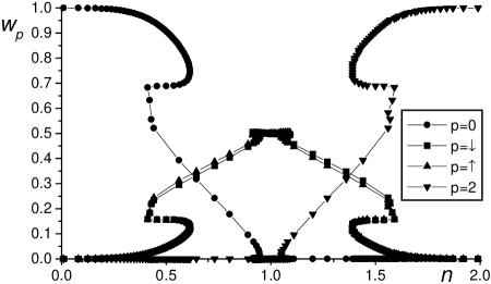
Figure 3: Statistical weights of subspaces $w_{p}$ and ferromagnetic $m_{F}$ and antiferromagnetic $m_{AF}$ order parameters vs electron concentration for $U=1.56$, $T=0.14$

At low temperatures, besides the plateau on the concentration dependence of $w_{p}$ for $p=\sigma,\bar{\sigma}$ at half filling, also the plateau for the statistical weights of subspaces $p=0,2$ are developed at low electron and hole concentrations, see Fig. 3. The $p=0$ and $p=2$ components for the low electron or hole concentrations are in the ferromagnetic state, while the non-Fermi-liquid one is antiferromagnetic (AF) close to half-filling [110]. For the intermediate concentration values the picture is very complicated, even frustrated. It is due to the fact that equations for the mean values (200) have several solutions in this region, which, on the other hand, are mutually connected with the dynamical mean field $J_{\sigma}(\omega_{\nu})$. It is difficult to determine the ground state for this, possibly ‘‘pseudo-gap’’, region, which is located between the ferromagnetic and antiferromagnetic phases.

In Fig. 4 we presented the phase diagram $(T,U)$ – the temperature of the AF ordering vs correlation energy $U$, which is in a qualitative agreement with the results of Refs. [21, 111, 23] and reproduces the results of the Hartree–Fock theory and mean field approximation for $U\ll t$ and $U\gg t$, respectively. Our results for the AF critical temperature for small $U$ are higher then the one of the Quantum Monte Carlo simulations [21] by about a factor at three that describes the reduction of the Hartree–Fock solution by the lowest order quantum fluctuations [107].

10.4 Beyond the Hartree–Fock approximation

Self-energy in the Hartree–Fock approximation [see Eq. (201)] describes some self-consistent shift of the initial energy levels and does not depend on the frequency. All other improvements of the expression for self-energy add the frequency dependent contributions. To see this, let us consider the contribution into the mean values from the first diagram in (187). This diagram originates from the following skeletal diagram

(206)

in the diagrammatic expansion for functional $\Phi_{(p)}$. On the other hand, such a skeletal diagram produces additional contribution into the self-energy

(207)

which is frequency dependent. Also, in order to get a self-consistent set of equations, we introduce renormalized bosonic Green’s functions

$$D_{20(p)}(\omega_{m})=\frac{1}{\mathrm{i}\omega_{m}-\tilde{\lambda}_{20(p)}}\;;$$

$$D_{\sigma\bar{\sigma}(p)}(\omega_{m})=\frac{1}{\mathrm{i}\omega_{m}-\tilde{\lambda}_{\sigma\bar{\sigma}(p)}}\;,$$

$$\tilde{\lambda}_{20(p)} = \lambda_{20}+U\frac{1}{\beta}\sum_{\nu\sigma}\Psi_{\sigma(p)}(\omega_{\nu})\;,$$ (208)

$$\tilde{\lambda}_{\sigma\bar{\sigma}(p)} = \lambda_{\sigma\bar{\sigma}}+U\frac{1}{\beta}\sum_{\nu}\left(\Psi_{\bar{\sigma}(p)}(\omega_{\nu})-\Psi_{\sigma(p)}(\omega_{\nu})\right)\;.$$

Finally, for the Green’s function (179) we get the general representation

$$G_{\sigma(p)}(\omega_{\nu}) = \Bigl{[}\mathrm{i}\omega_{\nu}+\mu_{\sigma}-Un_{\bar{\sigma}(p)}$$ (209)

$$- \widetilde{\Sigma}_{\sigma(p)}(\omega_{\nu})-J_{\sigma}(\omega_{\nu})\Bigr{]}^{-1}\;,$$

where the Hartree–Fock contribution $Un_{\bar{\sigma}(p)}$ is extracted and $\widetilde{\Sigma}_{\sigma(p)}(\omega_{\nu})$ is a frequency dependent part of the self-energy, which within the considered approximation is equal

$$\widetilde{\Sigma}_{\sigma(p)}(\omega_{\nu})=$$

$$\quad\pm\frac{U^{2}}{\beta}\sum_{\nu^{\prime}}\tilde{D}_{\sigma\bar{\sigma}(p)}(\omega_{\nu},\omega_{\nu^{\prime}})\Psi_{\bar{\sigma}(p)}(\omega_{\nu^{\prime}})\;,$$ (210)

where

$$\tilde{D}_{\sigma\bar{\sigma}(p)}(\omega_{\nu},\omega_{\nu^{\prime}})=\left\{\begin{array}[]{cc}D_{20(p)}(\omega_{\nu+\nu^{\prime}})&\mbox{ for }p=0,2\\ D_{\sigma\bar{\sigma}(p)}(\omega_{\nu-\nu^{\prime}})&\mbox{ for }p=\sigma,\bar{\sigma}\end{array}\right.\;.$$ (211)

Now, mean values (185) are equal

$$n_{\sigma(p)} = n^{(0)}_{\sigma(p)}+\frac{1}{\beta}\sum\limits_{\nu}\Psi_{\sigma(p)}(\omega_{\nu})$$ (212)

$$\pm \frac{1}{\beta^{2}}\sum\limits_{\nu\nu^{\prime}}U^{2}\tilde{D}^{2}_{\sigma\bar{\sigma}(p)}(\omega_{\nu},\omega_{\nu^{\prime}})$$

$$\times \Psi_{\sigma(p)}(\omega_{\nu})\Psi_{\bar{\sigma}(p)}(\omega_{\nu^{\prime}})$$

and for the functional (183) in the grand canonical potentials in the subspaces we obtain the following expression

$$\Phi_{(p)} = \frac{1}{\beta^{2}}\sum_{\nu\nu^{\prime}}\left[U\pm U^{2}\tilde{D}_{\sigma\bar{\sigma}(p)}(\omega_{\nu},\omega_{\nu^{\prime}})\right]$$ (213)

$$\times \Psi_{\sigma(p)}(\omega_{\nu})\Psi_{\bar{\sigma}(p)}(\omega_{\nu^{\prime}})\;.$$

Expression (213) besides the Hartree–Fock contribution (202) contains also the contribution from the skeletal diagram (206).

In order to analyze the structure of the poles in (209), an analytical continuation of the expression for $\widetilde{\Sigma}_{\sigma(p)}(\omega_{\nu})$ from the imaginary axis to the real one should be done. To do it, we use the well-known identity

$$\frac{1}{\beta}\sum_{\nu}\frac{\mathrm{e}^{\mathrm{i}\omega_{\nu}0^{+}}}{\mathrm{i}\omega_{\nu}-\lambda}=\pm n_{\pm}(\lambda)\;,$$ (214)

which follows from (149), and analytical properties of the Green’s function

$$G_{\sigma}(z)=\frac{1}{\pi}\int\limits_{-\infty}^{+\infty}\!\!\mathrm{d}\omega\frac{\Im G_{\sigma}(\omega-\mathrm{i}0^{+})}{z-\omega}\;.$$ (215)

Green’s functions in the subspaces $G_{\sigma(p)}(z)$, irreducible parts $\Xi_{\sigma(p)}(z)$, and dynamical mean-field $J_{\sigma}(z)$ all possess the same analytical properties. Finally, we get the following expressions:

$$\tilde{\Sigma}_{\sigma(p)}(z) = \pm\frac{U^{2}}{\pi}\int\limits_{-\infty}^{+\infty}\!\!\mathrm{d}\omega\;n_{+}(\omega)\;\frac{\Im\Psi_{\bar{\sigma}(p)}(\omega-\mathrm{i}0^{+})}{z+\omega-\tilde{\lambda}_{20(p)}}$$ (216)

$$\mp n_{-}(\tilde{\lambda}_{20(p)})\;U^{2}\Psi_{\bar{\sigma}(p)}(\tilde{\lambda}_{20(p)}-z)$$

for subspaces $p=0,2$ and

$$\tilde{\Sigma}_{\sigma(p)}(z) = \pm\frac{U^{2}}{\pi}\int\limits_{-\infty}^{+\infty}\!\!\mathrm{d}\omega\;n_{+}(\omega)\;\frac{\Im\Psi_{\bar{\sigma}(p)}(\omega-\mathrm{i}0^{+})}{z-\omega-\tilde{\lambda}_{\sigma\bar{\sigma}(p)}}$$

$$\mp\left[n_{-}(\tilde{\lambda}_{\sigma\bar{\sigma}(p)})+1\right]\,U^{2}\Psi_{\bar{\sigma}(p)}(z-\tilde{\lambda}_{\sigma\bar{\sigma}(p)})$$

for $p=\sigma,\bar{\sigma}$. Analytical continuation of expressions (212) and (213) can be done in the same way. One can see, that contributions (216) and (10.4) diverge in the paramagnetic phase close to half filling when $\tilde{\lambda}_{20(p)}=0$ and $\tilde{\lambda}_{\sigma\bar{\sigma}(p)}=0$, respectively, which is an unphysical result.

So, we cannot include into the consideration only one contribution from diagram (206) but one have to consider, besides the fermionic loops, also the bosonic ones [112] which correspond to the creation and annihilation of the doublons (pairs of electrons), described by the $\hat{X}^{20}$ and $\hat{X}^{02}$ operators, for subspaces $p=0,2$ and magnons, described by the $\hat{X}^{\uparrow\downarrow}$ and $\hat{X}^{\downarrow\uparrow}$ operators, for $p=\uparrow,\downarrow$. The such loop contributions of bosonic excitations can be summed up and one can obtain

$$\Phi_{(p)} = \frac{1}{\beta}\sum_{m}\ln\bigl{[}1-U$$ (218)

$$\times \left(1\pm U\tilde{D}_{\sigma\bar{\sigma}(p)}(\omega_{m})\right)\tilde{\chi}_{\sigma\bar{\sigma}(p)}(\omega_{m})\bigr{]}\;,$$

where

$$\tilde{D}_{\sigma\bar{\sigma}(p)}(\omega_{m}) = D_{20(p)}(\omega_{m})\;,$$ (219)

$$\tilde{\chi}_{\sigma\bar{\sigma}(p)}(\omega_{m}) = -\frac{1}{\beta}\sum_{\nu}\Psi_{\sigma(p)}(\omega_{\nu})\Psi_{\bar{\sigma}(p)}(\omega_{m-\nu})$$

for subspaces $p=0,2$ and

$$\tilde{D}_{\sigma\bar{\sigma}(p)}(\omega_{m}) = D_{\sigma\bar{\sigma}(p)}(\omega_{m})\;,$$ (220)

$$\tilde{\chi}_{\sigma\bar{\sigma}(p)}(\omega_{m}) = -\frac{1}{\beta}\sum_{\nu}\Psi_{\sigma(p)}(\omega_{\nu})\Psi_{\bar{\sigma}(p)}(\omega_{\nu-m})$$

for subspaces $p=\sigma,\bar{\sigma}$. Expression (213) is the first term of the expansion of functional (218) in the series over $\tilde{\chi}_{\sigma\bar{\sigma}(p)}(\omega_{m})$.

Now we obtain for mean values the following expression

$$n_{\sigma(p)} = n_{\sigma(p)}^{(0)}+\frac{1}{\beta}\sum_{\nu}\Psi_{\sigma(p)}(\omega_{\nu})$$

$$\mp \frac{1}{\beta}\sum_{m}\frac{U^{2}\tilde{D}_{\sigma\bar{\sigma}(p)}^{2}(\omega_{m})\tilde{\chi}_{\sigma\bar{\sigma}(p)}(\omega_{m})}{1-U\left(1\pm U\tilde{D}_{\sigma\bar{\sigma}(p)}(\omega_{m})\right)\tilde{\chi}_{\sigma\bar{\sigma}(p)}(\omega_{m})}$$

and self-energy contains the frequency dependent part

$$\Sigma_{\sigma(p)}(\omega_{\nu})=U\left(n_{\bar{\sigma}(p)}-n_{\bar{\sigma}(p)}^{(0)}\right)+\tilde{\Sigma}_{\sigma(p)}(\omega_{\nu})\;,$$ (222)

$$\tilde{\Sigma}_{\sigma(p)}(\omega_{\nu})=U^{2}\frac{1}{\beta}\sum_{m}$$

$$\frac{\left(1\pm U\tilde{D}_{\sigma\bar{\sigma}(p)}(\omega_{m})\right)\tilde{\chi}_{\sigma\bar{\sigma}(p)}(\omega_{m})\pm\tilde{D}_{\sigma\bar{\sigma}(p)}(\omega_{m})}{1-U\left(1\pm U\tilde{D}_{\sigma\bar{\sigma}(p)}(\omega_{m})\right)\tilde{\chi}_{\sigma\bar{\sigma}(p)}(\omega_{m})}$$

$$\times\left\{\begin{array}[]{rl}\Psi_{\bar{\sigma}(p)}(\omega_{m-\nu}),&\mbox{ for }p=0,2\\ \Psi_{\bar{\sigma}(p)}(\omega_{\nu-m}),&\mbox{ for }p=\sigma,\bar{\sigma}\end{array}\right.\;,$$ (225)

that describes the contributions from the doublons (charge fluctuations) for the Fermi liquid component ($p=0,2$) and magnons (spin fluctuations) for the non-Fermi liquid one ($p=\uparrow,\downarrow$) with the renormalized spectrum determined by the zeros of denominator in (225).

Expression (218) for functional $\Phi_{(p)}$ has the same form as the correction to free energy in the theory of the self-consistent renormalization (SCR) of spin fluctuations by Moriya [113]. But in our case it describes contributions from the single-site bosonic (spin or charge) fluctuations with specific renormalization functions different for different subspaces. Spin fluctuations give the main contribution close to half filling in the non-Fermi liquid regime but for small electron ($n\ll 1$) or hole ($2-n\ll 1$) concentrations the contributions from the charge fluctuations must be taken into account.

11 Concluding remarks

An analytical approaches for the solution of the effective single site problem in the DMFT method for the Hubbard-type models described in this article are based on the strong coupling scheme that considers the strong local interaction as reference system. For the first one, it corresponds to the selection of the Hubbard operators as basis for the projection procedure for Green’s functions while in the second one the perturbation theory over electron hopping is used. Both of them have their advantages.

The equation of motion method together with the averaging over the auxiliary Fermi field gives an approximate interpolating scheme that in specific cases includes a number of known approximations for the Hubbard and similar models. An examples where the proposed approach gives exact results are given (Falicov–Kimball and simplified pseudospin-electron models).

At the same time, the applied procedure of the irreducible Green’s functions introduction and different time decoupling appears to be too simple to obtain the 4-pole structure for the single-site electron Green’s function. An inclusion only of the Fermi-type single-site Hubbard operators in the basis at the formulation of the equations of motion produces the 2-pole Green’s function and only the extension of the basis and application of the projection and decoupling procedures to the higher order functions probably can be able to reveal the more complicated structure of function $G_{\sigma}^{(a)}(\omega)$. Besides, this way requires the consideration of the retarded effective interactions formed by the auxiliary $\xi$-field.

Nevertheless, it should be mentioned, that the simplicity and accessibility of such approach based on the equation of motion method makes it attractive for the approximate analytical considerations. It seems useful to apply it to the problems which have been considered up to now by means of numerical methods (or can be solved exactly only numerically). It should be noted, that the calculation of the electron mean occupation values (and derivation of the equation for the chemical potential), as well as the determination of the grand canonical potential within the equation of motion scheme for the Green’s functions are elucidated only partially in this work. It will be the subject of a separate publication.

The second approach considered in this article uses for the Hubbard-type models a finite-temperature perturbation theory scheme in terms of electron hopping, which is based on the Wick’s theorem for Hubbard operators and is valid for arbitrary values of $U$ ($U<\infty$). Diagrammatic series contain single-site vertices, which are irreducible many-particle Green’s functions for unperturbated single-site Hamiltonian, connected by hopping lines. Applying the Wick’s theorem for Hubbard operators has allowed us to calculate these vertices and it is shown that for each vertex the problem splits into subspaces with ‘‘vacuum states" determined by the diagonal (projection) operators and only excitations around these ‘‘vacuum states" are allowed. The vertices possess a finite $U\to\infty$ limit when diagrammatic series of the strong-coupling approach [76, 77] are reproduced. The rules to construct diagrams by the primitive vertices are proposed.

In the limit of infinite spatial dimensions the total auxiliary single-site problem exactly (naturally) splits into subspaces (four for Hubbard model) and a considered analytical scheme allows to build a self-consistent Baym–Kadanoff-type theory for the Hubbard model. Some analytical results are given for simple approximations: an alloy-analogy approximation, when two-pole structure for Green’s function is obtained, which is exact for the Falicov–Kimball model, and the Hartree–Fock-type approximation, which results in the four-pole structure for the Green’s function. Expanding beyond the Hartree–Fock approximation calls for the considering of the frequency dependent contributions into the self-energy connected with the self-consistently renormalized spin and charge fluctuations.

In general, the expression

$$G^{(a)}_{\sigma}(\omega_{\nu})=\!\sum_{p}\frac{w_{p}}{\mathrm{i}\omega_{\nu}+\mu_{\sigma}-Un_{\bar{\sigma}(p)}-\widetilde{\Sigma}_{\sigma(p)}(\omega_{\nu})-J_{\sigma}(\omega_{\nu})}$$ (226)

gives an exact four-pole structure for the single-site Green’s function of the effective atomic problem. In (174) zero-order Green’s functions (157) are the same for the subspaces $p=0,\sigma$ and $p=2,\bar{\sigma}$, respectively, and correspond to the two-pole solution of the one-site problem without hopping. Switching on of the electron hopping splits these two poles and the value of splitting is determined by the values of the self-energy parts in the subspaces, which describe the contributions from the different scattering processes. Alloy-analogy approximation neglects such scattering processes ($\Sigma_{\sigma(p)}(\omega_{\nu})=0$) which results in the two-pole structure for the Green’s functions (197). But, in general, Green’s functions possess four-pole structure and even the Hartree–Fock approximation (203) clearly shows it.

It should be noted that the four-pole structure of the Green’s function for the atomic problem might not result in the four bands of the spectral weight function (see Fig. 1). The presented consideration allows us to suppose that each pole describes contributions from the different components (subspaces) of the electronic system: Fermi liquid (subspaces $p=0,2$) and non-Fermi liquid ($p=\uparrow,\downarrow$), and for small electron and hole concentrations ($n<2/3$ and $2-n<2/3$) the Fermi-liquid component gives the main contribution (‘‘overdoped regime’’ of high-$T_{c}$’s), whereas in other cases the non-Fermi liquid one (‘‘underdoped regime’’).

12 Acknowledgement

This work was partially supported by the Fundamental Researches Fund of the Ministry of Ukraine for Science and Education (Project No. 02.07/266).

Figure 1: Spectral weight function $\rho_{\sigma}(\omega)$ (205): total and for each subspace, for the different chemical potential values: (a) $\mu=U/2$, $n=1$; (b) $\mu=-1$, $n=0.07$; (c) $\mu=0.01$, $n=0.72$; (d) $\mu=-0.01$, $n=0.66$ ($U=4$, $T=0.2$)

Figure 2: Statistical weights of the subspaces $w_{p}$ (171) as functions of the electron concentration ($U=4$, $T=0.2$)

 

Figure 4: Phase diagram $(T,U)$ at half-filling $n=1$ (AF – antiferromagnetic phase, PM – paramagnetic phase)

References

• [1] E. Dagotto. Rev. Mod. Phys. 66, 763 (1994).
• [2] W. Metzner, D. Vollhardt. Phys. Rev. Lett. 62, 324 (1989).
• [3] E. Müller-Hartmann. Z. Phys. B. 74, 507 (1989).
• [4] W. Metzner. Phys. Rev. B 43, 8549 (1991).
• [5] A. Georges, G. Kotliar. Phys. Rev. B 45. 6479 (1992).
• [6] M. Jarrel. Phys. Rev. Lett. 69, 168 (1992).
• [7] V. Janis̆, D. Vollhardt. Int. J. Mod. Phys. B 6, 731 (1992).
• [8] Yu.A. Izyumov. Uspekhi Fizicheskikh Nauk 165, 403 (1995). [Physics–Uspekhi 38, 385 (1995).
• [9] A. Georges, G. Kotliar, W. Krauth, M.J. Rosenberg. Rev. Mod. Phys. 68, 13 (1996).
• [10] Th. Pruschke, W. Metzner, D. Vollhardt. J. Phys.: Condens. Matter. 13, 9455 (2001).
• [11] U. Brandt, C. Mielsch. Z. Phys. B 75, 365 (1989); 79, 295 (1990); 82, 37 (1991).
• [12] A.M. Shvaika. Physica C 341–348, 177-178 (2000); J. Phys. Studies 5, 349 (2001).
• [13] L.M. Falicov, J.C. Kimball Phys. Rev. Lett. 22, 997 (1969).
• [14] M. Rozenberg, X.Y. Zhang, G. Kotliar. Phys. Rev. Lett. 69, 1236 (1992).
• [15] A. Georges, W. Krauth Phys. Rev. Lett. 69, 1240 (1992).
• [16] M. Caffarel, W. Krauth. Phys. Rev. Lett. 72, 1545 (1994).
• [17] Q. Si, M.J. Rozenberg, G. Kotliar, A.E. Ruckenstein. Phys. Rev. Lett. 72, 2761 (1994).
• [18] R. Bulla. Adv. Solid State Phys. 40, 169 (2000).
• [19] A. Georges, W. Krauth. Phys. Rev. B 48, 7167 (1993).
• [20] T. Pruschke, D.L. Cox, M. Jarrell. Europhys. Lett. 21, 593 (1993).
• [21] T. Pruschke, D.L. Cox, M. Jarrell. Phys. Rev. B 47, 3553 (1993).
• [22] P. Kopietz. Physica B 194–196, 271 (1994); J. Phys.: Condens. Matter. 6, 4885 (1994).
• [23] M.J. Rozenberg, G. Kotliar, X.Y. Zhang. Phys. Rev. B 49, 10181 (1994).
• [24] D. Vollhardt, N. Blumer, K. Held, M. Kollar, J. Schlipf, M. Ulmke. Z. Phys. B 103, 283 (1997).
• [25] T. Herrmann, W. Nolting. J. Magn. Magn. Mater. 170, 253 (1997).
• [26] R.M. Noack, F. Gebhard. Phys. Rev. Lett. 82, 1915 (1999).
• [27] J. Schlipf, M. Jarrell, P.G.J. van Dongen, N. Blumer, S. Kehrein, Th. Pruschke, D. Vollhardt. Phys. Rev. Lett. 82, 4890 (1999).
• [28] R. Bulla. Phys. Rev. Lett. 83, 136 (1999).
• [29] R. Bulla, T.A. Costi, D. Vollhardt. Phys. Rev. B 64, 045103 (2001).
• [30] T. Momoi, K. Kubo. Phys. Rev. B 58, R567 (1998).
• [31] P.J.H. Denteneer, M. Ulmke, R.T. Scalettar, G.T. Zimanyi. Physica A 251, 162 (1998).
• [32] J.-M. Robin, A. Romano, J. Ranninger. Phys. Rev. Lett. 81, 2755 (1998).
• [33] R. Pietig , R. Bulla, S. Blawid. Phys. Rev. Lett. 82, 4046 (1999).
• [34] K. Nagai, T. Momoi, K. Kubo. J. Phys. Soc. Jpn. 69, 1837 (2000).
• [35] A. Schiller. Phys. Rev. B 60, 15660 (1999).
• [36] Y. Ono, R. Bulla, A.C. Hewson. Eur. Phys. J. B. 19, 375 (2001).
• [37] Y. Ohashi, Y. Ono. J. Phys. Soc. Jpn. 70, 2989 (2001).
• [38] K. Held, R. Bulla. Eur. Phys. J. B. 17, 7 (2000).
• [39] V. Zlatić, B. Horvatić. Sol. State Commun. 75, 263 (1990).
• [40] J.K. Freericks. Phys. Rev. B 47, 9263 (1993).
• [41] J.K. Freericks, M. Jarrell. Phys. Rev. Lett. 74, 186 (1993).
• [42] H. Schweitzer, G. Czycholl. Phys. Rev. Lett. 67, 3724 (1991).
• [43] G. Moeller, A. Ruckenstein, S. Schmitt-Rink. Phys. Rev. B 46, 7427 (1992).
• [44] J.K. Freericks, T.P. Devereaux. Condens. Matter Phys. 4, 149 (2001); Phys. Rev. B 64, 125110 (2001).
• [45] J.K. Freericks, T.P. Devereaux, R. Bulla. Phys. Rev. B 64, 233114 (2001).
• [46] G. Palsson, G. Kotliar. Phys. Rev. Lett. 80, 4775 (1998).
• [47] K. Held, I.A. Nekrasov, N. Blumer, V.I. Anisimov, D. Vollhardt. Int. J. Mod. Phys. B 15, 2611 (2001).
• [48] K. Held, G. Keller, V. Eyert, D. Vollhardt, V.I. Anisimov. Phys. Rev. Lett. 86, 5345 (2001).
• [49] R. Bulla, M. Potthoff. Eur. Phys. J. B. 13, 257 (2000).
• [50] M. Potthoff. Phys. Rev. B 64, 165114 (2001).
• [51] M. Potthoff, T. Herrmann, T. Wegner, W. Nolting. Phys. Status Solidi (b) 210, 199 (1998).
• [52] F. Gebhard. The Mott Metal-Insulator Transition: Models and Methods (Berlin: Springer-Verlag, 1997).
• [53] J. Hubbard. Proc. Roy. Soc. A 276, 238 (1963).
• [54] A. Dorneich, M.G. Zacher, C. Gröber, R. Eder. Phys. Rev. B 61, 12816 (2000).
• [55] J. Hubbard. Proc. Roy. Soc. A 281, 401 (1964).
• [56] L.M. Roth. Phys. Rev. 184, 451 (1969).
• [57] W. Nolting, W. Borgiel. Phys. Rev. B 39, 6962 (1989).
• [58] A.B. Harris, R.V. Lange. Phys. Rev. 157, 295 (1967).
• [59] C. Gröber, M.G. Zacher, R. Eder. Preprint arXiv:cond-mat/9902015
• [60] S. Pairault, D. Sénéchal, A.-M.S. Tremblay. Phys. Rev. Lett. 80, 5389 (1998); Preprint arXiv:cond-mat/9905242
• [61] T. Obermeier, T. Pruschke, J. Keller. Phys. Rev. B. 56, 8479 (1997).
• [62] D.M. Edwards, J.A. Hertz. Physica B 163, 527 (1990).
• [63] S. Wermbter, G. Czycholl. J. Phys.: Condens. Matter. 6, 5439 (1994); 7, 7335 (1995).
• [64] H. Kajueter, G. Kotliar. Phys. Rev. Lett. 77, 131 (1996).
• [65] T. Wegner, M. Potthoff, W. Nolting. Phys. Rev. B 57, 6211 (1998).
• [66] T. Herrmann, W. Nolting. Phys. Rev. B 53, 10579 (1996).
• [67] M. Potthoff, T. Herrmann, W. Nolting. Eur. Phys. J. B 4, 485 (1998).
• [68] V. Janis̆. J. Phys.: Condens. Matter 10, 2915 (1998).
• [69] I.V. Stasyuk. // Condens. Matter Phys. 3, 437 (2000).
• [70] A.M. Shvaika. Phys. Rev. B 62, 2358 (2000); 62, 13232 (2000).
• [71] S.P. Cojocaru, V.A. Moskalenko. Teor. Mat. Fiz. 97, 270(1993). [Theor. Math. Phys. USSR 97, 1290 (1993)].
• [72] V.A. Moskalenko, L.Z. Kon. Condens. Matter Phys. 1, 23 (1998).
• [73] Yu.A. Izyumov, N.I. Chashchin. Condens. Matter Phys. 1, 41 (1998).
• [74] P.M. Slobodjan, I.V. Stasyuk. Teor. Mat. Fiz. 19, 423(1974). [Theor. Math. Phys. USSR 19, 616 (1974)].
• [75] Yu.A. Izyumov, Yu.N. Skryabin. Statistical Mechanics of Magnetically Ordered Systems (New York: Consultants Bureau, 1989).
• [76] Yu.A. Izyumov, B.M. Letfulov. J. Phys.: Condens. Matter 2, 8905 (1990).
• [77] Yu.A. Izyumov, B.M. Letfulov, E.V. Shipitsyn, M. Bartkowiak, K.A. Chao. Phys. Rev. B 46, 15697 (1992).
• [78] G. Baym, L.P. Kadanoff. Phys. Rev. 124, 287 (1961).
• [79] G. Baym. Phys. Rev. 127, 1391 (1962).
• [80] P.G.J. van Dongen. Phys. Rev. B 50, 14016 (1994).
• [81] M.H. Hettler, A.N. Tahvildar-Zadeh, M. Jarrel. Phys. Rev. B 58, 7475 (1998).
• [82] B. Velicki, S. Kirpatrick, H. Ehrenreich. Phys. Rev. 175, 741 (1968).
• [83] H. Ehrenreich, L.M. Schwartz. Solid State Physics 31, 150 (1976).
• [84] I.V. Stasyuk, A.M. Shvaika. J. Phys. Studies 3, 177 (1999).
• [85] Yu.A. Tserkovnikov. Teor. Mat. Fiz. 7, 260 (1971).
• [86] N.M. Plakida. Phys. Lett. A 43, 471 (1973).
• [87] N.M. Plakida. Statistical physics and quantum field theory (Ed. by N.N. Bogolubov. M: Nauka, 1973. – P. 205).
• [88] I.V. Stasyuk, O.D. Danyliv. Phys. Status Solidi (b) 219, 299 (2000).
• [89] N.M. Plakida, V.Yu. Yushankhai, I.V. Stasyuk. Physica C 160, 80 (1989).
• [90] B.M. Letfulov. Eur. Phys. J. B 4, 447 (1998).
• [91] B.M. Letfulov. Eur. Phys. J. B 11, 423 (1999).
• [92] Ch. Gruber. Preprint arXiv:cond-mat/9811299.
• [93] J.K. Freericks. Phys. Rev. B 48, 14797 (1993).
• [94] J.K. Freericks, Ch. Gruber, N. Macris. Phys. Rev. B 60, 1617 (1999).
• [95] J.K. Freericks, R. Lemański. Phys. Rev. B 61, 13438 (2000).
• [96] J.K. Freericks, E.H. Lieb, D. Ueltschi. Phys. Rev. Lett. 88, 106401 (2002).
• [97] J. Mustre de Leon, S.D. Conradson, L. Batistic, A.R. Bishop, I.D. Raistrick, M.C. Aronson, F.H. Garzon. Phys. Rev. B 45, 2447 (1992).
• [98] A.P. Saiko, V.E. Gusakov. JETP 108, 757 (1995).
• [99] M. Gutmann, S.J.L. Billinge, E.L. Brosha, G.H. Kwei. Preprint arXiv:cond-mat/9908365.
• [100] K.A. Müller. Z. Phys. B 80, 193 (1990).
• [101] J.E. Hirsch, S. Tang. Phys. Rev. B 40, 2179 (1989).
• [102] M. Frick, W. von der Linden, I. Morgenstern, H. Raedt. Z. Phys. B 81, 327 (1990).
• [103] I.V. Stasyuk, A.M. Shvaika, E. Schachinger. Physica C 213, 57 (1993).
• [104] I.V. Stasyuk, A.M. Shvaika. Ferroelectrics 192, 1 (1997).
• [105] I.V. Stasyuk, A.M. Shvaika, K.V. Tabunshchyk. Condens. Matter Phys. 2, 109 (1999).
• [106] I.V. Stasyuk, A.M. Shvaika, K.V. Tabunshchyk. Ukr. J. Phys. 45, 520 (2000).
• [107] P.G.J. van Dongen, J.A. Vergés, D. Vollhardt. Z. Phys. B 84, 383 (1991).
• [108] C. Gros, W. Wenzel, Valentí, G. Hülsenbeck, J. Stolze. Europhys. Lett. 27, 299 (1994).
• [109] C. Gros, W. Wenzel. Eur. Phys. J. B 8, 569 (1999).
• [110] A.M. Shvaika. Condens. Matter Phys. 4, 85 (2001).
• [111] Y. Kakehashi, H. Hasegawa. Phys. Rev. B 37, 7777 (1988).
• [112] A.M. Shvaika. Acta Physica Polonica B 32, 3415 (2001).
• [113] T. Moriya. Spin Fluctuations in Itinerant Electron Magnetism (Berlin, Heidelberg: Springer-Verlag, 1985; Moscow: Mir, 1988).
Refer to caption Refer to caption