THEORIES OF THE STRUCTURAL GLASS TRANSITION

1 Introduction

Equilibrium phase transitions, e.g. the transition at 0^∘C from water to an ice-crystal, are common phenomena in nature. Such phase transitions between a disordered high temperature phase and an ordered low temperature one are rather well understood and can be theoretically described within statistical mechanics. Given the interaction between the species (particles, spins, etc.) the partition function can be calculated, in principle. Its logarithm yields, e.g. for a canonical ensemble, the free energy which is singular at the equilibrium transition point. This allows to fix this point from first principles.

Besides such order-disorder transitions there also exist transitions between disordered phases. Excluding liquid-liquid transitions these will be called glass transitions. A prominent example is the transition from a supercooled melt of SiO₂-molecules to an amorphous phase which is the well-known “window glass”. One distinguishes two types of glass transitions: spin glass transitions 1rs ; 2rs and structural glass transitions 3rs ; 4rs ; 5rs ; 6rs . Their main difference is that the former occur mostly in systems with quenched disorder and for the latter the disorder is self-generated. We stress that this classification should not be taken too strict since there are also models without quenched disorder showing spin glass behavior 7rs . Typical systems undergoing a structural glass transition are liquids, particularly molecular liquids, like the famous example of SiO₂. In recent years investigations of specific spin glass models, e.g. Potts glass and so-called $p$-spin models with $p\geq 3$ where $p$ spins are coupled by randomly frozen-in (i.e. quenched) infinite range interactions, have revealed some similarities with structural glasses 8rs . We will come back to this point in the 4th chapter.

In contrast to conventional order-disorder transitions, glass transitions are less well understood. There is a broad consensus that a spin glass transition exists and that an appropriately disorder-averaged free energy is singular at the transition point in case of mean field models, i.e. models with infinite range interactions or infinite dimensions. But this is less obvious for short range interactions. The situation for the structural glass transition is even less satisfactory, although substantial progress has been made in the last two decades.

In this article we will mainly focus on the structural glass transition. Spin glass behavior and spin glass transition will be discussed in this monograph by H. Horner. For further details and references on spin glasses, the reader may consult his contribution.

As mentioned above, structural glasses can be obtained by cooling a liquid. In order to bypass crystallization one has to choose a finite cooling rate. For good glassformers, like SiO₂, this rate can be rather modest whereas bad glassformers, like most metallic glasses, require extremely high cooling rates. Under such a cooling process the shear viscosity $\eta(T)$ increases. Close to the so-called calorimetric glass transition temperature $T_{g}$ the supercooled liquid falls out of equilibrium and becomes a glass. At $T_{g}$ thermodynamical quantities like density $n(T)$, specific heat $c_{p}(T)$ at constant pressure, etc. show cross-over behavior, i.e. the slope of $n(T)$ and $c_{p}(T)$ make a more or less well pronounced jump, depending on the cooling rate. $T_{g}$ itself depends on the cooling rate, too. Although $T_{g}$ plays an important practical role, it is less interesting from a fundamental point of view, due to its cooling rate dependence. Besides $T_{g}$ there are at least three more characteristic temperatures $T_{0},T_{K}$ and $T_{c}$. For many glass formers, $\eta(T)$ can be fitted by the Vogel-Fulcher-Tammann law

$$\eta(T)=C\exp\frac{A}{k_{B}(T-T_{0})}\quad,\;T\geq T_{0}$$ (1)

with $A>0$ and $C>0$. The shear viscosity diverges at $T_{0}$. Extrapolating the excess entropy $S_{\textrm{excess}}(T)$ of the supercooled liquid with respect to the crystalline phase to lower temperatures there is the so-called Kauzmann temperature $T_{K}$ at which $S_{\textrm{excess}}$ vanishes:

$$S_{\textrm{excess}}(T_{K})=0\quad.$$ (2)

Since it is argued that a disordered phase should not have a smaller entropy than the crystalline one, $S_{\textrm{excess}}$ can not become negative. Therefore, the system has to undergo a static glass transition at $T_{K}$. This conclusion, however, is not compelling, since there exists inverse melting, i.e. liquids freeze when heated or crystals melt when cooled 9rs . In that case the total entropy of the crystal is higher than that of the liquid. A recent discussion of the Kauzmann problem can be found in Ref. 10rs . $T_{g},T_{0}$ and $T_{K}$ have played an essential role for many decades. In 1984 quite a new theoretical approach, the mode coupling theory 11rs , has shown that there is a critical temperature $T_{c}$, at which a dynamical glass transition takes place. One of the main features is that the nonergodicity parameters $f(\vec{q},T)$ which can be considered as glass order parameters change discontinuously at $T_{c}$:

$$f(\vec{q},T)=\left\{\begin{array}[]{r@{\quad, \quad}l}0&T>T_{c}\\ >0&T\leq T_{c}\quad.\end{array}\right.$$ (3)

Since then numerous experimental investigations and computer simulations were stimulated (see reviews 12rs ; 13rs and Ref. 14rs ; 15rs ). They have shown new characteristic dynamical features close to the dynamical glass transition point $T_{c}$ consistent with mode coupling theory (see also the contribution by U. Buchenau in this monograph).

This short exposition of some of the characteristics of glassy behavior should have given a first impression on how diverse the phenomena in the glass transition region can be. Therefore it is obvious that a successful theoretical description which covers all facets is extremely hard. There are mainly two possible theoretical approaches: phenomenological or microscopic ones. Phenomenological theories start from some of the phenomena of glasses, and are named thereafter. Based on these phenomena a theoretical description is developed capable of describing the observed phenomena. In several cases appealing “physical pictures” are used. However, a couple of assumptions are made which are not proven. The predictive power of such phenomenological approaches is rather limited. This is quite different from a microscopic theory. By microscopic we mean that the physical quantities can be calculated from first principles if the interactions between the species are given. Since the glass transition region is located at rather high temperature quantum effects can be neglected. Therefore, a microscopic theory starts from a classical $N$-body problem. The next chapter will discuss some of the phenomenological theories. The major part of this article is devoted to microscopic theories: The 3rd chapter describes mode coupling theory and the 4th chapter the replica theory for structural glasses.

Finally we want to stress that the present contribution presents a selection and does not aim to be complete. This holds mainly for the phenomenological models. We also do not discuss the potential energy landscape“potential energy landscape” approach 16rs which recently has led to new interesting results 17rs ; 18rs . Almost all of them were obtained from computer simulations. It would be desirable to complement these investigations by analytical theories.

2 PHENOMENOLOGICAL APPROACHES

The presentation in this chapter will be rather short. More details and additional phenomenological approaches can be found in the monographs 3rs ; 5rs ; 6rs and in the review 4rs .

2.1 Adam-Gibbs Theory

In 1965 Adam and Gibbs suggested a theory based on the assumption that dynamically cooperative regions occur when decreasing the temperature towards the glass transition point 19rs . The particles in these regions perform cooperative motion, which leads to a reduction of the configurational degrees of freedom. Here we follow the description of Adam-Gibbs theory as given in Ref. 4rs . The basis of that theory is a number of assumptions:

• For given temperature $T$ there are dynamically cooperative regions labeled by $1,\ldots,i,\ldots,n(T)$ with $N_{1}(T),\ldots,N_{i}(T),\ldots,N_{n(T)}(T)$ particles. The number $n(T)$ of regions decreases with decreasing temperature (see Fig. 1). Due to the conservation of $N$, the total number of particles, it is:

  $$\sum\limits_{i=1}^{n(T)}N_{i}(T)=N\quad.$$ (4)

• These regions take two configurations, only. Accordingly the entropy $s$ per region is:

  $$\ s=k_{B}\ln 2\quad.$$ (5)

  The assumptions that each region takes two configurations, only, is not crucial, but it should be a finite number of order one.

• Fluctuations of $N_{i}(T)$ are small, i.e. it is:

  $$N_{i}(T)\approx N_{0}(T)=N/n(T)\quad.$$ (6)

  because of Eq. (4).

  With these three assumptions we can relate the average number $N_{0}(T)$ of particles within a dynamically cooperative region to the configurational entropy:

  $$S_{c}(T)=k_{B}\ln\,[{\textrm{number of total configurations}}]\quad.$$ (7)

  \begin{picture}(11.0,6.0)\centerline{\hbox{\psfig{angle=-90,width=284.52756pt}}} \end{picture}

  

  Figure 1: Illustration of dynamically cooperative regions (one of them is shown as hatched). Left part: high temperature; right part: low temperatures

  With $2^{n(T)}$, the number of total configurations we get from Eq. (7) by use of Eq. (6):

  $$N_{0}(T)=Nk_{B}\ln 2/S_{c}(T)$$ (8)

  i.e. $N_{0}(T)$ and therefore the size of those regions is inversely proportional to the configurational entropy. This is plausible since the number of possible configurations decreases with increasing $N_{0}(T)$.

  The next important steps are to assume:

• There is a temperature $T_{K}$ at which $N_{0}(T)$ becomes infinite (for $N=\infty$), Then Eq. (8) implies

  $$S_{c}(T)=\left\{\begin{array}[]{ll}>0\quad,\quad T>T_{K}\\ =0\quad,\quad T\leq T_{K}\quad,\\ \end{array}\right.$$ (11)

  i.e  $T_{K}$ is the Kauzmann temperature 20rs .

• The transition between both configurations of a region is an activated process with an activation energy:

$$E(T)=e_{0}N_{0}(T)$$ (12)

where $e_{0}$ may be weakly $T$-dependent. Then the transition time $\tau(T)$ is given by:

$$\tau(T)\sim\exp(\beta E(T))=\exp(\beta e_{0}N_{0}(T))\quad.$$ (13)

Substituting $N_{0}$ from Eq. (8), we arrive at:

$$\tau(T)\sim\exp\left[\frac{e_{0}N\ln 2}{TS_{c}(T)}\right].$$ (14)

Assuming that $S(T)$ vanishes linearly at $T_{K}$ we obtain from Eq. (14) the Vogel-Fulcher-Tammann law close to $T_{K}$:

$$\tau(T)\sim\exp\left[\frac{e_{0}N\ln 2}{T_{K}S^{\prime}_{c}(T_{K})(T-T_{K})}\right]$$ (15)

with $T_{0}=T_{K}$.

This example demonstrates that the appealing picture of dynamically cooperative regions in combination with several assumptions allows to derive the Vogel-Fulcher-Tammann law. But it also shows that no additional predictions are made. Furthermore, it is obvious that the growth of the dynamically cooperative regions would be accomplished by a divergent length scale, which, however, has never been found in experiments or computer simulations.

\begin{picture}(11.0,12.0)\centerline{\hbox{\psfig{angle=0,width=256.0748pt}}} \end{picture}

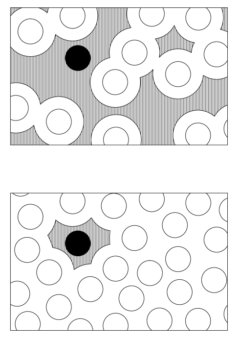
Figure 2: Illustration of the free volume of one sphere (full circle) within a fixed configurations of other spheres (open circles). The free volume is shown as hatched regions. Upper panel: $T>T_{0}$ for which the free volume forms a percolation cluster. Lower panel: $T<T_{0}$ for which the free volume does not percolate but gets localized.

2.2 Free-volume theory

This phenomenological description has been made by Cohen and Turnbull in 1959 21rs . In order to illustrate their idea we choose a system of hard spheres with average density $n$. Let us fix the positions of all spheres except of the $i$-th sphere. Then the $i$-th sphere can move freely in the so-called free volume $\upsilon_{f}(i)$ (see Fig. 2). Although $\upsilon_{f}(j)$ is correlated with $\upsilon_{f}(i)$ for $i\neq j$ one assumes:

• Every sphere has a free volume $\upsilon_{f}$:

  $$i\rightarrow\upsilon_{f}(i)$$ (16)

• $\upsilon_{f}(i)$ are independent random numbers with probability density $p(\upsilon_{f})$ which is assumed to be exponential:

  $$p(\upsilon_{f})=\mathcal{N}\exp(-\upsilon_{f}/\bar{\upsilon}_{f})$$ (17)

  with the mean free volume per particle:

  $$\bar{\upsilon}_{f}=\frac{1}{N}\sum\limits_{i=1}^{N}\upsilon_{f}(i)$$ (18)

  where $\mathcal{N}$ is a normalization constant.

• It is obvious that $\upsilon_{f}(i)$ and therefore $\bar{\upsilon}_{f}$ decreases with increasing density or decreasing temperature (in case of “soft” particles). An essential assumption is that there is a temperature $T_{0}>0$ such that the mean free volume vanishes at $T_{0}$:

  $$\bar{\upsilon}_{f}(T)=\left\{\begin{array}[]{ll}\alpha(T-T_{0})\,\,\,\ ,\,\,\,\ T\geq T_{0}\\ \,\,\,\ 0\,\,\,\ \,\,\,\ \,\,\,\ \,\,\,\ \,\,\,\ ,\,\,\ T<T_{0}\\ \end{array}\right.$$ (21)

  with $\alpha$ the expansion coefficient.

• The inverse shear viscosity is proportional to the probability that the free volume per particle is larger than a certain value $\upsilon_{f}^{*}$ , i.e.:

$$\eta^{-1}(T)\sim\int\limits_{\upsilon_{f}^{*}}^{\infty}\,d\upsilon_{f}p(\upsilon_{f}).$$ (22)

Substituting Eq. (17) and Eq. (21) into Eq. (22) we get the Vogel-Fulcher-Tammann law:

$$\eta(T)\sim\exp\left[\frac{\upsilon^{*}_{f}}{\alpha(T-T_{0})}\right].$$ (23)

2.3 Extended free-volume theory

The free volume theory has been extended by Cohen and Grest 22rs . The main idea of this extension is to make a connection between the glass transition and percolation. If the density $n$ (temperature $T$) is below $n_{g}$ (above $T_{g}$) the individual free volumes $\upsilon_{f}(i)$ overlap or, in other words, the free volume percolates in such a way that a (macroscopic) percolation cluster exists (see upper panel of Fig. 2). In this case a particle can move macroscopic distances, i.e the diffusion constant is finite. Now, increasing $n$ (decreasing $T$) there may exist a critical value $n_{g}$ (or $T_{g})$ at which the percolation cluster disappears which implies that the particles become localized in a glass phase with zero diffusion (see lower panel of Fig. 2). If this scenario would be correct the glass transition point would coincide with the percolation threshold of the free volumes $\upsilon_{f}(i)$. Since percolation is well understood 23rs this relationship would imply several characteristic features, e.g. the fractal nature of the percolation cluster, close to $n_{g}$ (or $T_{g}$). However, there is no experimental evidence for such a fractal behavior. The main critique on the free volume theory is that the density used in the lower panel of Fig. 2 to demonstrate the localization of the free volume still corresponds to a liquid. Computer simulations show that the density of a liquid of e.g. hard discs is already higher than that used in the lower panel of Fig. 2. Accordingly, the free volume, as defined above, is already localized in the liquid phase.

2.4 Gibbs-DiMarzio theory

This approach is not really phenomenological. But the model which has been studied by Gibbs and DiMarzio is very special and has a limited range of applicability. Therefore it is included in this chapter. The model by Gibbs and DiMarzio is capable to explain the vanishing of the configurational entropy 24rs . A system with $N$ polymers on a cubic lattice with $N_{s}$ lattice sites is considered. Each polymer consists of $l$ monomers and can form conformations labeled by $1,2,\cdots,i,\cdots.$ Let $n_{i}$ be the number of polymers with conformation $i$ and $P(\{n_{i}\},N,N_{s})$ the probability that $N$ polymers on a lattice with $N_{s}$ sites built a set $\{n_{i}\}$ of conformations. Associating an energy $\varepsilon_{i}$ with each individual conformation the total energy $E$ is given by:

$$E=\sum\limits_{i}n_{i}\varepsilon_{i}\quad.$$ (24)

Then the number of configurations $\Omega(E,N,N_{s})$ with energy $E$ is:

$$\Omega(E,N,N_{s})=\sum\limits_{\{n_{i}\}}\,P(\{n_{i}\},N,N_{s})\,\,\delta(E-\sum\limits_{i}\varepsilon_{i}n_{i})$$ (25)

from which one obtains the configurational entropy:

$$S_{c}(E,N,N_{s})=k_{B}\,\ln\Omega(E,N,N_{s})\quad.$$ (26)

Of course, the nontrivial problem is to determine $P$ and to perform the sum over $\{n_{i}\}$ in Eq. (25). Making use of a mean field approximation due to Flory and Huggins 25rs one finally gets a critical energy $E_{K}$, which corresponds to the Kauzmann temperature $T_{K}$ with:

$$S_{c}(E,N,N_{s})=\left\{\begin{array}[]{ll}>0\quad,\quad E>E_{K}\\ =0\quad,\quad E\leq E_{K}\quad.\end{array}\right.$$ (29)

Since mean field approximations tend to produce phase transitions even for systems which do not show such transitions, the validity of results Eq. (29) is not obvious.

3 MICROSCOPIC THEORY: MODE COUPLING THEORY

We hope that the short presentation in the 2nd chapter has demonstrated that the status of those phenomenological theories is not satisfactory. Although, plausible “physical pictures” are involved they are based on a couple of crucial assumptions. However, the validity of those remain completely unclear. This demands for a microscopic approach based on first principles. For the first time, such an approach to structural glass transitions was made in 1984 by Bengtzelius, Götze and Sjölander 11rs . Starting from the liquid side these authors applied the mode coupling theory (MCT), developed by Kawasaki 26rs in order to describe the critical slowing down close to a critical point, to the relaxation of the density fluctuations in a supercooled liquid. The result is an equation of motion (see below) for the intermediate scattering function $S(\vec{q},t)$ for a simple liquid which can be measured by neutron- and light scattering (see the contributions by U. Buchenau and J. B. Suck in this monograph). The properties of the solution $S(\vec{q},t)$ of the MCT-equations were mainly investigated in great detail by Götze and his coworkers. These results can be found in the reviews 27rs ; 28rs ; 29rs ; 12rs ; 13rs and in their references. Since most glass formers are molecular systems which involve translational and rotational degrees of freedom, MCT had been extended to a single linear molecule in a simple liquid by Franosch et al. 30rs and to a liquid of linear molecules and arbitrary molecules by Scheidsteger and the author 31rs and by Fabbian et al. 15rs , respectively. This was accomplished by the use of the tensorial formalism which allows the separation of translational and rotational degrees of freedom. Alternatively, one can also use a site-site representation for molecular systems. MCT based on such a description was worked out by Chong and Hirata 32rs and Chong, Götze and Singh 33rs .

Before discussing MCT let us anticipate that the derivation of the MCT-equations requires some more or less strong approximations. Although, these approximations can not be controlled, e.g. due to the lack of a smallness parameter, it is interesting to notice that the MCT-equations for a simple liquid were also obtained by quite different approaches which are the use of generalized fluctuating hydrodynamics by Kirkpatrick 34rs and Das and Mazenko 35rs , density functional theory by Kirkpartick and Wolynes 36rs and recently by the use of the equation of motion for the microscopic density $\rho(\vec{q},t)$ in conjunction with assuming the density fluctuations to be Gaussian by Zaccarelli et al. 37rs . That these quite different approaches lead to the same mathematical structure of the MCT-equations shows its “robustness”. In addition, it has been argued that the MCT-equations become even exact in infinite dimensions 36rs . Further support for MCT comes from a spherical model (without quenched disorder) 38rs and for spin glass models with infinite range interactions (see Ref. 8rs ; 39rs and their references) for which the corresponding $q$-independent MCT-equation has been proven to be exact.

Now we will turn to the discussion of MCT. This will be done in two sections. In the first one we present the derivation of the MCT-equations and in the second one the properties of their solutions.

3.1 Derivation of the MCT-equations

We will restrict ourself to a simple liquid of $N$ identical particles with mass $m$ in a finite volume $V$. We assume two-body interactions $\upsilon(\vec{x}-\vec{x}^{\prime})$ such that the classical hamiltonian is given by:

$$H(\{\vec{x}_{i}\},\{\vec{p}_{i}\})=\sum\limits_{n}\frac{1}{2m}\vec{p}_{n}^{2}+V(\{\vec{x}_{i}\})$$ (30)

with the potential energy:

$$V(\{\vec{x}_{i}\})=\frac{1}{2}\sum\limits_{i\neq j}\upsilon(\vec{x}_{i}-\vec{x}_{j})$$ (31)

$\{\vec{x}_{i}\}$ and $\{\vec{p}_{i}\}$ are the corresponding positions and momenta, respectively. Fixing an initial point $\{\vec{x}_{i}\}$, $\{\vec{p}_{i}\}$ in phase space, the phase space point $\{\vec{x}_{i}(t)\},$ $\{\vec{p}_{i}(t)\}$ at time $t$ is determined by Newtonian’s equation of motion or equivalently by the hermitean Liouville operator:

$$\vec{x}_{i}(t)=e^{i{\cal{L}}t}\vec{x}_{i}\quad,\quad\vec{p}_{i}(t)=e^{i{\cal{L}}t}\vec{p}_{i}\quad.$$ (32)

Of course, one can not solve these equations of motion for a macroscopic system. Therefore one has to use a theoretical framework which restricts itself on the relevant variables. For a liquid this is the microscopic density:

$$\rho(\vec{x},t)=\sum\limits_{n}\delta(\vec{x}-\vec{x}_{n}(t))$$ (33)

where the dependence of the positions $\vec{x}_{n}(t)$ on the initial point $\{\vec{x}_{i}\}$, $\{\vec{p}_{i}\}$ is suppressed. Now we recall that $\rho(\vec{x},t)$ will have a slowly varying part in the strongly supercooled regime, besides fast motions (vibrations) around the quasi-equilibrium positions. Therefore, we can consider $\rho(\vec{x},t)$ or its Fourier transform

$$\rho(\vec{q},t)=\sum_{n}\,e^{i\vec{q}\vec{x}_{n}(t)}=e^{i{\cal L}t}\,\rho(\vec{q})$$ (34)

as a slow variable. If $\rho(\vec{q},t)$ is slow, then the current density

$$\vec{j}(\vec{q},t)=\sum\limits_{n}\,\frac{1}{m}\vec{p}_{n}(t)e^{i\vec{q}\vec{x}_{n}(t)}$$

is slow, too, since it is related to $\rho(\vec{q},t)$ through the continuity equation:

$$\dot{\rho}(\vec{q},t)\equiv i{\cal L}\rho(\vec{q},t)=i\vec{q}\cdot\vec{j}(\vec{q},t)\quad.$$ (35)

We can continue taking time derivatives. Then $\ddot{\rho}(\vec{q},t)$ is given by:

$$\ddot{\rho}(\vec{q},t)=i\vec{q}\cdot\sum\limits_{n}\frac{1}{m}\,\dot{\vec{p}}_{n}(t)\,e^{i\vec{q}\vec{x}_{n}(t)}\,+\,\textrm{kinetic part}\quad.$$ (36)

Using ${\dot{\vec{p}}}_{n}/m=-\partial V(\{\vec{x}_{i}\})/\partial\vec{x}_{n}$ and that Eq. (31) can be

rewritten as

$$V(\{\vec{x}_{i}\})=\frac{1}{2}\,\int d^{3}x\,\int d^{3}x^{\prime}\,\,\upsilon(\vec{x}-\vec{x}^{\prime})\,\rho(\vec{x})\rho(\vec{x}^{\prime})$$

$$=\frac{1}{2V}\,\sum\limits_{\vec{q}}\,\tilde{\upsilon}(\vec{q})\rho^{*}(\vec{q})\,\rho(\vec{q})$$ (37)

it is easy to prove that:

$$\ddot{\rho}(\vec{q},t)=\frac{1}{2V}\sum\limits_{\vec{q}_{1},\vec{q}_{2}}{\!\!\!}^{\prime}w_{0}(\vec{q},\vec{q}_{1},\vec{q}_{2})\,\rho(\vec{q}_{1},t)\,\rho(\vec{q}_{2},t)+\textrm{kinetic part}$$ (38)

with the bare and time-independent vertex:

$$w_{0}(\vec{q},\vec{q}_{1},\vec{q}_{2})=\,\,\,\vec{q}\cdot\left[\vec{q}_{1}\tilde{\upsilon}(\vec{q}_{1})+\vec{q}_{2}\tilde{\upsilon}(\vec{q}_{2})\right].$$ (39)

Here we have used that the Fourier transform $\tilde{\upsilon}(\vec{q})$ of the pair potential is real and $\sum^{\prime}$ denotes summation such that $\vec{q}_{1}+\vec{q}_{2}=\vec{q}$. The result Eq. (38) reveals that the “force” $\ddot{\rho}(\vec{q},t)$ contains contributions from a pair of modes, which are coupled by the bare vertex $w_{0}$. It is rather obvious that the use of a $r$-body interaction would yield a contribution $\rho(\vec{q}_{1},t)\rho(\vec{q}_{2},t)\cdot\ldots\cdot\rho(\vec{q}_{r},t)$. Consequently, the “force” $\ddot{\rho}(\vec{q},t)$ must be slow, as well. By continuing this procedure one obtains a set of slow variables. In the following, however, we will restrict ourself onto the two variables $\rho(\vec{q},t)$ and $j(\vec{q},t)=\vec{q}\cdot\vec{j}(\vec{q},t)/q(q=|\vec{q}|)$, the longitudinal current density. But we have to keep in mind that $\ddot{\rho}(\vec{q},t)$ also is slow. Having chosen $\rho(\vec{q})$ and $j(\vec{q})$ (at $t=0$) as slow variables one can apply the Mori-Zwanzig projection formalism 40rs ; 41rs to derive an exact equation of motion for the normalized intermediate scattering function $\Phi(\vec{q},t)=S(\vec{q},t)/S(\vec{q})$ with

$$S(\vec{q},t)=\frac{1}{N}\langle\rho(\vec{q},t)^{*}\rho(\vec{q})\rangle=\frac{1}{N}\langle\rho^{*}(\vec{q})e^{-i{\cal L}t}\,\rho(\vec{q})\rangle$$ (40)

where we used the hermiticity of ${\cal L}$. $S(\vec{q})$ is the static structure factor which depends on the thermodynamical variables $T,n$, etc. The exact Mori-Zwanzig equation for $\Phi(\vec{q},t)$ reads:

$$\ddot{\Phi}(\vec{q},t)+\Omega_{q}^{2}\,\Phi(\vec{q},t)+\int\limits_{0}^{t}dt^{\prime}\,M(\vec{q},t-t^{\prime})\dot{\Phi}(\vec{q},t^{\prime})=0$$ (41)

with the memory kernel:

$$M(\vec{q},t)=\frac{1}{N}\,\frac{m}{k_{B}T}\,\frac{1}{q^{2}}\langle\ddot{\rho}(\vec{q})^{*}\,Q\,e^{-iQ{\cal L}Qt}\,Q\ddot{\rho}(\vec{q})\rangle$$ (42)

and the microscopic frequencies:

$$\Omega_{q}=\left(\frac{k_{B}T}{m}\,\,\frac{q^{2}}{S(\vec{q})}\right)^{1/2}.$$ (43)

The initial condition is $\Phi(\vec{q},0)=1$, and $\dot{\Phi}(\vec{q},0)=0$ for all $\vec{q}$. The result Eq. (41) makes obvious that the problem to calculate $\Phi(\vec{q},t)$ has been shifted to the calculation of $M(\vec{q},t)$, which seems to be hopeless, as well. But this is not really true. In contrast to $\Phi$ it is possible to approximate the memory kermel $M$. $M(\vec{q},t)$ is the correlation function of the “forces” $Q\,\ddot{\rho}(\vec{q})$, however, with the reduced Liouvillian ${\cal L}^{\prime}=\,Q\,{\cal L}\,Q$. $Q$ is the projector (see below) which projects perpendicular to both slow variables $\rho(\vec{q})$ and $j(\vec{q})$. Since $\ddot{\rho}(\vec{q})$ contains a coupled pair of modes $\rho(\vec{q}_{1})\,\rho(\vec{q}_{2})$ (cf. Eq. (38)) and because $Q\rho(\vec{q}_{1})\,\rho(\vec{q}_{2})\neq 0$, the “force” $Q\ddot{\rho}(\vec{q})$ still contains a slow part. This suggests to use the following approximation 27rs :

$$Q\ddot{\rho}(\vec{q})\rightarrow Q|\ddot{\rho}(\vec{q})\rangle\approx{\cal P}Q|\ddot{\rho}(\vec{q})\rangle$$ (44)

where ${\cal P}$ is the projector onto pairs of modes:

$${\cal P}=\sum\limits_{\vec{q}_{1}\vec{q}_{2},\vec{q}_{1}^{\prime}\vec{q}_{2}^{\prime}}g(\vec{q}_{1}\vec{q}_{2};\vec{q}_{1}^{\prime}\vec{q}_{2}^{\prime})|\rho(\vec{q}_{1})\rho(\vec{q}_{2})\rangle\langle\rho(\vec{q}_{1}^{\prime})^{*}\rho(\vec{q}^{\prime}_{2})^{*}|$$ (45)

and $g$ is determined such that ${\cal P}^{2}={\cal P}$. The reader should note that we have introduced a bra- and ket-notation $\langle|$ and $|\rangle$, respectively, like in quantum mechanics. This can be done since the canonical average $\langle A^{*}B\rangle$ of two phase space functions $A^{*}$ and $B$ can be interpreted as scalar product $\langle A^{*}|B\rangle$. It is the existence of this scalar product which allows to introduce projectors. Substituting Eq. (44) and Eq. (45) into Eq. (42) relates $M(\vec{q},t)$ to the correlation function

$$\langle\rho(\vec{q}_{3}^{\prime})^{*}\rho(\vec{q}_{4}^{\prime})^{*}|e^{-i{\cal L}^{\prime}t}|\rho(\vec{q}_{1})\rho(\vec{q}_{2})\rangle\quad.$$ (46)

This relationship involves $g(\vec{q}_{1}\vec{q}_{2};\vec{q}_{1}^{\prime}\vec{q}_{2}^{\prime})g(\vec{q}_{3}\vec{q}_{4};\vec{q}_{3}^{\prime}\vec{q}_{4}^{\prime})$ and $\langle\ddot{\rho}(\vec{q})^{*}Q|\rho(\vec{q}_{3})\rho(\vec{q}_{4})\rangle\\ \langle\rho(\vec{q}_{1}^{\prime})^{*}\rho(\vec{q}_{2}^{\prime})^{*}|Q\ddot{\rho}(\vec{q}_{1})\rangle$ which are static quantities. Now, the crucial approximation is the factorization of the correlator Eq. (46) and simultaneously replacing ${\cal L}^{\prime}$ by ${\cal L}$:

$$\langle\rho(\vec{q}^{\prime}_{3})^{*}\rho(\vec{q}^{\prime}_{4})^{*}|e^{-i{\cal L}^{\prime}t}|\rho(\vec{q}_{1})\rho(\vec{q}_{2})\rangle\approx$$

$$\approx[\langle\rho(\vec{q}_{1})^{*}|e^{-i{\cal L}t}|\rho(\vec{q}_{1})\rangle\,\langle\rho(\vec{q}_{2})^{*}|e^{-i{\cal L}t}|\rho(\vec{q}_{2})\rangle\delta_{q^{\prime}_{3}q_{1}}\,\delta_{q^{\prime}_{4}q_{2}}+$$

$$+(1\longleftrightarrow 2)]$$

$$=N^{2}S(\vec{q}_{1})S(\vec{q}_{2})\,\,\Phi(\vec{q}_{1},t)\,\Phi(\vec{q}_{2},t)[\delta_{q^{\prime}_{3}q_{1}}\,\delta_{q^{\prime}_{4}q_{2}}+\delta_{q^{\prime}_{3}q_{2}}\,\delta_{q^{\prime}_{4}q_{1}}]\quad.$$ (47)

The condition ${\cal P}^{2}={\cal P}$ implies that $g(\vec{q}_{1}\vec{q}_{2};\vec{q}^{\prime}_{1}\vec{q}^{\prime}_{2})$ is the inverse of the “matrix” $(\langle\rho(\vec{q}^{\prime}_{1})^{*}\rho(\vec{q}^{\prime}_{2})^{*}\rho(\vec{q}_{1})\rho(\vec{q}_{2})\rangle)$. Since this “matrix” equals the correlator Eq. (46) at $t=0$ it is approximated by the r.h.s. of Eq. (3.1), at $t=0$. Using this approximation one immediately finds:

$$g(\vec{q}_{1},\vec{q}_{2};\,\vec{q}^{\prime}_{1},\vec{q}^{\prime}_{2})\approx(4N^{2}S(\vec{q}_{1})S(\vec{q}_{2}))^{-1}[\delta_{q^{\prime}_{1}q_{1}}\,\delta_{q^{\prime}_{2}q_{2}}+\delta_{q^{\prime}_{1}q_{2}}\,\delta_{q^{\prime}_{2}q_{1}}]\quad.$$ (48)

Using $Q=1-{\cal P}=1-(N\,S(\vec{q}))^{-1}|\rho(\vec{q})\rangle\langle\rho(\vec{q})^{*}|-(Nk_{B}T/m)^{-1}|j(\vec{q})\rangle\langle j(\vec{q})^{*}|$ the static correlation $\langle\ddot{\rho}(\vec{q})^{*}\,Q|\rho(\vec{q}_{1})\rho(\vec{q}_{2})\rangle$ can be expressed as follows 27rs :

$$\langle\ddot{\rho}(\vec{q})^{*}Q|\rho(\vec{q}_{1})\rho(\vec{q}_{2})\rangle=N\frac{k_{B}T}{m}\,S(\vec{q}_{1})\,S(\vec{q}_{2})\{-n\vec{q}\cdot[\vec{q}_{1}c(\vec{q}_{1})+\vec{q}_{2}c(\vec{q}_{2})]+$$

$$\qquad\qquad{}+q^{2}[1-\langle\rho(\vec{q})^{*}\rho(\vec{q}_{1})\rho(\vec{q}_{2})\rangle/(N\,S(\vec{q})\,S(\vec{q}_{1})\,S(\vec{q}_{2}))]\}\,\delta_{q_{1}+q_{2},q}$$ (49)

where we introduced the direct correlation function $c(\vec{q})$ defined by $S(\vec{q})=[1-nc(\vec{q})]^{-1}$. Substituting Eqs. (44)-(3.1) into Eq. (42) yields finally the MCT-approximation for the memory kernel:

$$M(\vec{q},t)\approx\nu_{q}\,\delta(t)+\Omega_{q}^{2}m(\vec{q},t)$$ (50)

$$m(\vec{q},t)=\frac{1}{2V}\,\sum\limits_{\vec{q}_{1},\vec{q}_{2}}{\!\!\!}^{\prime}\,V(\vec{q},\vec{q}_{1},\vec{q}_{2})\,\Phi(\vec{q}_{1},t)\,\Phi(\vec{q}_{2},t)$$ (51)

with the positive vertices:

$$V(\vec{q},\vec{q}_{1},\vec{q}_{2})=\frac{1}{n}\,S(\vec{q})\,S(\vec{q}_{1})\,S(\vec{q}_{2})\,q^{-4}\{n\vec{q}\cdot[\vec{q}_{1}c(\vec{q_{1}})+\vec{q}_{2}c(\vec{q}_{2})]-$$

$$-q^{2}[1-\langle\rho(\vec{q})^{*}\rho(\vec{q}_{1})\rho(\vec{q}_{2})\rangle/(N\,S(\vec{q})\,S(\vec{q}_{1})\,S(\vec{q}_{2}))]\}^{2}.$$ (52)

The first term on the r.h.s of Eq. (50) accounts for the fast part of the “force” $Q\ddot{\rho}(\vec{q})$ leading to a frictional contribution.

The equations Eqs. (41), (43) and  (50)- (3.1) are the mode coupling equations. Due to the MCT-approximation they are a closed set of integro-differential equations for the normalized correlator $\Phi(\vec{q},t)$ with initial conditions $\Phi(\vec{q},0)\equiv 1$ and $\dot{\Phi}(\vec{q},0)\equiv 0$, because of time reversal symmetry. As an input they only need the static two-point correlator $S(\vec{q})$ (or equivalently the direct correlation function $c(\vec{q}$)), the static three point correlator $\langle\rho(\vec{q})^{*}\rho(\vec{q}_{1})\,\rho(\vec{q}_{2})\rangle$ and the frictional constants $\nu_{q}$. $\nu_{q}$ which can only be determined from kinetic theory does not influence the glassy behavior. Therefore it can be put to zero. The remaining static two- and three point correlators $S(\vec{q})=\langle\rho(\vec{q})^{*}\rho(\vec{q})\rangle/N$ and $\langle\rho(\vec{q})^{*}\,\rho(\vec{q}_{1})\,\rho(\vec{q}_{2})\rangle$ can be calculated for given potential energy $V(\{\vec{x}_{i}\})$. This is what makes MCT a microscopic first principle theory. Here a comment is in order: MCT will be applied to the supercooled liquid, i.e. to a temperature regime where the stable thermodynamical phase is a crystal. In order to study the glass transition one has to use the static correlators for the supercooled liquid and not for the crystal. MCT allows to predict the time dependence of the density fluctuations provided both static correlators are known. They can be obtained either from analytical approximation schemes 40rs or from experiments and simulations. Application of the convolution approximation 40rs :

$$\langle\rho(\vec{q})^{*}\rho(\vec{q}_{1})\rho(\vec{q}_{2})\rangle\approx N\,\,S(\vec{q})S(\vec{q}_{1})S(\vec{q}_{2})\,\,\delta_{q_{1}+q_{2},q}$$ (53)

leads to a further simplification of the vertices Eq. (3.1):

$$V(\vec{q},\vec{q}_{1},\vec{q}_{2})=nS(\vec{q})S(\vec{q_{1}})S(\vec{q}_{2})\,[\vec{q}\cdot(\vec{q}_{1}c(\vec{q}_{1})+\vec{q}_{2}c(\vec{q_{2}}))]^{2}/q^{4}$$ (54)

which involve $S(\vec{q})$ (or $c(\vec{q})$), only. For SiO₂-liquids it has been demonstrated by Sciortino and Kob 42rs that a satisfactory agreement of, e.g. the critical nonergodicity parameters determined from a MD-simulation with those from MCT is only obtained with the vertices from Eq. (3.1) where the three-point correlator is not factorized. This is rather plausible, because SiO₂ is a covalent glass former with bond orientational correlations which are completely neglected by the convolution approximation Eq. (53).

3.2 Solutions and predictions of MCT

The main question which arises is: How can one detect a glass transition within MCT? The answer is rather simple. Let us use the nonergodicity parameters defined by:

$$f(\vec{q})=\lim\limits_{t\rightarrow\infty}\Phi(\vec{q},t)=-\lim\limits_{z\rightarrow\infty}z\hat{\Phi}(\vec{q},z)\quad.$$ (55)

These parameters, which are just the infinite time limit of $\Phi(\vec{q},t)$ or the zero frequency limit of its Laplace transform

$$\hat{\Phi}(\vec{q},z)=i\int\limits_{0}^{\infty}dt\Phi(\vec{q},t)e^{izt}\quad,\;\textrm{Im}\,z>0$$ (56)

can be used as glass order parameters, because they vanish in an ergodic phase (= liquid phase) and are nonzero in a nonergodic one, which is interpreted as a glass phase. To be more precise, this is true for the correlation function of the density fluctuations $\delta\rho(\vec{q},t)=\rho(\vec{q},t)-\langle\rho(\vec{q},t)\rangle$, only. Since $\delta\rho(0,t)=0$ and $\delta\rho(\vec{q},t)=\rho(\vec{q},t)$ for all $\vec{q}\neq 0$, it is sufficient to investigate $\Phi(\vec{q},t)$. Thus it is:

$$f(\vec{q})=\left\{\begin{array}[]{r@{\quad, \quad}l}0&\textrm{liquid}\\ >0&\textrm{glass}\end{array}\right.$$ (57)

Since $\ddot{\Phi}(\vec{q},t)\rightarrow 0$ for $t\rightarrow\infty$, it is easy to show that Eq. (41) yields a nonlinear set of algebraic equations for $f(\vec{q})$:

$$\frac{f(\vec{q})}{1-f(\vec{q})}={\cal F}[f(\vec{q})]$$ (58)

with:

$${\cal F}[f(\vec{q})]=\frac{1}{2V}\sum\limits_{\vec{q}_{1},\vec{q}_{2}}{\!}^{\prime}\,V(\vec{q},\vec{q}_{1},\vec{q}_{2})f(\vec{q}_{1})f(\vec{q}_{2})\quad.$$ (59)

One can prove that the long time limit $f(\vec{q})$ is distinguished from other possible solutions of Eq. (58), (59) by the following properties 27rs

• $f(\vec{q})$ is real (since $\Phi(\vec{q},t)$ is real)

• $0\leq f(\vec{q})\leq 1$

• If several solutions $f_{1}(\vec{q})>f_{2}(\vec{q})\geq f_{3}(\vec{q})\geq\cdots$ exist, the long time limit is the largest one: $f(\vec{q})=f_{1}(\vec{q})$ .

The positiveness of the vertices is crucial for (iii).

It is obvious from Eqs. (58), (59) that $f(\vec{q})\equiv 0$ is always a solution. In order to check whether a nontrivial solution exists, let us neglect the $q$-dependence for a moment. This leads to a so-called schematic model 27rs , the ${\cal F}_{2}$-model, where ${\cal F}[f]=\upsilon f^{2},\upsilon\geq 0$, i.e. we have to solve

$$\frac{1}{1-f}=vf^{2}\quad.$$ (60)

For $f\neq 0$ this leads to a quadratic equation with solution:

$$f_{1/2}=\frac{1}{2}[1\pm\sqrt{1-4/v}]\quad.$$ (61)

\begin{picture}(11.0,6.0)\centerline{\hbox{\psfig{angle=0,width=341.43306pt}}} \end{picture}

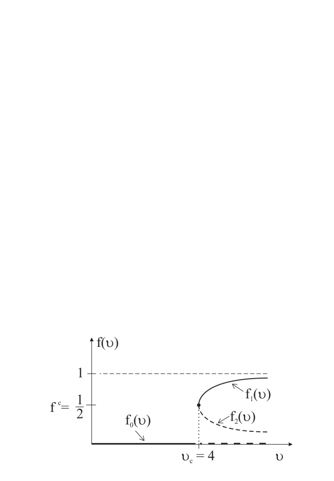
Figure 3: Qualitative control parameter dependence of the nonergodicity parameter of the ${\mathcal{F}}_{2}$-model. $f_{0}(v)\equiv 0$ is the trivial solution. At $v_{c}=4$ two new solutions $f_{1}(v)$ and $f_{2}(v)$ bifurcate.

Since $f_{1/2}$ is not real for $v<v_{c}=4$, the only physical solution in this range is $f_{0}=0$. For $v\geq v_{c}$ two real solutions $f_{1}>f_{2}$ bifurcate from the trivial one. This scenario is illustrated in Fig. 3. Hence, we get for the $F_{2}$-model

$$f(v)=\left\{\begin{array}[]{r@{\quad, \quad}l}0&v<v_{c}\\ \frac{1}{2}[1+\sqrt{1-v_{c}/v}]&v\geq v_{c}\end{array}\ \right.$$ (62)

i.e. at the critical control parameter $v_{c}=4$ the nonergodicity parameter changes discontinuously from zero to the critical nonergodicity parameter $f^{c}=f(\upsilon_{c})=1/2$. This type of transition is called type-B transition, in contrast to a type-A transition which is continuous 27rs . Such a type-A transition occurs, e.g. for the ${\cal F}_{1}$-model: ${\cal F}[f]=\upsilon f$, $\upsilon\geq 0$.

This simple example has shown that an ergodic-to-nonergodic transition can occur at a critical coupling constant $v_{c}$. Since the vertices $V(\vec{q},\vec{q}_{1},\vec{q}_{2})$ are positive and $0\leq f(\vec{q})\leq 1$, ${\cal F}[f(\vec{q})]$ will diverge in the strong coupling limit $V(\vec{q},\vec{q}_{1},\vec{q}_{2})\rightarrow\infty$. Therefore Eq. (58) can only be fulfilled if the nontrivial solution converges to one. Therefore there must be a critical hypersurface in the control parameter space at which transitions from $f(\vec{q})\equiv 0$ to $f(\vec{q})\neq 0$ happen. Because the vertices depend through $S(\vec{q})$ on the thermodynamic variables $T,n$ etc. and increase with decreasing $T$ (increasing $n$) there will be a critical temperature $T_{c}$ (critical density $n_{c}$) at which the system undergoes an ergodic-to-nonergodic transition, i.e. a glass transition. From this we can conclude that MCT yields a dynamical glass transition whereas static quantities, e.g. $S(\vec{q})$, are not singular at $T_{c}$ (or $n_{c}$). Having established the existence of a glass transition singularity, one can study the dynamics close to it. For large times (small frequencies) compared to the microscopic time scale $\Omega_{q}^{-1}(\Omega_{q})$ the Laplace transform of Eq. (41) yields with Eq. (50):

$$\frac{z\hat{\Phi}(\vec{q},z)}{1+z\hat{\Phi}(\vec{q},z)}=z\hat{m}(\vec{q},z)\quad.$$ (63)

Here we used $\nu_{q}=0$. The reader should notice that Eq. (63) does not involve anymore the microscopic frequencies $\Omega_{q}$. The schematic representation of a solution of the MCT-equations Eqs. (41), (50)- (3.1), including the microscopic time regime, is shown in Figure 4. This Figure clearly demonstrates the existence of a critical temperature $T_{c}$ at which a jump of $f(\vec{q})$ occurs. The generic behavior close to $T_{c}$ is given by (cf. also Eq. (62)):

$$f(\vec{q})=\left\{\begin{array}[]{ll}0\,\,\,\ ,\,\,\,\ T>T_{c}\\ f^{c}(\vec{q})+\textrm{const}(T_{c}-T)^{1/2}\,\,,\,\,T\leq T_{c}\\ \end{array}\right.$$ (66)

where the constant is $q$-dependent. We can observe from Figure 4 that close to $T_{c}$ there is a time scale on which the correlator $\Phi(\vec{q},t)$ is close to the critical nonergodicity parameter $f^{c}(\vec{q})=f(\vec{q})|_{{}_{T=T_{c}}}$. This suggests the Ansatz:

$$\Phi(\vec{q},t)=f^{c}(\vec{q})+h(\vec{q})G(t)$$ (67)

with $|G(t)|\ll 1$. It is important to realize that the $q$- and $t$-dependence is factorized. This is related to the type of bifurcation scenario for which the non-degenerated largest eigenvalue of the stability matrix of the linearized Eq. (58) becomes one. Therefore at $T_{c}$ only one unstable eigenvector occurs. The critical amplitude $h(\vec{q})$ is the amplitude of that eigenvector. Substituting Eq. (67) into Eq. (63) and expanding up to quadratic order in $G$ one obtains:

$$\sigma+\lambda\{-zLT[G^{2}(t)](z)\}-\{-z\widehat{G}(z)\}^{2}=0$$ (68)

with the separation parameter

$$\sigma(T)\cong\sigma_{0}(T_{c}-T)=\left\{\begin{array}[]{ll}<0\,\,\,\ ,\,\,\,\ \textrm{liquid}\\ >0\,\,\,\ ,\,\,\,\ \textrm{glass}\\ \end{array}\right.$$ (71)

\begin{picture}(11.0,5.5)\centerline{\hbox{\psfig{angle=-90,width=369.88582pt}}} \end{picture}

Figure 4: Qualitative time- and temperature-dependence of the intermediate scattering function $\Phi(\vec{q},t)$ for fixed $\vec{q}$. The values 0.1 and 0.01 for ($T-T_{c})/T_{c}$ should not be taken literally. They should only indicate that $T$ is chosen closer and closer to $T_{c}$.

($\sigma_{0}$ is positive) and the exponent parameter

$$\lambda=\lambda[S(\vec{q})|_{{}_{T=T_{c}}}]$$ (72)

The separation parameter is a measure of the distance from the transition point. The importance of $\lambda$ will become clear below. Explicit expression for $\sigma$ and $\lambda$ are given in Ref. 27rs .

At the transition point, i.e. for $\sigma=0$, the solution of Eq. (68) is the critical law:

$$G(t)\sim t^{-a}\quad.$$ (73)

where the exponent $a$ is a solution of:

$$\lambda=\frac{\Gamma^{2}(1-a)}{\Gamma(1-2a)}$$ (74)

with $\Gamma(x)$ the Gamma function. Since $\lambda$ is uniquely determined by $S(\vec{q})$ at $T_{c}$ it can be calculated microscopically, from which $a$ follows. $a$ is restricted to $0<a\leq 1/2$. For $a=0$ a higher order bifurcation scenario occurs 27rs . To solve Eq. (68) for $T\neq T_{c}$ it is convenient to introduce a correlation scale $\sqrt{|\sigma|}$ by:

$$G(t)=\sqrt{|\sigma|}\,\,g_{\pm}(t/t_{\sigma})\quad,\quad\sigma\gtrless 0$$ (75)

where the time scale $t_{\sigma}$ and the master functions $g_{\pm}$ can be obtained as follows. Introducing Eq. (75) into Eq. (68) and using $\hat{t}=t/t_{\sigma}$ and $\hat{z}=t_{\sigma}z$ leads to:

$$\pm 1/\hat{z}+\lambda LT[g_{\pm}^{2}(\hat{t})](\hat{z})+\hat{z}(\hat{g}_{\pm}(\hat{z}))^{2}=0$$ (76)

which has the solution:

$$g_{\pm}(\hat{t})\sim\hat{t}^{-a}$$ (77)

for $\hat{t}\ll 1$, i.e.  $t\ll t_{\sigma}$, since $\pm 1/\hat{z}$ can be neglected due to $\hat{z}\gg 1$. Substitution of Eq. (77) into Eq. (75) and taking into account that $G(t)$ must reduce for $\sigma\rightarrow 0$ to the critical correlator Eq. (73) allows to fix $t_{\sigma}$:

$$t_{\sigma}(T)\sim|\sigma|^{-\frac{1}{2a}}\sim|T-T_{c}|^{-\frac{1}{2a}}\quad,\quad T\lessgtr T_{c}\quad.$$ (78)

For $\hat{t}\gg 1$ one obtains 27rs :

$$g_{\pm}(\hat{t})\cong\left\{\begin{array}[]{ll}\sqrt{1-\lambda}\,\,\,\ ,\,\,\,\ (+)\\ -B\hat{t}^{b}\,\,\,\,\,\,\,\,\,\,,\,\,\,\ (-)\\ \end{array}\right.$$ (81)

with $B>0$.

Again, the positive exponent $b$ is determined by the exponent parameter $\lambda$:

$$\lambda=\frac{\Gamma^{2}(1+b)}{\Gamma(1+2b)}\quad.$$ (82)

In the liquid phase (minus sign in Eq. (81)) we obtain, besides the critical law Eq. (73) a second power law, the so-called von Schweidler law. Substituting $g_{-}(\hat{t})$ from Eq. (81) into Eq. (75) leads to

$$G(t)\sim(t/\tau(T))^{b}$$ (83)

with the second time scale:

$$\tau(T)\sim|\sigma|^{-{\frac{1}{2b}}}\,t_{\sigma}\sim(T-T_{c})^{-\gamma}\,,\,\,\,\,T\geq T_{c}$$ (84)

and the exponent

$$\gamma=\frac{1}{2a}+\frac{1}{2b}\quad.$$ (85)

\begin{picture}(11.0,5.5)\centerline{\hbox{\psfig{angle=-90,width=369.88582pt}}} \end{picture}

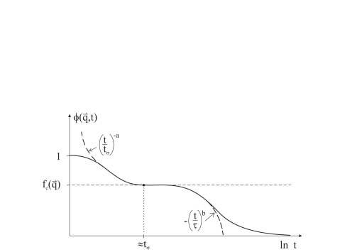
Figure 5: $\Phi(\vec{q},t)$ for fixed $\vec{q}$ and a single temperature $T>T_{c}$ (solid line). Both power laws, the critical law and the von Schweidler law, are shown as dashed lines. The horizontal dashed line is the plateau height equal to the critical nonergodicity parameter $f_{c}(\vec{q})$

The von Schweidler law, Eq. (83), is valid for $\hat{t}\gg 1$, i.e. $t\gg t_{\sigma}(T)$ and $t\ll\tau(T)$ because of $|G(t)|\ll 1$. Both power laws are shown in Figure 5. The critical law describes the relaxation to the plateau value $f^{c}(\vec{q})$ and $f(\vec{q})$ above and below $T_{c}$, respectively, and the von Schweidler law the initial decay from the plateau for $T>T_{c}$. Both time scales $t_{\sigma}$ and $\tau$ exhibit power law divergence at $T_{c}$. $\tau$ diverges faster than $t_{\sigma}$, due to $\gamma>/1(2a)$ (see Fig. 6).

\begin{picture}(11.0,7.0)\centerline{\hbox{\psfig{angle=0,width=341.43306pt}}} \end{picture}

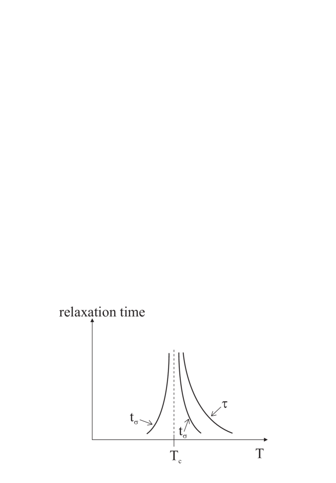
Figure 6: Qualitative T-dependence of both relaxation times $t_{\sigma}(T)$ and $\tau(T)$ which exhibit power law divergence at $T_{c}$

These fascinating results proven by Götze in 1984 43rs and 1985 44rs were absolutely new. The time range $t_{0}\ll t\ll\tau(T)$ ($t_{0}$ is a microscopic time scale $\sim\Omega_{q}^{-1}$) which includes both power laws have been called (fast) $\beta$-relaxation. It has a simple physical explanation. If the temperature is low enough each particle feels a cage on a time scale $t_{\sigma}$. The first relaxation step (critical law) is a relaxation within the cage and the second one (von Schweidler law) is related to the “opening” of the cage for $t\gg t_{\sigma}$ which is the initial stage of the structural relaxation. The fact that the $q$- and $t$-dependence of the correlators factorize in the $\beta$-regime is one of the highly nontrivial predictions of MCT which has not been found before in condensed matter physics. Numerous experiments 12rs (see also the contribution by U. Buchenau in this monograph), and computer simulations 13rs ; 14rs ; 15rs have given consistent results with regard to these MCT-predictions.

What remains is to study the dynamics for $t$ of the order or much larger than $\tau(T)$ which is called $\alpha$-relaxation. There the factorization does not hold anymore. Therefore one has to solve Eq. (63). This can only be done numerically. But there is one important feature, which is the scale invariance of Eq. (63). This means that a scale transformation $t\rightarrow t\cdot y$, $\Phi(\vec{q},t)\rightarrow\Phi(\vec{q},t\cdot y)$ or $z\rightarrow z\cdot y^{-1}$ , $\hat{\Phi}(\vec{q},z)\rightarrow y\hat{\Phi}(\vec{q},z\cdot y^{-1})$ leaves Eq. (63) invariant. This allows to introduce a $q$-dependent master function $\Phi_{q}(\tilde{t})$ such that

$$\Phi(\vec{q},t;T)=\Phi_{q}(t/\tau(T))$$ (86)

i.e. the time and temperature dependence of $\Phi$ appears only in the combination $t/\tau(T)$. Eq. (86) is well-known in the glass science as the time-temperature superposition principle. The master function $\Phi_{q}(\tilde{t})$ can be determined from a numerical solution of Eq. (63). The validity of Eq. (63) and Eq. (86) has also been test experimentally 12rs and by computer simulations 13rs ; 15rs .

4 MICROSCOPIC THEORY: REPLICA THEORY

In 1996 Mézard and Parisi 45rs have presented a replica theory for the structural glass transition. This theory has been inspired by spinglass theory 1rs ; 2rs . Kirkpatrick, Thirumalai and Wolynes first noticed the analogy between spinglass and structural glass transitions 8rs . In 1987 they have shown that mean-field spin glass models with a one-step replica symmetry breaking 2rs exhibit a dynamical (MCT-like)glass transition at $T_{c}$ and a static one at $T_{s}$, which is below $T_{c}$. At $T_{s}$ the configurational entropy vanishes. Hence $T_{s}$ can be identified with $T_{K}$, the Kauzmann temperature. In the next section we will describe the physical picture behind this theory and its thermodynamic formulation. The second section then contains the microscopic theory which can be considered as a first principle approach of an earlier attempt by Singh, Stoessel and Wolynes to describe the glass transition by a density functional theory 46rs .

4.1 Thermodynamical description

Let $\rho(\vec{x})$ be the local particle density of a liquid with $N$ identical particles in a volume $V$. A theorem 47rs guarantees that there exists a free energy functional ${\mathcal{F}}[\rho(\vec{x}),T]$ such that the equilibrium phases are obtained from

$$\frac{\delta{\mathcal{F}[\rho(\vec{x}),T]}}{\delta\rho(\vec{x})}=0$$ (87)

${\mathcal{F}}[\rho(\vec{x}),T]$ is not known exactly. In many cases one uses an approximation suggested by Ramakrishnan and Youssouff 48rs . Let $\rho^{(\alpha)}(\vec{x})$ (T-dependence is suppressed), $\alpha=1,2,3,\ldots$ be solutions of Eq. (87) (local minima!) with free energy per particle $f_{\alpha}(T)={\mathcal{F}}[\rho^{(\alpha)},T]/N$ and let ${\mathcal{N}}(f,N,T)$ be the number of solutions with free energy $f={\cal F}/N$ at $T$. The configurational entropy per particle $S_{c}(f,T)$ (cf. 1st chapter) is defined by:

$${\mathcal{N}}(f,N,T)=\exp[NS_{c}(f,T)]\quad.$$ (88)

At high temperature the equilibrium phase is given by the uniform density solution $\rho(\vec{x})\equiv n=N/V$ of Eq. (87). Inspired by mean field spin glasses with a discontinuous transition, Mézard and Parisi 49rs ; 50rs assume that at the MCT-temperature $T_{c}$ an exponential number of solutions $\rho^{(\alpha)}(\vec{x})$ occur for $f$ between $f_{\textrm{min}}(T)$ and $f_{\textrm{max}}(T)$, i.e.

$$S_{c}(f,T)>0\;,\quad f_{\textrm{min}}(T)<f<f_{\textrm{max}}(T)\quad.$$ (89)

Above $f_{\textrm{max}}(T)$ and below $f_{\textrm{min}}(T)$ it is $S_{c}(f,T)=0$. This situation is illustrated in Figure 7. $S_{c}(f,T)$ varies smoothly with $T$ and is concave in $f$, i.e.  $\partial^{2}S_{c}(f,T)/\partial f^{2}<0$. The crucial assumption is that $S_{c}(f;T)$ vanishes at $f_{\textrm{min}}(T)$ with finite slope:

$$\frac{\partial S_{c}}{\partial f}(f_{\textrm{min}},T)<\infty$$ (90)

(see Figure 8). At low temperatures (below $T_{c}$) the partition function $Z(T,N)$ can be written as a sum over the individual local minima:

$$Z(T,N)=\exp[-\beta N\Phi(T)]\cong\sum\limits_{\alpha}\exp[-\beta Nf_{\alpha}(T,N)]$$ (91)

\begin{picture}(11.0,8.0)\centerline{\hbox{\psfig{angle=0,width=312.9803pt}}} \end{picture}

Figure 7: Schematic illustration of the free energy landscape. For $f_{\textrm{min}}<f<f_{\textrm{max}}(T)$ there are exponentially many local minima in an energy interval of width $\Delta f$ (two of them, $\rho_{\alpha}(\vec{x})$ and $\rho_{\beta}(\vec{x})$, are shown explicitly). Above $f_{\textrm{max}}(T)$ and below $f_{\textrm{min}}(T)$ there are at most an algebraic number of minima.

which becomes for $N$ large

$$Z(T,N)\approx\int\limits^{f_{max}(T)}_{f_{min}(T)}df\exp\{-N[\beta f-S_{c}(f,T)]\}b\quad.$$ (92)

The main contribution to this integral comes from the minimum solution $f^{*}(T)$ of the free energy

$$\Phi(f,T)=f-TS_{c}(f,T)\quad,$$ (93)

i.e.

$$\Phi(T)=\min\limits_{f}\Phi(f,T)=f^{*}(T)-TS_{c}(f^{*}(T),T)\quad.$$ (94)

The Boltzmann constant is put to one. Now, there are two possibilities. First, for temperatures below $T_{c}$ but high enough $f^{*}(T)$ will be within the interval $[f_{\textrm{min}}(T),f_{\textrm{max}}(T)]$. Then $f^{*}(T)$ follows from the solution of $\partial\Phi(f,T)/\partial f=0$. Using Eq. (93) this yields:

$$\frac{1}{T}=\frac{\partial S_{c}}{\partial f}(f,T)$$ (95)

(see Fig. 8a). Second, $f^{*}(T)$ will decrease with decreasing $T$ and will get stuck at $f_{\textrm{min}}(T)$ (see Fig. 8b). Then it is $S_{c}(f^{*}(T),T)=0$ and

$$\Phi(T)=f_{\textrm{min}}(T).$$ (96)

If we denote by $s_{0}(T)$ the slope of $\partial S_{c}/\partial f$ at $f_{\textrm{min}}(T)$ :

\begin{picture}(11.0,6.5)\centerline{\hbox{\psfig{angle=0,width=312.9803pt}}} \end{picture}

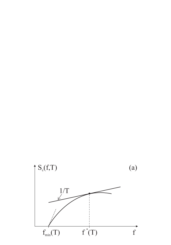
\begin{picture}(11.0,6.5)\centerline{\hbox{\psfig{angle=0,width=312.9803pt}}} \end{picture}

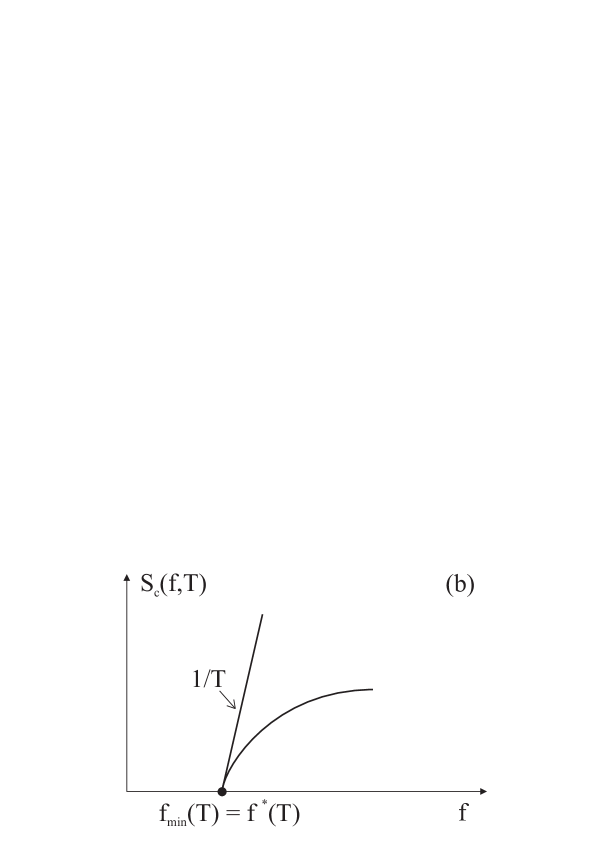
Figure 8: Schematic $f$-dependence of the configurational entropy $S_{c}(f,T)$. (a) $T_{K}<T<T_{c}$ where $f^{*}(T)$ is between $f_{\textrm{min}}(T)$ and $f_{\textrm{max}}(T)$, (b) $T\leq T_{K}$ where $f^{*}(T)$ coincides with $f_{\textrm{min}}(T)$. Note that the slope of the tangent (which must equal $1/T$) in (a) is smaller than in (b). The dashed line in part (a) shows the slope of the tangent at $f_{\textrm{min}}(T)$.

$$s_{0}(T)=\frac{\partial S_{c}}{\partial f}(f_{\textrm{min}}(T),T)<\infty$$ (97)

this will happen at a temperature $T_{s}>0$ with

$$\frac{1}{T_{s}}=s_{0}(T_{s})\quad.$$ (98)

Since $S_{c}$ vanishes at $T_{s}$ it is identical to the Kauzmann temperature $T_{K}$. The reader should note that the existence of a nonzero Kauzmann temperature and accordingly the existence of a static glass transition at $T_{K}$ relies on the finite value of $s_{0}(T)$ for all temperatures, including zero.

Now, it is the major goal to calculate the free energy $\Phi(T)$ and the configurational entropy below $T_{K}$. This can be done by a trick. Instead of taking one system one chooses $m$ replicas which are weakly coupled to each other with coupling constant $\varepsilon$ 49rs ; 50rs ; 51rs . In the glass phase, i.e. below $T_{K}$ this small coupling will force all systems into the same local minimum $\alpha$. Therefore the corresponding partition function is given by:

$$Z_{m}(T,N)\approx\int\limits^{f_{max}(T)}_{f_{min}(T)}df\exp\{-N[m\beta f-S_{c}(f,T)]\}$$ (99)

in analogy to Eq. (92). The “saddle point” condition Eq. (95) is:

$$\frac{m}{T}=\frac{\partial S_{c}}{\partial f}(f,T)\quad.$$ (100)

If we allow $m$ to take any real positive value, it is obvious that Eq.( 100) has a solution $f^{*}_{m}(T)>f_{\textrm{min}}(T)$ if $m<1$ is small enough, even if $f^{*}_{m=1}(T)=f_{\textrm{min}}(T)$. Then the free energy $\Phi(m,T)$ is given by:

$$\Phi(m,T)=\min\limits_{f}[mf-TS_{c}(f,T)]\quad.$$ (101)

Next, it is easy to prove that $\Phi(m,T)$ and the free energy per particle of the replicated system:

$$\phi(m,T)=\frac{1}{m}\Phi(m,T)$$ (102)

allows to calculate $f(T)$ and $S_{c}(T)$:

$$f(T)=\frac{\partial\Phi(m,T)}{\partial m}$$ (103)

$$S_{c}(T)=\frac{m^{2}}{T}\frac{\partial\phi(m,T)}{\partial m}\quad.$$ (104)

Hence, the knowledge of $\Phi(m,T)$ allows to determine $f$ and $S_{c}$. Increasing $m$ towards one there will be a critical value $0\leq m^{*}(T)\leq 1$ at which $f_{m}^{*}(T)=f_{\textrm{min}}(T)$. A schematic representation of the $m-T$ phase diagram is given in Fig. 9. There are two phases: a liquid phase above the solid line. For $T>T_{K}$ it is a liquid where the replicas become uncorrelated for $\varepsilon\rightarrow 0$ whereas for $T<T_{K}$ and $m<m^{*}(T)$ it is “molecular liquid” where the particles of the $m$ replica form “molecules” even for $\varepsilon\rightarrow 0$. Below the solid line there is a glass phase. Since $S_{c}(T)=0$ in the glass phase, Eq. (104) implies that $\phi(m,T)$ is independent on $m$, i.e. it is:

$$\phi(m,T)=\phi(1,T)$$ (105)

for all $m\geq m^{*}(T)$ and $T<T_{K}$. On the other hand $\phi(m,T)$ is continuous at the liquid-glass phase boundary $m^{*}(T)$:

$$\phi_{\textrm{liquid}}(m^{*}(T),T)=\phi_{\textrm{glass}}(m^{*}(T),T)$$ (106)

combining Eq. (105) and Eq. (106) one arrives at the important result:

$$\Phi(T)\equiv\phi(1,T)=\phi_{\textrm{liquid}}(m^{*}(T),T)\quad.$$ (107)

Due to Eq. (107) one can calculate the free energy $\Phi(T)$ of the physical system from the free energy of the replica system in its liquid phase, despite $T<T_{K}$. Since there are powerful techniques for the calculation of the liquid free energy 40rs the relationship Eq. (107) allows to calculate $\Phi(T)$ from $\phi(m,T)$ and the latter also allows to determine the configurational entropy $S_{c}(f,T)$ from Eq. (103) and Eq. (104) by eliminating $m$.

\begin{picture}(11.0,7.0)\centerline{\hbox{\psfig{angle=-90,width=256.0748pt}}} \end{picture}

Figure 9: Phase diagram of the replica system in the m-T-space. Solid line separates the liquid from the glass phase (see also text). The dashed line within the liquid phase separates the “atomic” liquid for $T>T_{K}\simeq 0.5$ from the “molecular” liquid for $T<T_{K}$. The curved part of the solid line is $m^{*}(T)$.

4.2 Microscopic description

In the last section we have shown that the free energy $\Phi(T)$ and the configurational entropy $S_{c}(f,T)$ can be obtained from $\Phi(m,T)$, the free energy of a replica system in its liquid phase. Now we will describe how this can be performed from first principles.

The potential energy of a N-particle system in a volume $V$ may be given by pair potentials $v(\vec{x})$:

$$V(\vec{x}_{1},\ldots,\vec{x}_{N})=\sum\limits_{i<j}v(\vec{x}_{i}-\vec{x}_{j})\quad.$$ (108)

Let us consider $m$ identical systems (replicas) which are weakly coupled by an attractive pair potential $w(\vec{x}_{i}^{a}-\vec{x}_{j}^{b})$, which is considered to be short ranged. Then the total potential energy is given by:

$$V^{\varepsilon}_{m}(\{\vec{x}_{i}^{a}\})=\sum\limits_{a=1}^{m}V(\vec{x}_{1}^{a},\ldots,\vec{x}_{N}^{a})+\varepsilon\sum\limits_{a<b}\sum\limits_{i<j}w(\vec{x}^{a}_{i}-\vec{x}_{j}^{b})$$ (109)

where $\vec{x}_{i}^{a}$ is the position of particle $i$ in replica $a$ and $\varepsilon\geq 0$ is an infinitesimal coupling constant. Note, that $w$ breaks the replica permutational symmetry. It acts like a symmetry breaking magnetic field in case of a ferromagnet. For $\varepsilon>0$ the thermodynamic limit $N\rightarrow\infty$ forces the replicas into the same local minima. Taking the limit $\varepsilon\rightarrow\infty$ afterwards leaves the replicas in the same state for $T<T_{K}$ and makes them uncorrelated for $T>T_{K}$ (cf. discussion in section 4.1). Therefore for $T<T_{K}$ and $\varepsilon>0$ it is (using an appropriate labelling of the particles):

$$\vec{x}_{i}^{1}\approx\vec{x}_{i}^{2}\approx\cdots\approx\vec{x}_{i}^{m}$$ (110)

Therefore we can introduce center of mass coordinates $\vec{X}_{i}$ of an “$m$-atomic molecule” and relative coordinates $\vec{u}_{i}^{a}$ such that

$$\vec{x}_{i}^{a}=\vec{X}_{i}+\vec{u}_{i}^{a}$$ (111)

where

$$\vec{X}_{i}=\frac{1}{m}\sum\limits_{a=1}^{m}\vec{x}_{i}^{a}$$ (112)

and ${\vec{u}_{i}^{a}}$ has to fulfil the $N$ constraints:

$$\sum\limits_{a=1}^{m}\vec{u}_{i}^{a}=0$$ (113)

for all $i$.

The classical partition function (configurational part) is given by:

$$Z^{\varepsilon}_{m}(T,N)=\frac{1}{N!}\int\prod\limits_{i,a}d^{d}x^{a}_{i}\exp[-\beta V^{\varepsilon}_{m}(\{\vec{x}_{i}^{a}\})]$$ (114)

where $d$ is the spatial dimension. Making use of Eq. (111) this leads to

$$Z^{\varepsilon}_{m}(T,N)=\frac{1}{N!}\int\prod\limits_{i}d^{d}X_{i}\int\prod\limits_{i,a}d^{d}u^{a}_{i}$$ (115)

$$\prod\limits^{d}_{i=1}\Big{(}m^{d}\delta\Big{(}\sum\limits_{a}\vec{u}_{i}^{a}\Big{)}\Big{)}\exp[-\beta V^{\varepsilon}_{m}(\{\vec{X}_{i}\},\{\vec{u}_{i}^{a}\})]$$

where the $\delta$-function accounts for the constraints Eq. (113). Due to Eq. (110), it is $|\vec{u}_{i}^{a}|\ll 1$. Therefore a harmonic approximation can be applied which yields:

$$Z^{\varepsilon}_{m}(T,N)=Z_{m}(T,N)\cong\frac{1}{N!}\int\prod\limits_{i}d^{d}X_{i}\int\prod\limits_{i,a}d^{d}u^{a}_{i}\cdot$$

$$\cdot\prod\limits_{i}\Big{(}m^{d}\delta\Big{(}\sum\limits_{a}\vec{u}^{a}_{i}\Big{)}\Big{)}\cdot\exp\Big{\{}-\beta\Big{[}mV(\{\vec{X}_{i}\})+$$

$$+\frac{1}{2}\sum\limits_{a}\sum\limits_{i\mu,j\nu}M_{i\mu,j\nu}(\{\vec{X}_{i}\})(u^{a}_{i\mu}-u^{a}_{j\nu})^{2}\Big{]}\Big{\}}$$ (116)

where $(M_{i\mu,j\nu})$ is the Hessian matrix of V and $\vec{u}^{a}_{i\mu}$ is the $\mu$-component of $\vec{u}^{a}_{i}$. Note that we were allowed to put $\varepsilon=0$, because we already assumed that Eq. (110) holds. Using an integral representation of the $\delta$-function the integral with respect to $\vec{u}^{a}_{i\mu}$ are Gaussian and can be performed which involves

$$\Big{[}\prod\limits^{Nd}_{k=1}\lambda_{k}(\{\vec{X}_{i}\})\Big{]}^{1/2}\Big{[}\prod\limits^{Nd}_{k=1}\lambda_{k}(\{\vec{X}_{i}\})\Big{]}^{-m/2}=\exp\Big{[}-\frac{m-1}{2}\textrm{Tr}\ln(M_{i\mu,j\nu}(\{\vec{X}_{i}\}))\Big{]}$$ (117)

where $\lambda_{k}$ are the eigenvalues of $(M_{i\mu,j\nu})$. The result can be brought into the following form:

$$Z_{m}(T,N)\cong(c_{m}(T))^{N}Z_{1}(T/m,N)\Big{\langle}\exp\Big{[}-\frac{m-1}{2}\textrm{Tr}\ln(M_{i\mu,j\nu}(\{\vec{X}_{i}\}))\Big{]}\Big{\rangle}(T/m)$$ (118)

where:

$$c_{m}(T)=m^{\frac{d}{2}}(2\pi T)^{\frac{d}{2}(m-1)}\quad.$$ (119)

$Z_{1}(T/m,N)$ is the partition function of the original system, but at a temperature $T/m$ and $\langle(\cdot)\rangle$ denotes averaging with respect to $\exp[-\beta mV(\{\vec{X}_{i}\})]/Z_{1}\\ (T/m,N)$. In a next step one uses the approximation:

$$\Big{\langle}\exp\Big{[}\cdots\Big{]}\Big{\rangle}\approx\exp\Big{[}-\frac{m-1}{2}\langle\textrm{Tr}\ln(M_{i\mu,j\nu}(\{\vec{X}_{i}\}))\rangle\Big{]}\quad.$$ (120)

The r.h.s. of Eq. (120) could be calculated if the density distribution of the eigenvalues would be known, which is not the case. Therefore, some more approximations are necessary. We will not present these technical manipulations which can be found in Ref. 50rs but present the idea. Let us skip for a moment the logarithm in Eq. (120). Then we have to calculate $\langle\textrm{Tr}(M_{i\mu,j\nu}(\{\vec{X}_{i}\}))\rangle=\sum\limits_{i,\mu}\langle M_{i\mu,i\mu}(\{\vec{X}_{i}\})\rangle$. Since $M_{i\mu,i\mu}(\{\vec{X}_{i}\})=\sum\limits_{j}(\partial^{2}v/\partial r^{2}_{\mu})(\vec{r}=\vec{X}_{i}-\vec{X}_{j})$ this involves the average of the second derivatives of the pair potential $v(\vec{r})$. Assuming that $M_{i\mu,i\mu}$ do not fluctuate much one obtains finally

$$\langle\textrm{Tr}(M_{i\mu,j\nu}(\{\vec{X}_{i}\}))\rangle\Big{(}\frac{T}{m}\Big{)}\approx\frac{N}{d}\int d^{d}rg\Big{(}\vec{r},\frac{T}{m}\Big{)}\vec{\nabla}^{2}v(\vec{r})$$ (121)

i.e. $\langle\textrm{Tr}(M_{i\mu,j\nu}(\{\vec{X}_{i}\}))]\rangle(T/m)$ can be related to the pair distribution function at $T/m$. In a similar way one can express $\langle\textrm{Tr}\ln(M_{i\mu,j\nu}(\{\vec{X}_{i}\}))]\rangle(T/m)$ by $g(\vec{r},T/m)$:

$$\langle\textrm{Tr}\ln(M_{i\mu,j\nu}(\{\vec{X}_{i}\}))]\rangle\Big{(}\frac{T}{m}\Big{)}\approx N{\cal G}\Big{[}g(\vec{r};\frac{T}{m})\Big{]}\;.$$ (122)

Using these approximations we end up with the free energy $\Phi(m,T)=-T\lim\limits_{N\rightarrow\infty}N^{-1}\ln Z_{m}(T,N)$:

$$\beta\Phi(m,T)\approx-\ln c_{m}(T)+\Phi(T/m)+\frac{1}{2}(m-1){\mathcal{G}}[g(\vec{r};T/m)]\quad.$$ (123)

This result demonstrates what has been discussed in section 4.1. The free energy $\Phi(m,T)$ of the replica system is given by the free energy of the original system $(m=1)$ at $T/m$ and by a functional ${\mathcal{G}}$ of the pair distribution function of the original system, also at $T/m$. In the liquid phase $\Phi(T/m)$ can also be expressed by $g(\vec{r},T/m)$ 40rs . Therefore, up to an irrelevant term $\ln c_{m}(T)$ one has succeeded to express $\Phi(m,T)$ by the pair distribution function at a temperature $T/m$. If $T$ is below $T_{K}$, one has to choose $m$ small enough in order to be in the liquid phase. As already mentioned above there are powerful methods 40rs to calculate $g(\vec{r},T/m)$ for the liquid phase. Finally, the such obtained $\Phi(m,T)$ allows to determine $\Phi(T)$ and $S_{c}(f,T)$ as described in section 4.1. In Figure 10 we show $S_{c}(f,T)$ obtained by Mézard and Parisi 49rs for a three-dimensional system $(d=3)$ with density one and a soft sphere pair potential $v(\vec{r})=|\vec{r}|^{-12}$. The $f-$dependence has the qualitatively correct behavior, on which the discussion in section 4.1 has been founded. Using the condition Eq. (98) for the static glass transition point with $T_{s}\equiv T_{K}$ these authors obtained $T_{K}\cong 0.194$ or $\Gamma_{K}\cong 1.51$ for the dimensionless coupling parameter $\Gamma=nT^{-1/4}$. This value is in a reasonable range and is close to the values $\Gamma_{K}^{sim}\cong 1.60$ 52rs and 1.46 53rs from a MD-simulation of binary soft sphere liquids. Since the authors of Ref. 53rs claim that their results are compatible with MCT, it is not quite obvious whether the numerical values yield $\Gamma_{c}=nT_{c}^{-1/4}$ or not.

\begin{picture}(11.0,7.0)\centerline{\hbox{\psfig{angle=-90,width=256.0748pt}}} \end{picture}

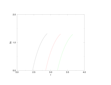
Figure 10: Microscopic result for $S_{c}(f,T)$ for $T=0.05,0.1,0.15$ (from left to right) for a system with soft sphere potential (see also text).

5 SUMMARY

In this article we have reviewed phenomenological and microscopic theories for the structural glass transition. The phenomenological approaches rely on several assumptions which are not proven to be correct. Although they are connected with appealing “physical pictures” their predictive power is limited. However, one class of them has obtained a microscopic justification by the replica theory for structural glasses 45rs ; 49rs ; 50rs . This theory, based on first principles, predicts a static glass transition at the Kauzmann temperature $T_{K}$ where the configurational entropy $S_{c}(T)$ vanishes, as stated in the Adams-Gibbs-theory (1st chapter). Although one can avoid the use of replicas 54rs , the replica theory has a certain beauty because the several equivalent glass phases with same free energy can be described by copying the system $m$ times and introducing a weak coupling between the copies (replicas). This coupling acts as a “symmetry” breaking field similar to a magnetic field for a ferromagnet. Analytically continuing $m$ to positive real numbers allows to relate the thermodynamical properties of the glass phase, i.e. for $T<T_{K}$, to those of the liquid phase, provided $m$ is taken small enough with respect to one.

Quite a different type of transition is obtained from mode coupling theory 27rs ; 28rs ; 29rs . MCT is a dynamical theory, in contrast to replica theory. It provides an equation of motion for, e.g. the spatial Fourier transform $\Phi(\vec{q},t)$ of the normalized density correlator of a simple liquid. Extension to molecular liquids is straightforward 15rs ; 30rs ; 31rs ; 32rs ; 33rs . MCT predicts the existence of a dynamical glass transition at a temperature $T_{c}$ where the dynamics changes qualitatively. Above $T_{c}$ the correlator $\Phi$ decays to zero, and converges to the nonergodicity parameter $f(\vec{q})>0$, below $T_{c}$. The nonergodicity parameters vary discontinuously at $T_{c}$ and can be interpreted as glass order parameters. Besides this, MCT makes several new predictions. Close to $T_{c}$ there exist two scaling laws, the critical and the von Schweidler law. The corresponding time scales $t_{\sigma}(T)$ and $\tau(T)$ exhibit power law divergence at $T_{c}$. For times much larger than a typical microscopic time $t_{0}$ and much smaller than the $\alpha$-relaxation time scale $\tau(T)$ the $\vec{q}$- and $t$-dependence of $\Phi(\vec{q},t)$ factorize, which is a very strong statement. Furthermore, all the exponents of those power laws can be obtained from one parameter $\lambda$, only, the exponent parameter. $\lambda$ is determined by the static correlator $S(\vec{q})$ at $T_{c}$. This proves the very microscopic nature of MCT. Although $\lambda$ and therefore the exponents are dependent on the physical system, i.e. on the interaction, they are universal for all correlators of one system which couple to the density fluctuations 27rs .

These two microscopic theories in some sense are complementary to each other and yield two different glass transition points. It is interesting that the existence of a static and a dynamical glass transition had also been found for mean field spin glasses with discontinuous order parameter. There it has even been speculated that spin glasses are quite similar to structural glasses 8rs . For the mean field spin glasses both transitions are related to singularities and occur at $T_{K}$ and $T_{c}$ with $T_{K}<T_{c}$. Therefore both transitions are sharp. Concerning MCT (as described in the 3rd chapter), sometimes called idealized mode coupling theory, it has been shown 35rs ; 55rs ; 56rs that the singularity is removed, due to ergodicity restoring processes. Nevertheless, if the time scale of these processes is much larger than $\tau(T)$, one can observe in a certain time and temperature window the dynamical behavior as predicted from the idealized theory 27rs ; 28rs ; 29rs . Deviations start to emerge very close to $T_{c}$. This fact has some importance for the static glass transition. For mean field spin glasses it was proven 57rs ; 58rs that the system does not relax to equilibrium below $T_{c}$. Therefore the static transition at $T_{K}$ is masked. Due to the ergodicity restoring processes this is not anymore true for systems with finite range interactions. Despite of that, it is by far not clear that there is a minimum free energy $f_{\textrm{min}}(T)$ at which the configurational entropy $S_{c}(f,T)$ vanishes linearly with a slope $s_{0}(T)=(\partial S_{c}/\partial f)(f_{\textrm{min}}(T),T)<\infty$. This is a very strong assumption which may not be fulfilled in general. For real systems, i.e. in finite dimensions, with short range interactions the physical picture described in section 4.1 probably does not hold, i.e.  there are not an exponential number of states with density $\rho^{(\alpha)}(\bf x)$ and infinite life time. However, there might exist systems with large enough frustration being close to the idealized situation, at least on a finite time scale. The same holds for MCT. For instance, the ergodicity restoring processes seem to be extremely weak for colloidal systems. Indeed it has been shown that the dynamics of colloids can be described over many decades in time by MCT 59rs .

Independent on whether the singularities of both microscopic theories exist or not, the progress which has been made is significant, this is particularly true for MCT. The number of experiments and simulations 12rs ; 13rs ; 14rs ; 15rs (see also the contribution by U. Buchenau in this monograph) having found consistency with the MCT-predictions in an appropriately chosen time and temperature interval is enormous, despite the deviations very close to $T_{c}$. One may hope that the few tests 60rs of replica theory may be continued in order to check its validity in more detail. And an extension including time-dependence would be desirable as well.

Both theories probably describe idealized situations only. As mentioned above MCT has been extended 55rs ; 56rs to include ergodicity restoring processes. But this extended version has not really been tested, because it is rather involved. Describing the ergodicity restoring processes by a single parameter $\delta$ there was a comparison with experimental data which is satisfactory 61rs . Whether replica theory can be extended in case that the singularity is spurious is not clear. Such an extension might also lead to a much more complicated mathematical structure. In that case it might be much better to restrict to the idealized version, which holds for both theories.

Nevertheless there are still many challenging problems left. Let us mention some of them:

• further investigations of similarities and dissimilarities between systems with and without quenched disorder

• glass transition in lattice gas models 62rs

• connection between the “potential energy landscape” properties 16rs ; 17rs ; 18rs with MCT and replica theory; e.g. it has been shown that the saddle index vanishes at the MCT-temperature $T_{c}$ 63rs

• investigation of models with trivial statics which may not exhibit a static glass transition but a MCT-like one 64rs

• investigations of models without or weak static correlations 65rs , where replica theory and MCT (in its present form) do not yield a glass transition, although found in simulations 66rs

• nonequilibrium behavior (aging)

ACKNOWLEDGMENT: I gratefully acknowledge valuable comments on this manuscript by Pablo G. Debenedetti, Wolfgang Götze and Marc Mézard. Figures 9 and  10 were provided by Marc Mézard and Figures 1 and  2 were produced by Michael Ricker. I also would like to thank both for their support.

References

- (1) K. Binder and A. P. Young, Rev. Mod. Phys. 58, 801,(1986)
- (2) M. Mézard, G. Parisi and M. A. Virasoro “Spin Glass Theory and Beyond”, World Scientific, Singapore 1987
- (3) J. Wong and C. A. Angell “Glass: Structure by Spectroscopy”, Dekker, New York, 1976; C. A. Angell, Science 267, 1924 (1995)
- (4) J. Jäckle, Rep. Prog. Phys. 49, 171 (1986)
- (5) P. G. Debenedetti “Metastable Liquids: Concepts and Principles, Princeton University Press, Princeton, 1996
- (6) E. Donth “The Glass Transition: Relaxation Dynamics in Liquids and Disordered Materials”, Material Science, Springer-Verlag, Berlin 2001
- (7) J.-P. Bouchaud and M. Mézard, J. Phys. I (France) 4, 1109 (1984); E. Marinari, G. Parisi and F. Ritort, J. Phys. A27, 7615 (1994); A27, 7647 (1994); L. F. Cugliandolo, J. Kurchan, G. Parisi and F. Ritort, Phys. Rev. Lett. 74, 1012 (1995); P. Chandra, L. B. Ioffe and D. Sherrington, Phys. Rev. Lett. 75, 713 (1995); L. B. Ioffe and A. V. Lopatin, J. Phys.: Condens. Matter 13, L371 (2001)
- (8) T. R. Kirkpatrick and D. Thirumalai, Phys. Rev. Lett. 58, 2091 (1987); Phys. Rev. B36, 5388 (1987); T. R. Kirkpatrick and P. G. Wolynes, Phys. Rev. B36, 8552 (1987)
- (9) A. L. Greer, Nature 404, 134 (2000); F. H. Stillinger and P. G. Debenedetti, Biophysical Chemistry, in press; M. R. Feeney, P. G. Debenedetti and F. H. Stillinger, submitted to J. Chem. Phys.
- (10) F. H. Stillinger, P. G. Debenedetti and T. M. Truskett, J. Phys. Chem. B105, 11809 (2001)
- (11) U. Bengtzelius, W. Götze and A. Sjölander, J. Phys. C17, 5915 (1984)
- (12) W. Götze and L. Sjögren, Rep. Prog. Phys. 55, 241 (1992); W. Götze, J. Phys.: Condens. Matter 11, A1 (1999)
- (13) W. Kob and H. C. Anderson, Transp. Theory Stat. Phys. 24, 1179 (1995); W. Kob in “Experimental and Theoretical Approaches to Supercooled Liquids: Advances and Novel Applications”, eds. J. Fourkas, D. Kivelson, U. Mohanty and K. Nelson, ACS Books, Washington, 1997: p. 28; W. Kob, J. Phys.: Condens. Matter 11, R85 (1999) W. Kob, Les Houches lecture notes 2002, cond-mat/0212344.
- (14) F. Sciortino, P. Gallo, P. Tartaglia and S.-H. Chen, Phys. Rev. E54, 6331 (1996); F. Sciortino, L. Fabbian, S.-H. Chen and P. Tartaglia, Phys. Rev. E56, 5397 (1997); C. Theis, F. Sciortino, A. Latz, R. Schilling and P. Tartaglia, Phys. Rev. E62, 1856 (2000); S. Kämmerer, W. Kob and R. Schilling, Phys. Rev. E56, 5450 (1997); E58, 2131, 2141 (1998); A. Winkler, A. Latz, R. Schilling and C. Theis, Phys. Rev. E62, 8004 (2000)
- (15) L. Fabbian, A. Latz, R. Schilling, F. Sciortino, P. Tartaglia and C. Theis, Phys. Rev. E60, 5768 (1999)
- (16) M. Goldstein, J. Chem. Phys. 51, 3728 (1969); F. H. Stillinger and T. A. Weber, Phys. Rev. A25, 978 (1982); F. H. Stillinger, Science 267, 1935 (1995); D. Sherrington, Physica D107, 117 (1997).
- (17) S. Sastry, P. G. Debenedetti and F. H. Stillinger, Nature 393, 554 (1998); S. Büchner and A. Heuer, Phys. Rev. Lett. 84, 2168 (2000); T. B. Schrøder, S. Sastry, J. C. Dyre and S. C. Glotzer, J. Chem. Phys. 112, 9834 (2000); L. Angelani, R. Di Leonardo, G. Ruocco, A. Scala and F. Sciortino, Phys. Rev. Lett. 85, 5356 (2000); K. Broderix, K. K. Bhattacharya, A. Cavagna, A. Zippelius and I. Giardina, Phys. Rev. Lett. 85, 5360 (2000); A. Cavagna, Europhys. Lett. 53, 490 (2001); T. S. Grigera, A. Cavagna, I. Giardina and G. Parisi, Phys. Rev. Lett. 88, 055502 (2002); J. P. K. Doyle and D. J. Wales, J. Chem. Phys. 116, 3777 (2002)
- (18) F. Sciortino, W. Kob and P. Tartaglia, Phys. Rev. Lett. 83, 3214 (1999)
- (19) G. Adam and J. H. Gibbs, J. Chem. Phys. 43, 139 (1965)
- (20) W. Kauzmann, Chem. Rev. 43, 219 (1948)
- (21) M. H. Cohen and D. Turnbull, J. Chem. Phys. 31, 1164 (1959)
- (22) M. H. Cohen and G. S. Grest, Phys. Rev. B20, 1077 (1979); ibid B24 (1981)
- (23) D. Stauffer and A. Aharony “Introduction to Percolation Theory”, Taylor and Francis Ltd., London, 1994
- (24) J. H. Gibbs, J. Chem. Phys. 25, 185 (1956); J. H. Gibbs and E. A. Di Marzio, J. Chem. Phys. 28, 373 (1958)
- (25) P. J. Flory, J. Chem. Phys. 9, 660 (1941); M. L. Huggins, J. Chem. Phys. 9, 440 (1941)
- (26) K. Kawasaki in “Phase Transitions and Critical Phenomena”, eds. C. Domb and M. S. Green, Academic Press, London, 1976
- (27) W. Götze in “Liquids, Freezing and the Glass Transition”, eds. J. P. Hansen, D. Levesque and J. Zinn-Justin, North Holland, Amsterdam 1991
- (28) R. Schilling in “Disorder Effects on Relaxational Processes”, eds. R. Rickert and A. Blumen, Springer-Verlag, Berlin, 1994
- (29) H. Z. Cummins, J. Phys.: Condens. Matter 11, A95 (1999)
- (30) T. Franosch, M. Fuchs, W. Götze, M. R. Mayr and A. P. Singh, Phys. Rev. E56, 5659 (1997)
- (31) R. Schilling and T. Scheidsteger, Phys. Rev. E56, 2932 (1997); R. Schilling, Phys. Rev. E65, 051206 (2002)
- (32) S.-H. Chong and F. Hirata, Phys. Rev. E58, 6188 (1998)
- (33) S.-H. Chong, W. Götze and A. P. Singh, Phys. Rev. E63, 011206 (2001)
- (34) T. R. Kirkpatrick, Phys. Rev. A31, 939 (1985)
- (35) S. P. Das and G. F. Mazenko, Phys. Rev. A34, 2265 (1986)
- (36) T. R. Kirkpatrick and P. G. Wolynes, Phys. Rev. A35 (1987)
- (37) E. Zaccarelli, G. Foffi, F. Sciortino, P. Tartaglia and K. A. Dawson, Europhys. Lett. 55, 157 (2001)
- (38) S. Franz and J. Hertz, Phys. Rev. Lett. 74, 2114 (1995)
- (39) J.-P. Bouchaud, L. F. Cugliandolo, J. Kurchan and M. Mézard, Physica A226, 243 (1996)
- (40) J. P. Hansen and I. R. McDonald “Theory of Simple Liquids”, 2nd edition, Academic Press, London, 1986
- (41) D. Forster “Hydrodynamical Fluctuations, Broken Symmetry and Correlation Functions", Benjamin, Reading, 1975
- (42) F. Sciortino and W. Kob, Phys. Rev. Lett. 86, 648 (2001)
- (43) W. Götze, Z. Phys. B56, 139 (1984)
- (44) W. Götze, Z. Phys. B60, 195 (1985)
- (45) M. Mézard and G. Parisi, J. Phys. A29, 6515 (1996)
- (46) Y. Singh, J. P. Stoessel and P. G. Wolynes, Phys. Rev. Lett. 54, 1059 (1985)
- (47) N. D. Mermin, Phys. Rev. 137, A 1441 (1965)
- (48) T. V. Ramakrishnan and M. Youssouff, Phys. Rev. B19, 2775 (1979)
- (49) M. Mézard and G. Parisi, Phys. Rev. Lett. 82, 747 (1999)
- (50) M. Mézard and G. Parisi, J. Chem. Phys. 111, 1076 (1999)
- (51) R. Monasson, Phys. Rev. Lett. 75, 2847 (1995); S. Franz and G. Parisi, J. Phys. I, (France) 5, 1401 (1995)
- (52) B. Bernu, Y. Hiwatari and J. P. Hansen, J. Phys. C18, L371 (1985)
- (53) J. N. Roux, J. L. Barrat and J. P. Hansen, J. Phys.: Condens. Matter 1, 7171 (1989)
- (54) M. Mézard and G. Parisi, J. Phys.: Condens. Matter 12, 6655 (2000)
- (55) W. Götze and L. Sjögren, Z. Phys. B.65, 415 (1987)
- (56) R. Schmitz, J. W. Dufty and P. De, Phys. Rev. Lett. 71, 2066 (1993)
- (57) H. Horner, Z. Phys. B66, 175 81987); A. Crisanti, H. Horner and H. J. Sommers, Z. Phys. B92, 257 (1993)
- (58) L. F. Cugliandolo and J. Kurchan, Phys. Rev. Lett. 71, 173 (1993)
- (59) W. van Megen and S. M. Underwood, Phys. Rev. E47, 248 (1993)
- (60) B. Coluzzi, M. Mézard, G. Parisi and P. Verrocchio, J. Chem. Phys. 111, 9039 (1999); B. Coluzzi, G. Parisi and P. Verrocchio, J. Chem. Phys. 112, 2933 (2000); B. Coluzzi, G. Parisi and P. Verrocchio, Phys. Rev. Lett. 84, 306 (2000)
- (61) H. Z. Cumnmins, W. M. Du, M. Fuchs, W. Götze, S. Hildebrand, A. Latz, G. Li and N. J. Tao, Phys. Rev. E47, 4223 (1993)
- (62) W. Kob and H. C. Andersen, Phys. Rev. E48, 4364 (1993); G. Biroli and M. Mézard, Phys. Rev. Lett. 88, 025501 (2002); A. Lawlor, D. Reagan, G. D. McCullagh, P. De Gregorio, P. Tartaglia and K. A. Dawson, Phys. Rev. Lett. 89, 245503 (2002)
- (63) L. Angelani et al., K. Broderix et al. and T. S. Grigera et al. from Ref. 17rs
- (64) K. Kawasaki and B. Kim, Phys. Rev. Lett. 86, 3582 (2001); K. Kawasaki and B. Kim, J. Phys.: Condens. Matter 14, 2265 (2002)
- (65) R. Schilling and G. Szamel, Europhys. Lett. 61, 207 (2003); J. Phys.: Condens. Matter 15, S967 (2003)
- (66) C. Renner, H. Löwen and J. L. Barrat, Phys. Rev. E52, 5091 (1995); S. P. Obukhov, D. Kobsev, D. Perchak and M. Rubinstein, J. Phys. I (France) 7, 563 (1997)
Index
- Adam-Gibbs theory §2.1
- aging item (vi)
- arbitrary molecules §3
- bifurcation scenario §3.2
- calorimetric glass transition §1
- colloidal systems §5
- configurational entropy item 3), §2.4, §4, §5
- convolution approximation §3.1
- correlation scale §3.2
- critical amplitude §3.2
- critical correlator §3.2
- critical law §3.2, §3.2
- critical temperature §3.2
- current density §3.1
- density functional theory §3, §4
- direct correlation function §3.1
- dynamically cooperative regions §2.1
- ergodic §3.2
- ergodicity restoring processes §5
- excess entropy §1
- exponent parameter §3.2, §5
- free energy §4.1, §4.2
- free energy functional §4.1
- free volume item 1)
- free volume theory §2.3
- generalized fluctuating hydrodynamics §3
- glass order parameters §3.2
- harmonic approximation §4.2
- Hessian matrix §4.2
- higher order bifurcation §3.2
- idealized mode coupling theory §5
- intermediate scattering function §3, §3.1
- Kauzmann temperature §1, item 4), §2.4, §4, §4.1, §5
- lattice gas models item (ii)
- linear molecules §3
- longitudinal current density §3.1
- MCT-approximation §3.1
- memory kernel §3.1
- microscopic density §3.1
- microscopic frequencies §3.1
- mode coupling equations §3.1
- mode coupling theory §1, §3, §5
- molecular liquid §4.1
- Mori-Zwanzig projection formalism §3.1
- nonequilibrium item (vi)
- nonergodic §3.2
- nonergodicity parameter §1, §3.2, §5
- one-step replica symmetry breaking §4
- order-disorder transitions §1
- p-spin models §1
- pair distribution function §4.2
- percolation §2.3
- percolation cluster §2.3
- potential energy landscape §1, item (iii)
- Potts glass §1
- reduced Liouvillian §3.1
- replica permutational symmetry §4.2
- replica theory §4, §5
- replicas §4.1, §4.2, §5
- saddle index item (iii)
- scale invariance §3.2
- schematic model §3.2
- separation parameter §3.2
- site-site representation §3
- slow variable §3.1
- spherical model §3
- spin glass models §1, §3
- spin glass transitions §1
- spin glasses §5
- static structure factor §3.1
- structural glass transitions §1
- structural glasses §5
- structural relaxation §3.2
- symmetry breaking field §5
- tensorial formalism §3
- time-temperature superposition principle §3.2
- type-A transition §3.2
- type-B transition §3.2
- vertex §3.1
- vertices §3.1
- Vogel-Fulcher-Tammann law §1, §2.1, §2.2
- von Schweidler law §3.2
- -relaxation §3.2