Minimal model for beta relaxation in viscous liquids

Abstract

Contrasts between beta relaxation in equilibrium viscous liquids and glasses are rationalized in terms of a double-well potential model with structure-dependent asymmetry, assuming structure is described by a single order parameter. The model is tested for tripropylene glycol where it accounts for the hysteresis of the dielectric beta loss peak frequency and magnitude during cooling and reheating through the glass transition.

Viscous liquids approaching the calorimetric glass transition have extremely long relaxation times viscliq . The main relaxation is termed the alpha relaxation. There is usually an additional minor “beta” process at higher frequencies. Dielectric relaxation is a standard method for probing liquid dynamics diel . The study of dielectric beta relaxation in simple viscous liquids was pioneered by Johari and Goldstein more than 30 years ago joh70 ; joh85 , but the origin of beta relaxation is still disputed kah97 ; wag98 ; joh02a . It is unknown whether every molecule contributes to the relaxation all or only those within “islands of mobility” gol69 ; joh76 ; kop00 . Similarly, it is not known whether small angle jumps all ; kau90 ; vog00 or large angle jumps arb96 are responsible for the beta process.

Improvements of experimental techniques have recently lead to several new findings. The suggestion ols98 ; leo99 ; wag99 that the excess wing of the alpha relaxation usually found at high frequencies is due to an underlying low-frequency beta process was confirmed by long time annealing experiments by Lunkenheimer and coworkers lunken (an alternative view is that the wing is a non-beta type relaxation process paluch ). This lead to a simple picture of the alpha process: Once the effect of interfering beta relaxation is eliminated, alpha relaxation obeys time-temperature superposition with a high frequency loss $\propto\omega^{-1/2}$ ols01 . Moreover, it now appears likely that all liquids have one or more beta relaxations lunken ; han97 ; kud97 ; joh02b : Liquids like propylene carbonate, glycerol, salol, and toluene are now known to possess beta relaxation, while o-terphenyl, previously thought to have a beta process only in the glassy state, has one in the equilibrium liquid phase as well. Finally, it has been shown that beta relaxation in the equilibrium liquid does not behave as expected by extrapolation from the glassy phase: In some cases the beta loss peak frequency is temperature independent in the liquid phase (e.g., sorbitol ols98 ), in other cases it is very weakly temperature dependent. On the other hand, the beta relaxation strength always increases strongly with temperature in the liquid phase ols00 ; note1 .

The contrasts between beta relaxation in liquid and glass are clear from Fig. 1(a) which shows beta loss peak frequency and maximum loss for tripropylene glycol cooled through the glass transition and subsequently reheated note2 .

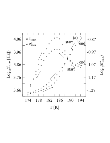
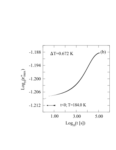
Figure 1: Data for tripropylene glycol. (a) Observation of beta loss peak frequency ($\square$) and loss peak maximum ($\Diamond$) for a continuous passage through the glass transition starting from the equilibrium viscous liquid at 192 K, cooling to 174 K, and reheating to 194 K. After each temperature step the systems is kept at constant temperature for 50 min whereafter a spectrum is measured (sampling time: 6 min). In the glassy phase one observes the well-known strongly temperature-dependent loss peak frequency and weakly temperature-dependent maximum loss; in the liquid phase the situation is the opposite (as seen also in other liquids, e.g., sorbitol ols98 ; ols00 ). There is even a reversal so that the loss peak frequency decreases with increasing temperature. (b) Beta loss peak maximum monitored after a temperature increase of 0.672 K starting from equilibrium at 184.0 K. After 6 s temperature is stable within 1 mK of the final temperature.

In the glassy phase (at low temperatures) the loss peak frequency is strongly temperature dependent while the maximum loss varies little. On the other hand, the loss is strongly temperature dependent in the equilibrium liquid phase. Here we even see the loss peak frequency decreasing upon heating. How is one to understand these findings? A clue is provided by Fig. 1(b) which shows the maximum loss as a function of time after an “instantaneous” temperature step, i.e., instantaneous on the time scale of structural (alpha) relaxation. This experiment utilizes a special-purpose setup with a cell consisting of two aluminum discs separated by three capton spacers (layer distance $\sim\rm 20\mu$, empty capacitance 30 pF). One disc, where temperature is measured via an NTC resistor, is placed on a Peltier element. Less than six seconds after a 0.672 K temperature jump is initiated, temperature is stable within 1 mK. In this setup we measure at 10 kHz which is the loss peak frequency (changes of loss peak frequency lead only to second order corrections of $\epsilon^{\prime\prime}_{\rm max}$). The sampling time is 2 s. Figure 1(b) shows a very fast change of the maximum loss, followed by relaxation toward the equilibrium value taking place on the structural (alpha) relaxation time scale. The existence of an instantaneous increase of the loss clearly indicates a pronounced asymmetry of the relaxing entity. Inspired by this fact we adopt the standard asymmetric double-well potential model (Fig. 2) with transitions between the two free energy minima described by rate theory diel ; glref ; pol72 ; gil81 ; buc01 .

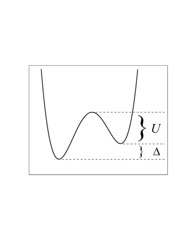
Figure 2: Asymmetric double well potential as a simple model for beta relaxation. The two free energy differences $U$ and $\Delta$ vary as structure changes with temperature in the equilibrium liquid phase, but freeze at the glass transition. Working from this picture the simplest possible assumptions are that 1) Structure is parameterized by just one order parameter, and 2) first order Taylor expansions apply in the relatively narrow temperature range studied.

In terms of the small barrier $U$ and the asymmetry $\Delta$, loss peak frequency $f_{\rm max}$ and maximum loss $\epsilon^{\prime\prime}_{\rm max}$ are given gil81 by

$$\left\{\begin{array}[]{ccl}f_{\rm max}&=&f_{0}\ \displaystyle\exp\left(-\frac{2U+\Delta}{2k_{B}T}\right)\ \cosh\left(\frac{\Delta}{2k_{B}T}\right)\\ \epsilon^{\prime\prime}_{\rm max}&=&\epsilon^{\prime\prime}_{0}(T)\ \displaystyle\cosh^{-2}\left(\frac{\Delta}{2k_{B}T}\right)\end{array}\right.\ \ .$$ (1)

The prefactor $f_{0}$ is assumed to be structure and temperature independent while $\epsilon^{\prime\prime}_{0}(T)\propto 1/T$ gil81 is assumed to be structure independent: $\epsilon^{\prime\prime}_{0}(T)=T_{0}/T$. The free energy differences $U$ and $\Delta$ are expected to change with changing structure, but freeze at the glass transition. In terms of the fictive temperature $T_{f}$ our model is based on

$$\left\{\begin{array}[]{ccccc}U&=&U_{0}&+&a\,k_{B}T_{f}\\ \Delta&=&\Delta_{0}&-&b\,k_{B}T_{f}\end{array}\right.\ \ .$$ (2)

Equation (2) follows from minimal assumptions: Suppose structure is parameterized by just one variable, $s$. Only a rather narrow range of temperatures is involved in studies of beta relaxation in the liquid phase and around the glass transition. Consequently, structure varies only little and, e.g., $U(s)$ may be expanded to first order: $U(s)=c_{0}+c_{1}(s-s_{0})$. For the equilibrium liquid, $s=s(T)$ which may also be expanded to first order. By redefining $s$ via a linear transformation we obtain $s=T$ at equilibrium while $U(s)$ is still linear in $s$. A single variable describing structure, which at equilibrium is equal to temperature, is – consistent with Tool’s 1946 definition too46 – to be identified with the fictive temperature: $s=T_{f}$. Thus one is lead to Eq. (2) where signs are chosen simply to ensure $a,b>0$ in fit to data.

The model has 6 parameters: $f_{0}$, $T_{0}$, $U_{0}$, $\Delta_{0}$, $a$, and $b$. These were determined by measuring the instantaneous changes of $f_{\rm max}$ and $\epsilon^{\prime\prime}_{\rm max}$ upon a temperature step, as well as their thermal equilibrium changes. Figure 1(b) allows determination of the instantaneous change of the loss. It is not possible to determine the instantaneous change of $f_{\rm max}$. Instead we extrapolated measurements obtained by the standard cell note2 as follows (Fig. 3): Beta loss is monitored by first annealing at 183.0 K, subsequently changing temperature to 181.0 K. The latter data show a linear relation between $\log f_{\rm max}$ and $\log\epsilon^{\prime\prime}_{\rm max}$ which, knowing the instantaneous change per Kelvin of $\epsilon^{\prime\prime}_{\rm max}$ from Fig. 1(b), is extrapolated to short times.

In the data analysis it is convenient to eliminate $\cosh$ by introducing the variable

$$Y\ \equiv\ \left(\frac{f_{\rm max}}{f_{0}}\right)^{2}\ \left(\frac{\epsilon^{\prime\prime}_{\rm max}}{\epsilon^{\prime\prime}_{0}(T)}\right)\,.$$ (3)

On the fast time scale $U$ and $\Delta$ are frozen so Eq. (1) implies

$$\left\{\begin{array}[]{ccc}\displaystyle\left.\frac{d\ln Y}{d\ln T}\right|_{\rm inst}&=&\displaystyle\frac{2U+\Delta}{k_{B}T}\\ \displaystyle\left.\frac{d\ln\epsilon^{\prime\prime}_{\rm max}}{d\ln T}\right|_{\rm inst}&=&\displaystyle\frac{\Delta}{k_{B}T}\ \sqrt{1-\frac{\epsilon^{\prime\prime}_{\rm max}}{\epsilon^{\prime\prime}_{0}(T)}}\ -\ 1\end{array}\right.\ \ .$$ (4)

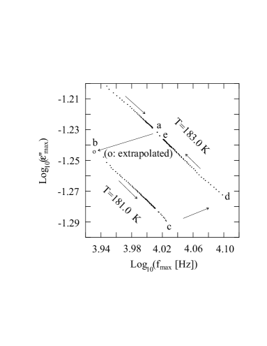
Figure 3: Reversible temperature jump experiment for tripropylene glycol monitoring beta loss peak frequency and loss peak maximum. Starting at 185.0 K (not shown) temperature is first lowered to 183.0 K and kept there for 60 h; the last point, a, was obtained after further 24 h. Then temperature is changed to 181.0 K where it is kept constant for 140 h (initially 20 min between measurements, later 12 hours). The point b is found by extrapolating to zero time after the quench utilizing the data of Fig. 1(b). This series ends at point c, thereafter temperature is changed back to 183.0 K where it is kept for 140 h (all points except the final point e refer to times up to 70 h; e was measured after further 70 h). Equilibrium at 183.0 K is somewhere between points a and e.

Having determined the instantaneous changes of $\epsilon^{\prime\prime}_{\rm max}$ and $f_{\rm max}$, Eqs. (1) and (4) provide 4 equations for the 6 model parameters. The last two equations come from the temperature dependence of loss and loss peak frequency at thermal equilibrium where $U(T)$ and $\Delta(T)$ are given by Eq. (2) with $T_{f}=T$, leading to

$$\left\{\begin{array}[]{ccc}\displaystyle\left.\frac{d\ln Y}{d\ln T}\right|_{\rm eq}&=&\displaystyle\frac{2U_{0}+\Delta_{0}}{k_{B}T}\\ \displaystyle\left.\frac{d\ln\epsilon^{\prime\prime}_{\rm max}}{d\ln T}\right|_{\rm eq}&=&\displaystyle\frac{\Delta_{0}}{k_{B}T}\ \sqrt{1-\frac{\epsilon^{\prime\prime}_{\rm max}}{\epsilon^{\prime\prime}_{0}(T)}}\ -\ 1\end{array}\right.\ \ .$$ (5)

Using Eq. (4) for the data of Figs. 1(b) and 3, and using Eqs. (1) and (5) for equilibrium state measurements at 183 and 185 K, the 6 parameters determined for tripropylene glycol note3 are: $f_{0}=6.2\cdot 10^{11}$ Hz, $T_{0}=130$ K, $U_{0}/k_{B}=-1107$ K, $\Delta_{0}/k_{B}=3039$ K, $a=23.28$, $b=12.77$. $U_{0}<0$ reflects the fact that the beta loss peak frequency in the liquid phase decreases as temperature increases [Fig. 1(a)]. Physically, this anomalous behavior is caused by the barrier $U$ increasing more than $T$ upon heating.

Once all parameters are fixed the model predicts how $f_{\rm max}$ and $\epsilon^{\prime\prime}_{\rm max}$ correlate for the continuous passage through the glass transition of Fig. 1(a). To analyze these data within the model we first note that if $y(x)=1/\cosh^{2}(x)$ then $x=\phi(y)$ where $\phi(y)=\ln(1/\sqrt{y}+\sqrt{1/y-1})$, so Eq. (1) may be inverted: $\Delta/2k_{B}T=\phi(\epsilon^{\prime\prime}_{\rm max}/\epsilon^{\prime\prime}_{0}(T))\equiv\Phi$. Since $\ln Y=-(2U+\Delta)/k_{B}T$ both $\Phi$ and $\ln Y$ involve fictive temperature, and consequently both exhibit hysteresis at the glass transition. However, fictive temperature is eliminated by considering the following variable

$$Z(f_{\rm max},\epsilon^{\prime\prime}_{\rm max})\ \equiv\ \Big{(}2a-b\Big{)}\Phi-\frac{b}{2}\ln\ Y$$ (6)

$$= \ \frac{a\ \Delta_{0}\ +\ b\ U_{0}}{k_{B}T}\ \ .$$

The model is tested in Fig. 4. The glass transition is not visible and most hysteresis is eliminated (better elimination was obtained in Ref. ols00 but without theoretical basis and with one free parameter note4 ). The line shown is the prediction of Eq. (6).

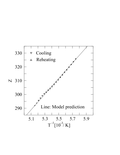
Figure 4: Data for tripropylene glycol from Fig. 1(a) replotted to test the model. The variable $Z$ defined in Eq. (6) is calculated using parameters obtained by independent experiments.

In conclusion, a minimal model for beta relaxation in viscous liquids has been proposed. The model is built on the four simplest possible assumptions: 1) Beta relaxation involves only two levels, 2) structure is determined by just one order-parameter, 3) first order Taylor expansions apply, 4) the two characteristic free energies $U$ and $\Delta$ freeze at the glass transition. The model is clearly oversimplified. For instance, it predicts a Debye response which is not observed, and $U$ and $\Delta$ would be expected to vary slightly with temperature in the glass. Nevertheless, the model is able to rationalize the contrasts between beta relaxation in liquids and in glasses. One final puzzling observation should be mentioned: The asymmetry $\Delta$ extrapolates to zero at a temperature which is close to the temperature where alpha and beta relaxations merge. We have seen the same phenomenon in sorbitol, a pyridine-toluene solution, polypropylene-glycol-425, and in 4,7,10-trioxydecane-1,13-diamine ols98 ; ols00 , and have found no exceptions. This finding indicates that the merging temperature is fundamental, a symmetry is somehow broken below this temperature.

- (1) W. Kauzmann, Chem. Rev. 43, 219 (1948); M. Goldstein, in Modern Aspects of the Vitreous State, edited by J. D. Mackenzie (Butterworths Scientific, London, 1964), p. 90; G. Harrison, The Dynamic Properties of Supercooled Liquids (Academic, New York, 1976); S. Brawer, Relaxation in Viscous Liquids and Glasses (American Ceramic Society, Columbus, OH, 1985); C. A. Angell, K. L. Ngai, G. B. McKenna, P. F. McMillan, and S. W. Martin, J. Appl. Phys. 88, 3113 (2000).
- (2) N. G. McCrum, B. E. Read, and G. Williams, Anelastic and Dielectric Effects in Polymeric Solids (Wiley, New York, 1967); C. J. F. Böttcher and P. Bordewijk, Theory of Electric Polarization, Vol. II: Dielectric Polarization (Elsevier, Amsterdam, 1978); G. Williams, Chem. Soc. Rev. 7, 89 (1978); S. Jr. Havriliak and S. J. Havriliak, Dielectric and Mechanical Relaxation in Materials: Analysis, Interpretation, and Application to Polymers (Hanser Gardner Publ., Munich, 1997).
- (3) G. P. Johari and M. Goldstein, J. Phys. Chem. 74, 2034 (1970); J. Chem. Phys. 53, 2372 (1970).
- (4) G. P. Johari, J. Chim. Phys. 82, 283 (1985).
- (5) S. Kahle, J. Korus, E. Hempel, R. Unger, S. Höring, K. Schröter, and E. Donth, Macromolecules 30, 7214 (1997).
- (6) H. Wagner and R. Richert, J. Phys. Chem. B 103, 4071 (1999).
- (7) G. P. Johari, J. Non-Cryst. Solids 307-310, 317 (2002).
- (8) G. Williams and D. C. Watts, Trans. Faraday Soc. 67, 1971 (1971); C. Hansen and R. Richert, J. Phys.: Condens. Matter 9, 9661 (1997); M. Vogel, C. Tschirwitz, G. Schneider, C. Koplin, P. Medick, and E. Rössler, J. Non-Cryst. Solids 307-310, 326 (2002).
- (9) M. Goldstein, J. Chem. Phys. 51, 3728 (1969).
- (10) G. P. Johari, Annals N. Y. Acad. Sci. 279, 117 (1976).
- (11) J. Köplinger, G. Kasper, and S. Hunklinger, J. Chem. Phys. 113, 4701 (2000).
- (12) S. Kaufmann, S. Wefing, D. Schaefer, and H. W. Spiess, J. Chem. Phys. 93, 197 (1990).
- (13) M. Vogel and E. Rössler, J. Phys. Chem. B 104, 4285 (2000).
- (14) A. Arbe, D. Richter, J. Colmenero, and B. Farago, Phys. Rev. E 54, 3853 (1996).
- (15) N. B. Olsen, J. Non-Cryst. Solids 235-237, 399 (1998).
- (16) C. Leon, K. L. Ngai, and C. M. Roland, J. Chem Phys. 110, 11585 (1999).
- (17) H. Wagner and R. Richert, J. Chem. Phys. 110, 11660 (1999).
- (18) U. Schneider, R. Brand, P. Lunkenheimer, and A. Loidl, Phys. Rev. Lett. 84, 5560 (2000); P. Lunkenheimer, R. Wehn, T. Riegger, and A. Loidl, J. Non-Cryst. Solids 307-310, 336 (2002); P. Lunkenheimer and A. Loidl, Chem. Phys. 284, 205 (2002).
- (19) J. Wiedersich, T. Blochowicz, S. Benkhof, A. Kudlik, N. V. Surovtsev, C. Tschirwitz, V. N. Novikov, and E. Rössler, J. Phys. – Cond. Matter 11, 147 (1999); S. Hensel-Bielowka and M. Paluch, Phys. Rev. Lett. 89, 025704 (2002); A. Doss, M. Paluch, H. Sillescu, and G. Hinze, J. Chem. Phys. 117, 6582 (2002).
- (20) N. B. Olsen, T. Christensen, and J. C. Dyre, Phys. Rev. Lett. 86, 1271 (2001).
- (21) C. Hansen and R. Richert, Acta Polym. 48, 484 (1997).
- (22) A. Kudlik, C. Tschirwitz, S. Benkhof, T. Blochowicz, and E. Rössler, Europhys. Lett. 40, 649 (1997).
- (23) G. P. Johari, G. Power, and J. K. Vij, J. Chem. Phys. 117, 1714 (2002).
- (24) N. B. Olsen, T. Christensen, and J. C. Dyre, Phys. Rev. E 62, 4435 (2000).
- (25) This explains the apparent paradox that in some cases annealing below the glass transition brings out an otherwise invisible beta peak, while in other cases annealing makes the beta peak disappear: If is above the temperature where alpha and beta peaks merge in the equilibrium liquid phase no beta peak is visible in the liquid, and only annealing will bring out the beta peak. On the other hand, if is below the merging temperature the beta peak is visible in the liquid and its magnitude is more or less frozen at the glass transition. In this case, however, annealing below decreases the magnitude of the beta peak because the equilibrium magnitude is strongly temperature dependent. Sometimes the magnitude decreases so much upon annealing that the beta process eventually ends up below the resolution limit.
- (26) The experimental set-up is identical to that used in Ref. ols00 , except for an improved non-commercial 14-bit cosine-wave generator at 16 fixed frequencies per decade used for frequencies below 100 Hz. To eliminate the influence from the high frequency alpha tail the data were subjected to the following procedure: First we obtained the equilibrium shape of the beta peak by annealing for 100 h at 184 K. Then, assuming invariance of the shape of the beta peak, the alpha tail influence was eliminated by subtracting a term ols01 with constant of proportionality adjusted to obtain the invariant shape of the beta peak. This procedure is unique. The subtraction procedure mainly affects and only influences measurements at the highest temperatures. The observed hysteresis effects are much larger than the corrections from subtracting the alpha tail ols00 .
- (27) P. Debye, Polar Molecules (Dover, New York, 1945); H. Fröhlich, Theory of Dielectrics (Oxford University, Oxford, 1949).
- (28) M. Pollak and G. E. Pike, Phys. Rev. Lett. 28, 1449 (1972).
- (29) K. S. Gilroy and W. A. Phillips, Philos. Mag. B 43, 735 (1981); note that in Eq. (1) of this paper should be replaced by .
- (30) U. Buchenau, Phys. Rev. B 63, 104203 (2001).
- (31) A. Q. Tool, J. Am. Ceram. Soc. 29, 240 (1946).
- (32) The parameters were found as follows (note that there is a much larger uncertainty than signaled by the number of digits given): The reference temperature chosen is K. Fitting the data of Fig. 1(b) with a stretched exponential it is possible to extrapolate to zero time - this gives a zero time loss maximum equal to . From this we get . Combining the second halves of Eq. (1) and Eq. (4) we find a transcendental equation for , the solution of which is 3.8414, leading to K. From this and Eq. (1) we can now determine the value of the max loss prefactor, leading to K. Now, taking the last point of Fig. 1(b), where , as representing equilibrium at K, we find . From this the latter of Eq. (5) gives us , leading to K. Knowing both and we find . Using the extrapolation procedure described in the paper, the point b of Fig. 3 is determined; the point b has while the point a has has . This gives us . Finally, to get the equilibrium derivative of we use data not shown in the figures: At K we measure while the point right between the points a and e of Fig. 3, representing equilibrium, tells us that the equilibrium value of at K is given by . This leads to . (The fact that not all derivatives refer to identical temperatures introduces a further element of uncertainty into the parameter estimation.) We are now able to determine the parameter because is the difference between instantaneous and equilibrium ln-ln-derivatives of . This leads to . Moreover, the equilibrium ln-ln-derivative of [Eq. (5)] makes it possible to determine that K. Finally, Eq. (1) at 183 K, the reference temperature, makes it possible to determine the prefactor: Hz.
- (33) Whenever the present model predicts the empirical relation reported in Ref. [24] with .