Development of a density inversion
in driven Granular Gases

Summary.

Granular materials fluidized by a rapidly vibrating bottom plate often develop a fascinating density inversion: a heavier layer of granulate supported by a lower-density region. We employ the Navier-Stokes granular hydrodynamics to follow a density inversion as it develops in time. Assuming a dilute low-Mach-number flow, we derive a reduced time-dependent model of the late stage of the dynamics. The model looks especially simple in the Lagrangian coordinates. The time-dependent solution describes the growth of a density peak at an intermediate height. A transient temperature minimum is predicted to develop in the region of the density peak. The temperature minimum disappears at later times, as the system approaches the steady state. At late times, the predictions of the low-Mach-number model are in good agreement with a numerical solution of the full hydrodynamic equations. At an early stage of the dynamics, pressure oscillations are predicted.

1 Introduction

An ensemble of hard spheres in motion, that collide inelastically and are characterized by a constant coefficient of normal restitution, represents the simplest model of granular gas [1]. It also provides an excellent example of complexity. Indeed, the properties of the granular gas as a whole, such as clustering [2, 3, 4, 5], come out as non-trivial consequences of the simple algebraic laws that govern the velocities of the binary collisions of individual particles. Furthermore, being intrinsically far from thermal equilibrium, granular gas defies statistical mechanics, the cornerstone of the equilibrium science. As the result, formulating a universally applicable continuum theory of granular gas, even in the dilute limit, is not a simple task [6, 7]. The use of the Boltzmann (or Enskog) equation, the starting point of a systematic derivation of the constitutive relations, is based on the Molecular Chaos hypothesis. This hypothesis is justified, in the dilute limit, for an ensemble of elastic hard spheres. Its use for inelastic hard spheres is, rigorously speaking, an uncontrolled assumption. Indeed, inelasticity of the particle collisions introduces inter-particle correlations which can invalidate the Molecular Chaos hypothesis. The correlations become more pronounced as the inelasticity of the collision increases. On the contrary, for nearly elastic collisions, $1-r^{2}\ll 1$ (where $r$ is the coefficient of normal restitution) the correlations are small, and the Boltzmann equation can be used safely (again, in the dilute limit).

An additional crucial assumption, made in the process of the derivation of the hydrodynamics from the Boltzmann equation, is scale separation. The hydrodynamics is valid if the mean free path of the particles is much less than any characteristic length scale, and the mean time between two consecutive collisions is much less than any characteristic time scale, described hydrodynamically. This assumption (as well as the dilute gas assumption, if used) should be verified, in every specific system, after the hydrodynamic problem is solved and the characteristic length and time scales determined. One more criterion for the validity of granular hydrodynamics is the smallness of fluctuations, driven by the noise caused by the discrete nature of the particles. The accuracy of hydrodynamics improves with an increase of the total number of particles in the system $N$ [8].

Once hydrodynamics is valid, it is highly rewarding using it. Hydrodynamics has a great predictive power and helps to identify important collective phenomena (shear flows and vortices, shocks, different modes of clustering flows, phase separation etc.) that are impossible to perceive in the language of individual particles. Once identified, these collective phenomena can then be investigated in experiment and simulations in more general (not necessarily hydrodynamic) formulations. A recent example: employing a variant of granular hydrodynamics, Livne et al. [9] predicted a novel phase separation instability in a system of inelastic hard spheres, driven by a rapidly vibrating plate at zero gravity. This system had been investigated earlier by many workers. However, the phase separation instability, and a plethora of interesting effects accompanying it, were overlooked. Undoubtedly, the reason for that was that hydrodynamics had not been fully appreciated and exploited [10].

In this paper we employ the Navier-Stokes granular hydrodynamics for a theoretical analysis of the process of formation of a density inversion in a dilute granular gas driven by a rapidly vibrating bottom plate in a gravity field. The phenomenon of a density inversion in the steady state of this system is well known in the granular community. On the contrary, the dynamics of the formation of the density inversion has never been investigated previously. As we will see, this dynamics is quite instructive. The hydrodynamic theory yields predictions of time-dependent quantities that can be checked in molecular dynamics simulations and experiment. Our additional motivation here is pedagogical. While dealing with this problem, we will present two useful hydrodynamic techniques. The first is reduction of the order of the hydrodynamic equations, based on a hierarchy of the length/time scales in the problem. The second technique is the use of the Lagrangian coordinates.

Here is a layout of the remainder of this paper. In Sec. 2 we will write down a set of hydrodynamic equations and boundary conditions that describe the dynamics of formation of a density inversion. By introducing scaled variables, we will delineate the two scaled governing parameters of the problem. In Sec. 3 we briefly review the properties of the steady state and the condition for a density inversion. In Sec. 4 we assume a low-Mach-number flow, derive a reduced hydrodynamic model and use it for an investigation of the late-time dynamics of the formation of the density inversion. Section 5 reports a numerical solution of the full hydrodynamic equations and compares the numerical results with the predictions of the low-Mach-number model. A discussion of the results is presented in Sec. 6.

2 The model problem and hydrodynamic equations

We will adopt the simplest possible model, in two dimensions, that exhibits a density inversion. Let $N\gg 1$ identical nearly elastic hard disks of diameter $d$ and mass $m=1$ move without friction in a two-dimensional box of width $L_{x}$ and infinite height. The driving base is at $y=0$, the side walls are at $x=0$ and $x=L_{x}$. The gravity acceleration $g$ is in the negative $y$ direction. The rapid vibrations of the base can be modeled, in a simplified way, by prescribing a constant granular temperature $T=T_{0}$ at $y=0$ (we measure the granular temperature in the units of the velocity squared). This means that, upon collision with the base, the particle velocity is drawn from a Maxwell’s distribution with temperature $T_{0}$. The kinetic energy of the particles is being lost by inelastic hard-core collisions parameterized by a constant coefficient of normal restitution $r$. Particle collisions with the side walls are assumed elastic. Alternatively, one can specify periodic boundary conditions in the $x$-direction.

Introducing a hydrodynamic description, we deal with three coarse-grained fields: the particle number density $n(\vec{r},t)$, mean flow velocity $\vec{v}(\vec{r},t)$ and granular temperature $T(\vec{r},t)$. In addition, we make two important assumptions. First, we assume that that the collisions are nearly elastic: $1-r^{2}\ll 1$. Second, we assume that the granular gas is dilute everywhere (including the density peak region, see below), that is $n$ is small enough compared to the close-packing density $n_{c}$. These assumptions enable us to use the classic version of the Navier-Stokes granular hydrodynamics [11], and to limit ourselves to the leading order terms in $n/n_{c}$ in the constitutive relations. The dilute gas condition will be checked a posteriori.

It has been shown recently that, when this system is large enough in the lateral direction, thermal convection may occur [12, 13, 14]. In this work we will assume that $L_{x}$ is sufficiently small, and the convection is suppressed by the viscosity and lateral heat conduction. Therefore, we assume flow solely in the vertical direction. Therefore, the governing equations are:

$$\frac{\partial n}{\partial t}+\frac{\partial}{\partial y}\left(nv\right)=0,$$ (1)

$$n\left(\frac{\partial v}{\partial t}+v\frac{\partial v}{\partial y}\right)=\frac{\partial P}{\partial y}-ng,$$ (2)

$$n\left(\frac{\partial T}{\partial t}+v\frac{\partial T}{\partial y}\right)=-\frac{\partial q}{\partial y}+P\frac{\partial v}{\partial y}-I.$$ (3)

Here $P=-nT+\eta\partial v/\partial y$ is the vertical component of the stress tensor, $q=-\kappa\partial T/\partial y$ is the heat flux, and $I$ is the heat loss rate by the inelastic collisions. In the nearly elastic limit, the leading order contributions to the viscosity $\eta$ and heat conductivity $\kappa$ are given by their classical values for for elastic hard disks:

$$\eta=\frac{1}{2d}\left(\frac{T}{\pi}\right)^{1/2}\,\,\,\,\mbox{and}\,\,\,\,\kappa=\frac{2}{d}\left(\frac{T}{\pi}\right)^{1/2}\,.$$

The heat loss rate is the following:

$$I=\pi^{1/2}(1-r^{2})\,dn^{2}T^{3/2}.$$

The boundary conditions for the problem include the fixed temperature

$$T(y=0,t)=T_{0}$$ (4)

and zero velocity

$$v(y=0,t)=0$$ (5)

at the base. Now, as the total number of grains $N$ is constant:

$$\int_{0}^{\infty}n(y,t)\,dy=N/L_{x}=const\,,$$ (6)

the mass flux should vanish at infinity:

$$nv=0\,\,\,\mbox{at}\,\,\,y=\infty.$$ (7)

Similarly, one should assume that the momentum flux at infinity is zero:

$$nT+nv^{2}-\eta\frac{\partial v}{\partial y}=0\,\,\,\mbox{at}\,\,\,y=\infty,$$ (8)

as well as the energy flux:

$$nv\left(\frac{v^{2}}{2}+2T\right)-\eta\,v\frac{\partial v}{\partial y}-\kappa\frac{\partial T}{\partial y}=0\,\,\,\mbox{at}\,\,\,y=\infty.$$ (9)

We refer the reader to the book of Landau and Lifshitz [15] for a detailed discussion of the divergent forms of the hydrodynamic equations, and for the expressions for the momentum and energy flux density used in Eqs. (8) and (9).

What are the characteristic length/time scales of the problem? The fixed base temperature $T_{0}$ and gravity acceleration $g$ define a characteristic macroscopic length scale $\lambda=T_{0}/g$. The characteristic number density of the gas is therefore $n_{0}=N/(\lambda L_{x})$. Correspondingly, there are three characteristic time scales in the problem. The fast time scale of the problem, $\tau_{f}=T_{0}^{1/2}/g$, is independent of the particle size. The heat conduction time scale is $\tau=(\pi\lambda/g)^{1/2}(Nd/L_{x})$. The inelastic heat loss time scale $\tau_{l}$ can be defined as $\tau_{l}^{-1}=(1-r^{2})d\,n_{0}T_{0}^{1/2}$.

How do we know that the time scale $\tau_{f}$ is indeed fast? Before we answer this question, let us first make a preliminary evaluation of the validity of hydrodynamics. We should demand that the characteristic mean free path of the particles $\sim(n_{0}d)^{-1}$ be much less than the macroscopic length scale $\lambda$. This immediately follows $L_{x}/(Nd)\ll 1$. Notice that the quantity $Nd/L_{x}$ is of the order of the number of monolayers at rest (that is, when the system is not fluidized). Therefore, the validity of the hydrodynamics requires that the number of monolayers be much larger than $1$. Now we compare the characteristic time scales $\tau_{f}$ and $\tau$ introduced above. We see that the ratio $\tau_{f}/\tau$ is of the order of $L_{x}/(Nd)$, which should be much less than unity if we want the hydrodynamics to be valid.

To make a full use of hydrodynamics, we introduce scaled variables. Let us measure time in the units of the heat conduction time $\tau$, the coordinate in the units of $\lambda$, the temperature in the units of $T_{0}$, the density in the units of $n_{0}$ and the mean flow velocity in the units of $\lambda/\tau$. In the scaled variables, the governing equations (1)-(3) become

$$\frac{\partial n}{\partial t}+\frac{\partial}{\partial y}\left(nv\right)=0,$$ (10)

$$\varepsilon^{2}n\left(\frac{\partial v}{\partial t}+v\frac{\partial v}{\partial y}\right)=-\frac{\partial}{\partial y}(nT)-n+\frac{\varepsilon^{2}}{2}\frac{\partial}{\partial y}\left(T^{1/2}\frac{\partial v}{\partial y}\right),$$ (11)

$$n\left(\frac{\partial T}{\partial t}+v\frac{\partial T}{\partial y}\right)+nT\frac{\partial v}{\partial y}=\frac{\varepsilon^{2}}{2}T^{1/2}\left(\frac{\partial v}{\partial y}\right)^{2}+\frac{4}{3}\frac{\partial^{2}}{\partial y^{2}}T^{3/2}-4\Lambda^{2}n^{2}T^{3/2},$$ (12)

where

$$\varepsilon=\frac{L_{x}}{\pi^{1/2}Nd}\ll 1\,\,\,\,\,\text{and}\,\,\,\,\,\Lambda=\frac{(1-r^{2})^{1/2}}{2\,\varepsilon}$$

are the two governing scaled parameters of the problem. Parameter $\Lambda$ is of the order of the square root of the ratio between the heat conduction time scale and inelastic heat loss time scale.

The reduction of the four-dimensional space of governing parameters $d,N,r$ and $L_{x}$ to the $(\varepsilon,\Lambda$) - plane is an immediate benefit from using hydrodynamics. Indeed, series of experiments or simulations with different $d,N,r$ and $L_{x}$, but with the same $\varepsilon$ and $\Lambda$, should produce the same dynamics in the scaled variables. We will see in the following that, in the late stage of the dynamics (and in the steady state), the only relevant parameter is $\Lambda$.

In the scaled variables, the boundary conditions (4), (5), (7), (8) and (9) become $T=1$ and $v=0$ at $y=0$; and

$$nv=0,$$ (13)

$$nT+\varepsilon^{2}nv^{2}-\frac{\varepsilon^{2}}{2}T^{1/2}\frac{\partial v}{\partial y}=0$$ (14)

and

$$nv\left(\frac{\varepsilon^{2}}{4}v^{2}+T\right)-\frac{\varepsilon^{2}}{4}T^{1/2}v\frac{\partial v}{\partial y}-T^{1/2}\frac{\partial T}{\partial y}=0$$ (15)

at $y=\infty$.

The simplest way to satisfy the boundary conditions (14) and (15) is to assume a zero heat flux at infinity, which implies $\partial T/\partial y=0$ at $y=\infty$. As the total amount of material is finite, the density $n$ should vanish at $y=\infty$. Therefore, the $nT$ term in Eq. (14) should also vanish there. Now, using what remains of Eq. (14) together with Eqs. (13), we see that Eq. (15) can be reduced to the simple condition $\partial v/\partial y=0$ at $y=\infty$. Therefore, we are left with simple boundary conditions: $T=1$ and $v=0$ at $y=0$, and $\partial T/\partial y=\partial v/\partial y=0$ at $y=\infty$ [16]. A full formulation of the time-dependent problem requires that we specify the initial conditions $n(y,t=0),T(y,t=0)$ and $v(y,t=0)$. We postpone this issue until later.

Like in many other one-dimensional gasdynamic problems [17], it is convenient to make a transformation of variables from the Eulerian coordinate $y$ to the Lagrangian mass coordinate $m(y,t)=\int_{0}^{y}n(y^{\prime},t)\,dy^{\prime}$. The physical meaning of the Lagrangian mass coordinate is very simple: it is the mass content of the gas on the Eulerian interval $(0,y)$ per unit length in the $x$-direction. Notice that the infinite interval $0\leq y<\infty$ in the Eulerian coordinates is mapped, by this coordinate transformation, into a finite interval $0\leq m<1$, at all times. Going over to the Lagrangian coordinate $m$, we can rewrite Eqs. (10)-(12) as follows:

$$\frac{\partial}{\partial t}\left(\frac{1}{n}\right)=\frac{\partial v}{\partial m},$$ (16)

$$\varepsilon^{2}\frac{\partial v}{\partial t}=-\frac{\partial}{\partial m}(nT)-1+\frac{\varepsilon^{2}}{2}\frac{\partial}{\partial m}\left(T^{1/2}n\frac{\partial v}{\partial m}\right)$$ (17)

$$\frac{\partial T}{\partial t}+nT\frac{\partial v}{\partial m}=\frac{\varepsilon^{2}}{2}T^{1/2}n\left(\frac{\partial v}{\partial m}\right)^{2}+\frac{4}{3}\frac{\partial}{\partial m}\left(n\frac{\partial}{\partial m}T^{3/2}\right)-4\Lambda^{2}nT^{3/2}.$$ (18)

The boundary conditions become $T=1$ and $v=0$ at $m=0$, and $n\,\partial T/\partial m=n\,\partial v/\partial m=0$ at $m=1$.

Notice that the transformation from the Eulerian to Lagrangian coordinate involves the density $n(y,t)$ that is unknown a priori. We should not worry about it. After having determined the density $n(m,t)$ in the Lagrangian coordinates, one can go back, at any time $t$, to the Eulerian coordinate by using the relation

$$y(m,t)=\int_{0}^{m}\frac{dm^{\prime}}{n(m^{\prime},t)}\,.$$ (19)

3 Steady state profiles and density inversion

Let us briefly review the steady state solution of the problem [13, 14, 18]. To obtain the steady state profiles $n_{s}(m)$ and $T_{s}(m)$ we simply put $\partial/\partial t=v=0$ in Eqs. (16)-(18). Then Eq. (16) is obeyed automatically, while Eqs. (17) and (18) become

$$\frac{d}{dm}\left(n_{s}T_{s}\right)+1=0$$ (20)

and

$$\frac{d}{dm}\left(n_{s}\frac{d}{dm}T_{s}^{3/2}\right)-3\Lambda^{2}n_{s}T_{s}^{3/2}=0,$$ (21)

respectively. As we see, the steady state is described by a single scaled parameter $\Lambda$. Integrating Eq. (20) with respect to $m$ and using the boundary condition at $m=1$ (that becomes simply $nT=0$), we obtain $n_{s}T_{s}=1-m$. Now we express the density through the temperature: $n_{s}(m)=(1-m)/T_{s}(m)$. Using this relation in Eq. (21), we arrive at the following linear equation [13, 14, 18] for $\omega_{s}(m)=T_{s}^{1/2}(m)$:

$$(1-m)\,\omega_{s}^{\prime\prime}-\omega_{s}^{\prime}-\Lambda^{2}(1-m)\,\omega_{s}=0,$$ (22)

where primes stand for the $m$-derivatives. This is a Bessel equation whose general solution is a linear combination of the modified Bessel functions of the first kind $I_{0}\left[\Lambda(1-m)\right]$ and $K_{0}\left[\Lambda(1-m)\right]$. Demanding that the heat flux vanish at $m=1$ and returning to the temperature variable, we obtain:

$$T_{s}(m)=\frac{I_{0}^{2}\left(\Lambda(1-m)\right)}{I_{0}^{2}(\Lambda)}$$ (23)

Respectively,

$$n_{s}(m)=\frac{1-m}{T_{s}(m)}=\frac{(1-m)I_{0}^{2}(\Lambda)}{I_{0}^{2}\left(\Lambda(1-m)\right)}\,.$$ (24)

To transform back to the Eulerian coordinate $y$, we should evaluate the integral

$$y(m)=\int_{0}^{m}\frac{dm^{\prime}}{n_{s}(m^{\prime})}$$ (25)

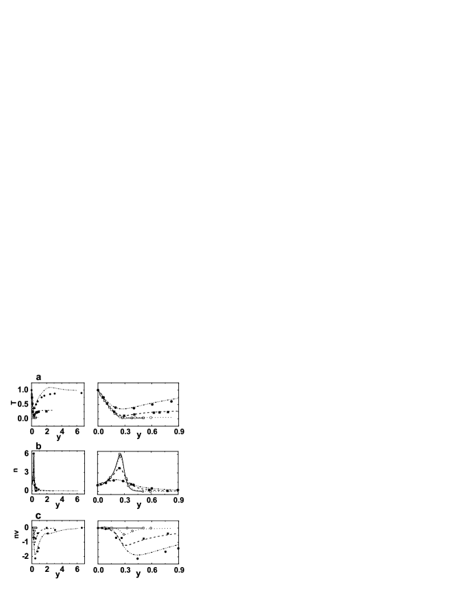
Figure 3: The temperature (a), number density (b) and mass flux $nv$ (c) versus the Eulerian coordinate $y$ at late times, as computed from the low-Mach-number model (symbols) and full hydrodynamics (lines). The scaled parameters are $\Lambda=\sqrt{10}$ and $\varepsilon=\sqrt{5}\cdot 10^{-2}$. The figures on the left and on the right show the same profiles on different scales of height. The scaled times are $t=0.1$ (solid circle, dash-dot-dot line), $0.3$ (solid square, dashed line), $0.5$ (empty circle, dotted line) and $0.85$ (empty square, solid line). The steady state solutions $T_{s}(y)$ and $n_{s}(y)$ are indistinguishable from the respective solid lines.

numerically. Figures 2 and 3 show the steady state temperature and density profiles in the Lagrangian and Eulerian coordinates for $\Lambda=\sqrt{10}$.

Equation (24) enables one to find the critical (minimum) value of $\Lambda$ for the density inversion. At small $\Lambda$ the density decreases monotonically with $m$ (and therefore with $y$). The density inversion is born, at $m=0$, at $\Lambda=\Lambda_{c}$. Therefore, to find $\Lambda_{c}$, we demand that the derivative $n_{s}^{\prime}(m)$ vanish at $m=0$. Using Eq. (24), we can reduce this condition to the equation $I_{0}(\Lambda)=2\Lambda\,I_{1}(\Lambda)$, first obtained in Ref. [18]. Its solution yields $\Lambda_{c}\simeq 1.06569\dots$. At $\Lambda>\Lambda_{c}$ the density reaches its maximum in the Lagrangian point $m_{\ast}=1-\Lambda_{c}/\Lambda>0$. Therefore, the position of the density peak in the Lagrangian coordinate grows with $\Lambda$ monotonically. The respective (scaled) density maximum value is

$$n_{max}=\frac{\Lambda_{c}\,I_{0}^{2}(\Lambda)}{\Lambda\,I_{0}^{2}(\Lambda_{c})}\,.$$ (26)

Using Eq. (25), we can compute the scaled Eulerian coordinate $y_{\ast}$ at which the maximum density maximum occurs:

$$y_{\ast}=\frac{1}{I_{0}^{2}(\Lambda)}\int_{\Lambda_{c}}^{\Lambda}\frac{I_{0}^{2}(\xi)}{\xi}\,d\xi\,.$$ (27)

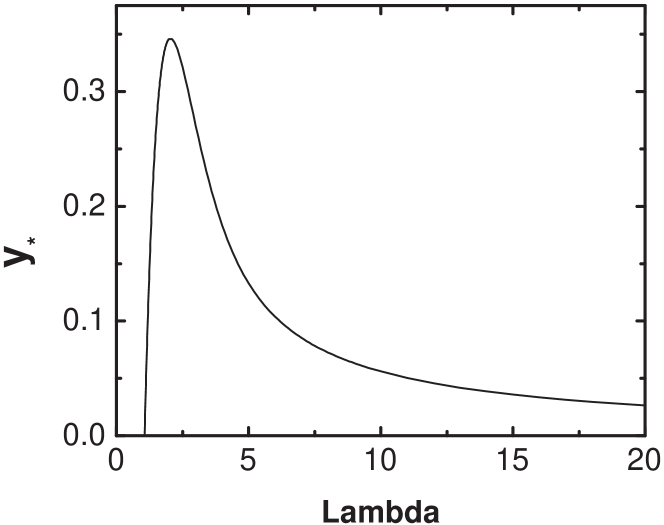
Figure 1: The density peak height in the (scaled) Eulerian coordinate versus $\Lambda$.

The dependence of $y_{\ast}$ on $\Lambda$ is non-monotonic, see Fig. 1. Very close to the density inversion birth (at $\Lambda>\Lambda_{c}$) this dependence is linear: $y_{\ast}\simeq\Lambda/\Lambda_{c}-1$, while at $\Lambda\gg\Lambda_{c}$ one obtains $y_{\ast}\simeq(2\Lambda)^{-1}$. Actually, the integral in Eq. (27) can be calculated analytically, in terms of a hypergeometric function.

4 Formation of a density inversion: Low-Mach-Number flow

Now let us return to the time-dependent problem. Can we exploit the presence of a small parameter $\varepsilon^{2}$ in Eqs. (17) and (18) to simplify the equations? One can expect that the respective terms cannot be neglected during the rapid initial stage of the dynamics. The duration of this stage is of the order of the acoustic time or, in our scaled units, of the order of $\varepsilon$. A comparison of different terms in the momentum equation (17) shows that the typical scaling of the velocity during this stage is $\varepsilon^{-1}\gg 1$. In the physical units, the flow velocity here is comparable to, or larger than, the speed of sound. Correspondingly, at early times the $\varepsilon^{2}$-terms are comparable to, or larger than, the other terms and therefore should be kept.

The situation changes at later times, determined by the inelastic heat losses and heat conduction. Here the characteristic Mach number of the flow becomes small, and we can neglect, in the leading order, the $\varepsilon^{2}$-terms in Eqs. (17) and (18). As the result, the momentum equation (17) is reduced to the hydrostatic condition (20), while in the energy equation (18) one can drop the viscous heating term. The continuity equation (16) remains the same as before. The boundary conditions at $m=0$ do not change, but those at $m=1$ are reduced to $n\,\partial T/\partial m=0$. The boundary condition $n\,\partial v/\partial m=0$ should be dropped altogether.

What is the physical meaning of the reduced model? A low-Mach-number flow proceeds on a time scale that is much longer than the time needed for establishing the (approximate) hydrostatic equilibrium, so the flow does not violate the hydrostatics. Similar reductions of nonlinear time-dependent gas-dynamic problems, that employ a separation of time/length scales, have been successfully used in the context of the dynamics of an optically thin plasma that is cooled by radiation [19]. The presence of a heat loss term in the energy equation makes the latter problem similar to problems of granular dynamics.

The hydrostatic condition immediately yields $p(m,t)\equiv n(m,t)T(m,t)=1-m$, like in the steady state solution! Using it together with the continuity equation (16), we can rewrite the energy equation as an evolution equation for $\omega(m,t)=T^{1/2}(m,t)$:

$$\omega\frac{\partial\omega}{\partial t}=(1-m)\frac{\partial^{2}\omega}{\partial m^{2}}-\frac{\partial\omega}{\partial m}-\Lambda^{2}(1-m)\,\omega\,.$$ (28)

This nonlinear parabolic equation should be solved with two boundary conditions: $\omega(0,t)=1$ and $(1-m)\,\partial\omega/\partial m\to 0$ as $m\to 1$. Notice that the only relevant scaled parameter in the low-Mach-number problem is $\Lambda$.

Once Eq. (28) is solved, we can find $n(m,t)$ and $v(m,t)$:

$$v(m,t)=\frac{\partial}{\partial t}\int_{0}^{m}\frac{dm^{\prime}}{n(m^{\prime},t)}\,.$$ (29)

To transform back to the Eulerian coordinates we use Eq. (19).

Equation (28) was solved numerically with a MATLAB PDE solver. Figure 2 shows an example of numerical solution, at different times, for $\Lambda=\sqrt{10}$. The initial condition for the temperature, $T(m,t=0)=1$, corresponds to a barometric density profile, which looks especially simple in the Lagrangian coordinate: $n(m,t=0)=1-m$. The solution shows cooling of the granular gas because of the inelastic heat losses (see Fig.  2 a). Simultaneously, a density peak develops at an intermediate height (Fig.  2 b). The material flux (Fig.  2 c) is everywhere negative: the material slowly falls from above until the steady-state with a zero mean velocity is reached. An important feature of the time-dependent solution is a transient temperature minimum that develops at intermediate times. It is caused by the fact that the inelastic heat losses are very small at large heights, where the gas density is small. Therefore, the gas cools down relatively fast at intermediate heights, which causes a temperature minimum there. Then a downward heat flux develops that removes the heat from above, finally creating a monotonically decreasing steady state temperature profile. One can see from Fig. 2 that the steady state temperature and density profiles coincide with the analytic solutions. The respective solutions in the Eulerian coordinates are shown in Fig. 3.

5 Formation of a density inversion: Early times

The low-Mach-number theory is invalid at early times, when the hydrostatics has not settled down yet, and the mean flow velocity can reach, or even exceed, the local speed of sound. To investigate these early times, and to check the validity of the low-Mach-number theory at later times, we solved numerically the full set of hydrodynamic equations (16)-(18) in the Lagrangian form. The parameter $\varepsilon$ was taken to be $\sqrt{5}\cdot 10^{-2}\simeq 0.02236$. Equations (16) and (17) were solved with an explicit numerical scheme, based on the standard finite-difference method described in Ref. [20]. The viscous term in Eq. (17) was integrated explicitly, using a two-steps method, which is both stable and accurate. The energy equation (18) was treated implicitly, with a conservative scheme.

We started with simple initial conditions: the constant temperature $T(m,t=0)=1$, the barometric density profile $n(m,t=0)=1-m$ and a zero mean velocity. As expected, the late-time results show good agreement with the predictions of the low-Mach-number theory. Figure 2 shows that, at latest times, the full-hydrodynamics solutions coincide with those obtained with the low-Mach-number theory. At an intermediate time one can see a local increase of the temperature at high altitudes, which is predicted by the full hydrodynamics, but missed by the low-Mach-number theory. The reason for this transient temperature maximum is the relatively large viscous heating that occurs at high altitudes because of a steep velocity gradient there.

The early-time results of the full numerical solution, transformed back to the Eulerian coordinate, are shown in Fig. 4. One can see that the development of the density peak, and the formation of the transient temperature minimum, start already at early times. A more detailed analysis does show differences between the fast and slow theories. Indeed, a necessary condition for the validity of the low-Mach-number theory is the hydrostatic balance condition. This condition looks especially simple in the Lagrangian coordinate: $p(m,t)=1-m$. That is, when the hydrostatics sets in, the plots of the pressure versus $m$, at different times, should collapse into a single straight line. Figure 5 shows the pressure plots at different times. One can see that, at late times, the hydrostatic condition sets in as expected. At early times pressure oscillations are observed, and hydrostatics does not hold. Figure 6 shows the pressure history at the bottom plate $m=0$, or $y=0$. One can see that the pressure undergoes oscillations on the fast time scale of the system $\mathcal{O}(\varepsilon)$. The oscillations rapidly decay with time and, starting from $t\simeq 0.4$, the pressure stays almost constant which implies a low-Mach-number flow.

6 Discussion

We have employed granular hydrodynamics to describe a time-dependent granular flow that gives rise to a density inversion in a vibrofluidized granular system. We have predicted the formation of a transient temperature minimum at intermediate times. The temperature minimum ultimately disappears as the system approaches the steady state with a density inversion. We have also predicted pressure oscillations at early times, when the hydrostatic condition is not yet satisfied.

We hope that the predicted phenomena will be observed in molecular dynamics (MD) simulations and in experiments with vibrofluidized granular beds. The MD simulations should start from the barometric density profile, corresponding to the temperature of the bottom plate. A natural way to initiate the initial state is to first run the simulation with elastic particle collisions. After the barometric profile sets in, the collision rule should be switched into inelastic regime.

The hydrodynamic theory considered in this work is expected to be quantitatively accurate for nearly elastic collisions, $1-r^{2}\ll 1$, and in the dilute limit. The latter condition demands that the maximum number density of the particles be less than, say, $0.2\,n_{c}$, where $n_{c}=2/(\sqrt{3}d^{2})$ is the hexagonal close packing density. The maximum density peak is achieved at the steady state. Therefore, using Eq. (26) and going back to the “physical” density, we can write the dilute regime criterion as

$$\frac{\Lambda_{c}}{I_{0}^{2}(\Lambda_{c})}\,\frac{\sqrt{3}Nd^{2}}{2\lambda L_{x}}\,\frac{I_{0}^{2}(\Lambda)}{\Lambda}<0.2\,.$$ (30)

An alternative form of the same criterion is

$$\frac{I_{0}^{2}(\Lambda)}{\varepsilon\,\Lambda}\,\frac{d}{\lambda}<0.65\,.$$ (31)

We expect that the theory is still valid qualitatively when this criterion is not satisfied, but the maximum density is still less than about $0.5\,n_{c}$. To achieve a better accuracy for such moderately dense flows, one can use the constitutive relations of Jenkins and Richman [11] that account for excluded volume effects.

Acknowledgements

This work was supported by a grant No. 180/02 from the Israel Science Foundation, administered by the Israel Academy of Sciences and Humanities.

Figure 2: The temperature (a), number density (b) and mass flux $nv$ (c) versus the Lagrangian mass coordinate $m$ at late times, as computed from the low-Mach-number model (symbols) and full hydrodynamics (lines). The scaled parameters are $\Lambda=\sqrt{10}$ and $\varepsilon=\sqrt{5}\cdot 10^{-2}$. The scaled times are $t=0.1$ (solid circle, dash-dot-dot line), $0.3$ (solid square, dashed line), $0.5$ (empty circle, dotted line) and $0.85$ (empty square, solid line). The analytic steady state solutions $T_{s}(m)$ and $n_{s}(m)$ are indistinguishable from the respective solid lines.

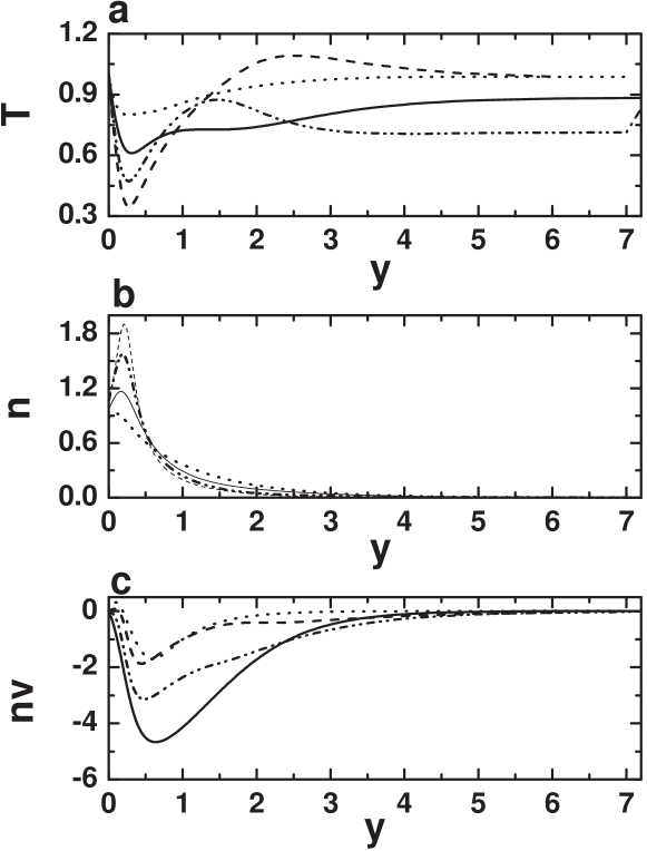
Figure 4: The temperature (a), number density (b) and mass flux $nv$ (c) versus the Eulerian coordinate $y$ at early times, as computed from the full hydrodynamics. The scaled parameters are $\Lambda=\sqrt{10}$ and $\varepsilon=\sqrt{5}\cdot 10^{-2}$. The scaled times are $t=0.01$ (the dotted line), $0.04$ (the solid line), $0.07$ (the dash-dot-dot line) and $0.1$ (the dashed line).

Figure 5: The pressure $p=n\,T$ versus the Lagrangian mass coordinate $m$ at different times, as computed from the full hydrodynamics. The scaled parameters are $\Lambda=\sqrt{10}$ and $\varepsilon=\sqrt{5}\cdot 10^{-2}$. The scaled times are $t=0.01$ (the dashed line), $0.04$ (the dash-dot-dot line), $0.5$ (the solid line) and $0.85$ (the empty circles).

Figure 6: The pressure $p=n\,T$ at the bottom plate $y=0$, versus time, as computed from the full hydrodynamics. The scaled parameters are $\Lambda=\sqrt{10}$ and $\varepsilon=\sqrt{5}\cdot 10^{-2}$.

References

- [1] L. P. Kadanoff. Built upon sand. Rev. Mod. Phys., 71:435, 1999.
- [2] M. A. Hopkins and M. Y. Louge. Inelastic microstructure in rapid granular flows of smooth disks. Phys. Fluids A, 3:47, 1991.
- [3] I. Goldhirsch and G. Zanetti. Clustering instability in dissipative gases. Phys. Rev. Lett., 70:1619, 1993.
- [4] S. McNamara and W. R. Young. Dynamics of a freely evolving, two-dimensional granular medium. Phys. Rev. E, 53:5089, 1996.
- [5] J. S. Olafsen and J. S. Urbach. Clustering, order, and collapse in a driven granular monolayer. Phys. Rev. Lett., 81:4369, 1998.
- [6] T. C. P van Noije and Ernst. M. Kinetic theory of granular gases. In Pöschel and Luding [21], page 3.
- [7] I. Goldhirsch. Granular gases: Probing the boundaries of hydrodynamics. In Pöschel and Luding [21], page 79.
- [8] It has been found recently that fluctuations are anomalously large [22, 23], and their strength decreases very slowly with [22], in the parameter region corresponding to phase separation in driven granular gases. As the result, hydrodynamics can still be invalid in a system of as many as particles [22].
- [9] E. Livne, B. Meerson, and P. V. Sasorov. Symmetry-breaking instability and strongly peaked periodic clustering states in a driven granular gas. Phys. Rev. E, 65:021302, 2002.
- [10] The phase separation instability has been recently observed in molecular dynamics simulations [22, 24, 25], and the subject is rapidly developing [26, 27].
- [11] J. T. Jenkins and M. W. Richman. Kinetic theory for plane flows of a dense gas of identical, rough inelastic circular disks. Phys. Fluids, 28:3485, 1985.
- [12] R. Ramìrez, D. Risso, and P. Cordero. Thermal convection in fluidized granular systems. Phys. Rev. Lett., 85:1230, 2000.
- [13] X. He, B. Meerson, and G. Doolen. Hydrodynamics of thermal granular convection. Phys. Rev. E, 65:030301(R), 2002.
- [14] E. Khain and B. Meerson. Onset of thermal convection in a horizontal layer of granular gas. Phys. Rev. E, 67:021306, 2003.
- [15] L. D. Landau and E. M. Lifshitz. Course of Theoretical Physics, volume 6 Fluid Mechanics. Pergamon, Oxford, 1987.
- [16] It was observed, in some experiments [28, 29] and simulations [18, 29, 30] with vibrofluidized granular materials that, at large heights, the temperature starts increasing with the height. As the particle density at these heights is very small, hydrodynamics might be inapplicable. In any case, most of the density profile is apparently insensitive to the presence of such a temperature inversion, if any.
- [17] Y. B. Zeldovich and Y. P. Raizer. The Physics of Shock Waves and High Temperature Hydrodynamic Phenomena. Academic, New York, 1967.
- [18] J. J. Brey, M. J. Ruiz-Montero, and F. Moreno. Hydrodynamics of an open vibrated granular system. Phys. Rev. E, 63:061305, 2001.
- [19] B. Meerson. Nonlinear dynamics of radiative condensations in optically thin plasmas. Rev. Mod. Phys., 68:215, 1996.
- [20] R. D. Richtmyer and K. W. Morton. Difference Methods for Initial Value Problems. Interscience, New York, 1967.
- [21] T. Pöschel and S. Luding, editors. Granular Gases. Lecture Notes in Physics. Springer, Berlin, 2001.
- [22] B. Meerson, T. Pöschel, P. V. Sasorov, and T. Schwager. Breakdown of granular hydrodynamics at a phase separation threshold. cond-mat/020826.
- [23] A. Barrat and E. Trizac. A molecular dynamics “Maxwell demon” experiment for granular mixtures. Molecular Physics (to appear), 2003. cond-mat/0212054.
- [24] J. J. Brey, M. J. Ruiz-Montero, F. Moreno, and R. García-Rojo. Transversal inhomogeneities in dilute vibrofluidized granular fluids. Phys. Rev. E, 65:061302, 2002.
- [25] M. Argentina, M. G. Clerc, and R. Soto. Van der Waals-like transition in fluidized granular matter. Phys. Rev. Lett., 89:044301, 2002.
- [26] E. Khain and B. Meerson. Symmetry-breaking instability in a prototypical driven granular gas. Phys. Rev. E, 66:021306, 2002.
- [27] E. Livne, B. Meerson, and P. V. Sasorov. Symmetry breaking and coarsening of clusters in a prototypical driven granular gas. Phys. Rev. E, 66:050301(R), 2002.
- [28] E. Clement and J. Rajchenbach. Fluidization of a bidimensional powder. Europhys. Lett., 16:133, 1991.
- [29] K. Helal, T. Biben, and J. P. Hansen. Local fluctuations in a fluidized granular media. Physica A, 240:361, 1997.
- [30] R. Ramìrez and R. Soto. Temperature inversion in granular fluids under gravity. cond-mat/0210471.