Kelvin modes of a fast rotating Bose-Einstein Condensate

Abstract

Using the concept of diffused vorticity and the formalism of rotational hydrodynamics we calculate the eigenmodes of a harmonically trapped Bose-Einstein condensate containing an array of quantized vortices. We predict the occurrence of a new branch of anomalous excitations, analogous to the Kelvin modes of the single vortex dynamics. Special attention is devoted to the excitation of the anomalous scissors mode.

.1 Introduction

The existence of the macroscopic wave function describing a quantum fluid imposes a velocity flow curl free everywhere except on singularity lines known as vortices. Around these lines, the circulation of the velocity is non zero and is quantized in unit of $h/m$ where $m$ is the mass of the particles of the fluid. Recent experiments have demonstrated the nucleation of such quantized vortices in stirred gaseous Bose-Einstein condensates (BEC) Matthews00 ; Madison00 ; AboShaer01 ; Hodby01 .

Multiple quantized vortices are energetically unstable in harmonic traps so that for large rotation frequencies, Bose-Einstein condensates nucleate several singly quantized vortices that were observed to form regular triangular lattices known as Abrikosov lattices AboShaer01 ; Madison00b ; Haljan01 . In this configuration, the circulation of the velocity field over a circle orthogonal to the rotation axis and of radius $R$ much larger than the vortex interspacing, is simply $\pi R^{2}n_{v}h/m$, where $n_{v}$ is the density of the vortex lines. This is the same formula as that of the velocity field of a rigid body rotating at the angular velocity

$$\Omega_{0}=n_{v}\frac{h}{2m}.$$ (1)

The dynamical properties of a single vortex line were first studied by Lord Kelvin Thomson80 and his results were transposed to quantum fluids Pitaevskii61 ; Isoshima99 ; Svidzinsky00 . For an excitation of wave vector $k$ propagating along the rotation axis, the dispersion relation $\omega_{\rm K}$ of these modes (Kelvin modes or kelvons) is:

$$\omega_{\rm K}\sim\frac{\hbar k^{2}}{2m}\ln\left(1/k\xi\right),$$ (2)

where $\xi=(8\pi\rho a)^{-1/2}$ is the healing length giving the vortex core diameter, $a$ the scattering length characterizing atom binary interactions and $\rho$ is the density of the gas. These modes present the very peculiar feature that they only exist with a single helicity as recently proved in the experiments of Bretin02 . Indeed, the Kelvin-Helmholtz theorem that constrains the vorticity to move along with the fluid imposes an angular momentum equal to $-\hbar$ to the Kelvin modes.

Although the problem of studying the dynamics of a vortex array seems more involved at first sight, it is considerably simplified for long wavelength perturbations. Indeed, in this case a coarse grain averaging method permits to smooth the discrete nature of vortices. In the case of a homogeneous condensate, it was shown that excitations of wavevector $k$ propagating transversally to the rotation axis satisfy the Tkatchenko dispersion relation Tkachenko69 ; Baym83 :

$$\omega^{2}_{\rm T}=\frac{\hbar\Omega_{0}}{4m}k^{2},$$

where $\Omega_{0}$ is the effective angular frequency of the condensate defined by (1). The Tkatchenko modes are elastic excitations of the lattice and have been recently investigated theoretically also in the presence of harmonic traps Anglin02 . First experimental evidences for such modes has been reported in jila03 .

In this paper we use the coarse grain method to study the eigenmodes of a rotating Bose-Einstein condensate confined by a harmonic trap using a fully hydrodynamic approach including vorticity Sedrakian01 . In addition to the usual collective modes exhibited by the condensate in the absence of rotation, we identify an additional branch, analogous to the Kelvin modes exhibited by a single vortex line. With respect to the Tkatchenko modes, whose frequencies vanish in the Thomas Fermi limit Anglin02 , the Kelvin excitations emerging from our hydrodynamic picture approach a finite value in the Thomas-Fermi limit. In the case of elongated traps their frequencies actually scale like $\omega^{2}_{z}/\omega_{\perp}$, for a fixed value of $\Omega_{0}/\omega_{\perp}$.

The paper is organized as follows: in Sect. B we develop the formalism of rotational hydrodynamics in the presence of harmonic trapping and derive the general equations (10) for the dispersion law of the linearized excitations. In Sect. C we briefely summarize the results for the surface excitations which represent a natural generalization of the modes exhibited by non rotating Bose-Enstein condensates. Section D is devoted to the scissors mode where an anomalous mode of Kelvin nature is predicted. The properties of the scissors oscillations for a rotating condensate are discussed in detail using the formalism of linear response theory. Finally in Sect. E we obtain a general dispersion relation for the Kelvin modes in elongated traps.

.2 Rotational hydrodynamics and elementary excitations

It is well known that in the so-called Thomas-Fermi regime, where the mean field interaction dominates over the quantum pressure, the dynamics of a non rotating condensate can be described by the classical equations of hydrodynamics:

$$\partial_{t}\rho = -\mathbf{\nabla}\left(\rho\mathbf{v}\right)$$ (3)

$$m\partial_{t}\mathbf{v} = -\mathbf{\nabla}\left(U_{t}+g\rho+mv^{2}/2\right),$$ (4)

where $\rho$ is the local particle density, $g=4\pi\hbar^{2}a/m$ is the coupling constant characterizing the interatomic force and $\mathbf{v}$ the velocity field satisfying the irrotational condition $\mathbf{\nabla}\times\mathbf{v}=0$. In the case of cylindrical harmonic trapping,

$$U_{t}=\frac{m}{2}\left(\omega_{\perp}^{2}(x^{2}+y^{2})+\omega_{z}^{2}z^{2}\right)\;,$$

the hydrodynamic equations (3) and (4) admit a class of analytic solutions sandro96 whose frequencies have been confirmed experimentally with high accuracy.

In the presence of vortex lines the hydrodynamical formalism must be modified. Here we will employ a simplified procedure, by assuming that the characteristic wavelength of excitations is large enough so that we can average all the physical quantities over domains containing several vortices. In this case the average lab frame velocity field $\mathbf{\bar{v}}$ is no longer curl-free. Since each vortex carries a flux $h/m$, the average vorticity of the flow is:

$$\mathbf{\bar{\Omega}}=\frac{\mathbf{\nabla\times\bar{v}}}{2}=n_{v}\frac{h}{2m}\mathbf{u},$$ (5)

where $n_{v}$ is the vortex surface density and the unit vector $\mathbf{u}$ is the local direction of the vortex lines. According to equation (5), the average vorticity $\mathbf{\bar{\Omega}}$ characterizes the local vortex distribution: its direction indicates the orientation of the vortex lines while its modulus is proportional to the vortex density.

Like in Sedrakian01 ; Cozzini02 , we shall simply assume that the average velocity field and density satisfy classical hydrodynamical equations, including rotational terms, namely:

$$\left\{\begin{array}[]{rcl}\partial_{t}\bar{\rho}&=&-\mathbf{\nabla}\left(\bar{\rho}\mathbf{\bar{v}}\right)\\ m\partial_{t}\mathbf{\bar{v}}&=&-\mathbf{\nabla}\left(U_{t}+g\bar{\rho}+m\frac{\bar{v}^{2}}{2}\right)-m\left(\mathbf{\nabla\times\bar{v}}\right)\times\mathbf{\bar{v}},\end{array}\right.$$ (6)

A stationary solutions of equations (6) is given by:

$$\left\{\begin{array}[]{rcl}\mathbf{\bar{v}_{0}}&=&\mathbf{\Omega_{0}\times r}\\ g\bar{\rho}_{0}/m&=&\mu-\left(\omega_{\perp}^{2}-\Omega_{0}^{2}\right)(x^{2}+y^{2})/2-\omega_{z}^{2}z^{2}/2,\end{array}\right.$$ (7)

where $\mu$ is the chemical potential and $\mathbf{\Omega_{0}}=\Omega_{0}{\bf u}_{z}$ characterizes the vortex density and direction according to equation (5). As expected, the stationary velocity field is equivalent to that of a rigid body rotating at angular velocity $\mathbf{\Omega}_{0}$, while the density is described by the usual Thomas-Fermi profile with the trapping potential $U_{t}$ corrected by the centrifugal potential $U_{c}=-m\Omega_{0}^{2}(x^{2}+y^{2})/2$. The static behavior described above has been verified experimentally. In particular, the modification of the transverse trapping is used to measure experimentally the effective angular velocity $\mathbf{\Omega_{0}}$ AboShaer01 ; Haljan01 . More interesting effects concern the study of the dynamics of the condensate. In Cozzini02 the hydrodynamic equations have been used to study the time evolution of a condensate containing a vortex array, following the sudden switch on of a static deformation in the plane of rotation. This produces peculiar non linear effects that have been experimentally observed in Haljan01 . In the following we will focus on the behaviour of the linearized solutions which can be derived by looking for small perturbations of the the density and velocity field:

$$\left\{\begin{array}[]{rcl}\bar{\rho}&=&\bar{\rho}_{0}+\delta\rho\\ \mathbf{\bar{v}}&=&\mathbf{\Omega_{0}\times r}+\delta\mathbf{v},\end{array}\right.$$

with respect to the equilibrium values (in this case, $\delta{\bf v}$ can be interpreted as the velocity in the rotating frame). If the characteristic wavelength of the perturbation is much larger than the vortex spacing, the “averaged” hydrodynamical equations (6) can still be applied and, in the frame rotating at the angular velocity $\mathbf{\Omega_{0}}$, they read, in linear approximation,

$$\partial_{t}\delta\rho = \mathbf{\nabla^{\prime}}\left(\bar{\rho}_{0}\delta\mathbf{v}\right)$$ (8)

$$\partial_{t}\delta\mathbf{v} = -\mathbf{\nabla^{\prime}}\left(\frac{g\delta\rho}{m}\right)-2\mathbf{\Omega}_{0}\times\delta\mathbf{v},$$ (9)

where $\mathbf{\nabla}^{\prime}$ denotes the derivation with respect to the coordinates in the rotating frame. The system of equations (8,9) constitutes the starting point of our analysis. We will study its eigenmodes and show that the spectrum, in addition to the usual “phonon” modes displays a new class of solutions carrying negative angular momentum and that can be physically regarded as Kelvin excitations.

Let us set $\partial_{t}=-i\omega^{\prime}$ in equations (8,9). Using equation (9), we can then express $\delta\mathbf{\bar{v}}$ as a function of $\delta\rho$ as

$$\delta\mathbf{v}=\frac{1}{\omega^{\prime 2}-4\Omega_{0}^{2}}\left[i\omega^{\prime}\left({\bf f}\right)_{\perp}+2\mathbf{\Omega}_{0}\times{\bf f}\right]-\frac{1}{i\omega^{\prime}}\left({\bf f}\right)_{\|},$$

where ${\bf f}=-\mathbf{\nabla}^{\prime}\left(g\delta\rho\right)/m$ and $\left({\bf f}\right)_{\|}$ and $\left({\bf f}\right)_{\perp}$ are, respectively, the projections of ${\bf f}$ on the directions parallel and orthogonal to $z$.

Inserting this expression for the velocity field in the linearized mass conservation equation (8) , we get a closed equation for the density fluctuations that can be written as

$$i\omega^{\prime}\left(\omega^{\prime}{}^{2}-4\Omega_{0}^{2}\right)\delta\rho={\cal A}\cdot\delta\rho,$$ (10)

where ${\cal A}$ denotes the linear operator

$${\cal A}\cdot\delta\rho = -\nabla^{\prime}_{\perp}\left[\frac{g\rho_{0}}{m}\left(i\omega^{\prime}\nabla^{\prime}_{\perp}\delta\rho+2\mathbf{\Omega_{0}}\times\nabla^{\prime}_{\perp}\delta\rho\right)\right]$$

$$+\nabla^{\prime}_{\|}\left[\frac{g\rho_{0}}{m}\left(\frac{\omega^{\prime}{}^{2}-4\Omega_{0}^{2}}{i\omega^{\prime}}\nabla^{\prime}_{\|}\delta\rho\right)\right],$$

and $\rho_{0}$ is the equilibrium density profile (7). Equations (10) and (.2) are the main result of this paper. Simple solutions can be found in the form of polynomials.

Let us stress again that the calculation of $\omega^{\prime}$ is performed in the rotating frame. The corresponding frequency $\omega$ in the lab frame is obtained through the simple relation $\omega^{\prime}=\omega-m_{z}\Omega_{0}$, where $\hbar m_{z}$ is the angular momentum of the excitation along the rotation axis. Since both $\delta\rho$ and its complex conjugate are solutions of (.2) we find that for any solution with angular momentum $m_{z}$ and eigenfrequency $\omega^{\prime}$, there should be an other solution with angular momentum $-m_{z}$ and frequency $-\omega^{\prime}$. Since the unperturbed state (condensate rotating at angular velocity $\mathbf{\Omega_{0}}$) is the ground state of the system in the rotating frame, the physical solutions carrying energy $\hbar\omega^{\prime}$ should correspond to positive frequencies $\omega^{\prime}$.

Note also that the equation (10) is valid for $\omega^{\prime}\not=0$ and $\omega^{\prime 2}\not=4\Omega_{0}^{2}$ and that these two special cases must be treated separately. The case $\omega^{\prime 2}-4\Omega_{0}^{2}=0$ does not lead to any new mode. The case $\omega^{\prime}=0$ is instead more interesting since it is related to the Tkatchenko’s modes, as stressed in the introduction. Starting the analysis back from equations (8) and (9), we can show that the density perturbation $\delta\rho$ of a zero energy modes depends only on the radial coordinate $r_{\perp}=\sqrt{x^{2}+y^{2}}$ and that the velocity field is given by:

$$\left\{\begin{array}[]{rcl}v_{z}&=&0\\ {\bf v}_{\perp}&=&\displaystyle{\frac{g}{2m\Omega_{0}^{2}}}\,\mathbf{\Omega}_{0}\times\mathbf{\nabla}\delta\rho.\end{array}\right.$$

In the case where $\delta\rho$ is parabolic, this zero energy mode can be simply interpreted as a modification of $\Omega_{0}$, i.e. a change of the vortex density.

The rest of the paper is devoted to the solution of equation (.2) for special cases of physical interest. We will first discuss the surface oscillations then the scissors modes, that will be shown to exhibit a kelvon-like branch. Finally we will derive the general dispersion law for the Kelvon modes working in the geometry of elongated traps.

.3 Surface modes

Surface modes are characterized by the form $\delta\rho=(x\pm iy)^{l}$ and carry angular momentum $m_{z}=\pm l$. Inserting this Ansatz in the differential equation (10) yields the following equation for the eigenfrequencies $\omega^{\prime}_{\pm l}$ in the rotating frame:

$$\omega^{\prime}_{\pm l}{}^{2}\pm 2\Omega_{0}\omega^{\prime}_{\pm l}-l\left(\omega_{\perp}^{2}-\Omega_{0}^{2}\right)=0.$$

The positive solution of this equation reads:

$$\omega^{\prime}_{\pm l}=\sqrt{l\omega_{\perp}^{2}-(l-1)\Omega_{0}^{2}}\mp\Omega_{0},$$

or, in the laboratory frame,

$$\omega_{\pm l}=\sqrt{l\omega_{\perp}^{2}-(l-1)\Omega_{0}^{2}}\pm(l-1)\Omega_{0}.$$

Contrarily to what happens in the case of a non-rotating condensate, the two modes are no longer degenerate, and the degeneracy lift amounts to:

$$\Delta\omega_{l}=\omega_{+l}-\omega_{-l}=2(l-1)\Omega_{0}.$$ (11)

This result is valid for any $l$ LargeL but can be checked for some special cases previously reported in the literature.

In the $l=1$ case (dipole motion) one finds $\Delta\omega=0$. In this case the eigenfrequencies are actually unaffected by the rotation since $\omega_{\pm l}=\omega_{\perp}$ irrespectively of the value of $\Omega_{0}$. This is not surprising since we know that the generalized Kohn theorem Dobson94 implies that the center of mass motion is determined only by the frequency of the harmonic trap.

The case $l=2$ is also well documented, both theoretically and experimentally Zambelli01 ; Chevy00 . Using sum-rule approach, it can be shown in particular that the degeneracy lift amounts to:

$$\Delta\omega=2\frac{\langle\ell_{z}\rangle}{m\langle r_{\perp}^{2}\rangle},$$ (12)

$\ell_{z}$ is the angular momentum per particle along $z$ of the unperturbed condensate. Since the unperturbed velocity field is rigid-like, the angular momentum is given by the classical formula $\langle\ell_{z}\rangle=m\langle r_{\perp}^{2}\rangle\Omega_{0}$. Inserting this relation in (12) yields result (11) for $l=2$.

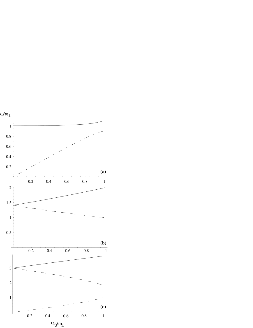
Figure 1: Absolute values of the lab frame frequencies of the $m_{z}=+1$ (full line), $m_{z}=-1$ (dashed line) and anomalous (dash-dotted line) scissors modes for three trap geometries. (a): cigar shaped, with $\omega_{\perp}=10\omega_{z}$. (b): isotropic trap with $\omega_{z}=\omega_{\perp}$. In this case the frequency of the anomalous mode is zero. (c): pancake trap with $\omega_{z}=\sqrt{8}\omega_{\perp}$.

.4 Scissors modes

The scissors modes are associated with a density fluctuation $\delta\rho=(x\pm iy)z$ carrying angular momentum $m_{z}=\pm 1$ along the $z$ axis. Using equation (.2), one finds that the eigenfrequencies $\omega^{\prime}$ must satisfy the non trivial cubic equation:

$$\omega^{\prime}{}^{3}\pm 2\Omega_{0}\omega^{\prime 2}-\omega^{\prime}\left(\omega_{z}^{2}+\omega^{2}_{\perp}-\Omega_{0}^{2}\right)\mp 2\Omega_{0}\omega_{z}^{2}=0.$$ (13)

This equation is analogous to that found by the authors of Sedrakian01 using the tensor virial method. Two of the resulting modes can be identified with the usual $m_{z}=\pm 1$ scissors previously studied in the case of non-rotating Bose-Einstein condensates dgo . The splitting between these two modes is easily calculated when $\Omega_{0}\to 0$. In the laboratory frame one finds $\Delta\omega=2\Omega_{0}\omega_{z}^{2}/(\omega_{z}^{2}+\omega_{\perp}^{2})$ in agreement with the sum rule result of Zambelli01 that was confirmed experimentally in Hodby02 . This splitting is at the origin of the gyroscopic effect investigated in Stringari01 in the presence of a single vortex line. The third mode predicted by (13) has instead no analog for $\Omega_{0}=0$. A sign analysis shows that the frequency $\omega^{\prime}_{a}$ of this anomalous mode is positive for $m_{z}=-1$. Just like the kelvons, this new scissor mode can only exist with negative helicity. The analog of this mode in the case of a single vortex line was investigated by Svidzinsky00 . The solutions of equation (13) as a function of $\Omega_{0}$ are shown in Fig.1 for different trapping geometries. The interpretation of this mode is straightforward for an isotropic trap: in this case, the anomalous mode is associated with an overall rotation of the condensate and of its lattice. In an isotropic trap this rotation indeed costs no energy and the frequency in the lab frame is exactly zero.

For very deformed traps, i.e. for $|\omega_{\perp}^{2}-\omega_{z}^{2}|\gg\Omega_{0}^{2}$, the anomalous mode is associated to a scissors mode of the vortex lattice while the density profile remains almost at rest.

In the second part of this section we discuss how the scissors modes, and in particular the anomalous mode, can be excited and observed by suddenly tilting the trapping potential in the ($x,z$) plane. To this purpose we make use of the formalism of linear response theory. Let us apply a perturbing potential of the form

$$\delta U=\epsilon z^{\prime}(x^{\prime}+iy^{\prime})e^{-i\omega^{\prime}t}+\epsilon^{*}z^{\prime}(x^{\prime}-iy^{\prime})e^{i\omega^{\prime}t}$$

in the rotating frame. Using the hydrodynamical equations, we find that the density and the vorticity will be perturbed as

$$\delta\rho = \epsilon\lambda_{\omega^{\prime}}z^{\prime}(x^{\prime}+iy^{\prime})e^{-i\omega^{\prime}t}+\epsilon^{*}\lambda_{\omega^{\prime}}^{*}z^{\prime}(x^{\prime}-iy^{\prime})e^{i\omega^{\prime}t},$$

$$\delta\mathbf{\Omega} = \epsilon\mu_{\omega^{\prime}}e^{-i\omega^{\prime}t}{\bf u}_{+}+\epsilon^{*}\mu_{\omega^{\prime}}^{*}e^{i\omega^{\prime}t}{\bf u}_{-},$$

where ${\bf u}_{\pm}={\bf u}_{x}\pm i{\bf u}_{y}$. The quantities $\lambda$ and $\mu$ can be calculated using the hydrodynamical equations and one finds the result

$$\lambda_{\omega^{\prime}} = \frac{2\Omega_{0}\omega_{z}^{2}+\omega^{\prime}(\omega_{\perp}^{2}+\omega_{z}^{2}-\Omega_{0}^{2})}{gP(\omega^{\prime})}$$ (14)

$$\mu_{\omega^{\prime}} = -\frac{\omega^{\prime}\Omega_{0}}{mP(\omega^{\prime})},$$ (15)

where $P(\omega^{\prime})={\omega^{\prime}}^{3}+2\Omega_{0}{\omega^{\prime}}^{2}-\omega^{\prime}(\omega_{z}^{2}+\omega_{\perp}^{2}-\Omega_{0}^{2})-2\Omega_{0}\omega_{z}^{2}$ is a polynomial whose roots fix the eigenfrequencies of the system (see Eq.(13)). Notice that the change $\delta{\bf\Omega}_{0}$ in the vorticity, lying in the ($x,y$) plane, actually corresponds to a rotation of the vector lattice. This rotation could be imaged experimentally, allowing, together with the changes in the shape of the atomic cloud, for a direct identification of the various scissors modes.

On the one hand, the expectation value $\langle z^{\prime}(x^{\prime}-iy^{\prime})\rangle\equiv\int{\rm d}^{3}r\delta\rho z^{\prime}(x^{\prime}-iy^{\prime})$ can be written as

$$\langle z^{\prime}(x^{\prime}-iy^{\prime})\rangle=\epsilon\chi_{\omega}^{\rm HD}e^{-i\omega^{\prime}t}+\epsilon^{*}\left(\chi_{\omega}^{\rm HD}\right)^{*}e^{-i\omega^{\prime}t},$$

and one obtains the result

$$\chi_{\omega^{\prime}}^{\rm HD}=\lambda_{\omega^{\prime}}\frac{\pi R_{z}^{3}R_{\perp}^{4}}{6}.$$ (16)

for the hydrodynamic response function $\chi_{\omega}^{\rm HD}$.

On the other hand, this expectation value can be calculated using the formalism of quantum mechanics. Using first order perturbation theory the linear response function relative to the operator $F=\sum_{k=1}^{N}z^{\prime}_{k}(x^{\prime}_{k}-iy^{\prime}_{k})$ can be in fact written as

$$\chi_{\omega^{\prime}}^{\rm QM}=\sum_{n}\frac{|\langle n|F^{\dagger}|0\rangle|^{2}}{\hbar\omega^{\prime}-E^{\prime}_{n}}-\frac{|\langle n|F|0\rangle|^{2}}{\hbar\omega^{\prime}+E^{\prime}_{n}},$$ (17)

where $|0\rangle$ and $|n\rangle$ are respectively the ground state and the excited states of the many body system and $E^{\prime}_{n}$ are the associated eigenenergies in the rotating frame. From (17), we see that the poles of $\chi_{\omega}$ are the eigenfrequencies of the system. Moreover, the sign of the residue at the pole gives its helicity: positive residues are associated with positive helicity (i.e. with modes excited by $z(x+iy)$ ), and negative residues are instead associated with negative helicity.

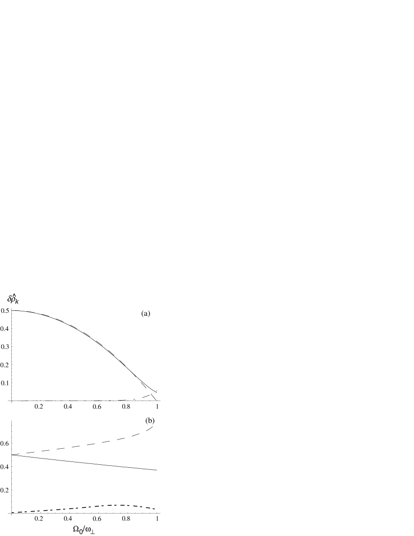
Figure 2: Density coupling of the scissor $m_{z}=+1$ (full line), $m_{z}=-1$ (dashed line) and anomalous (dash dotted line) transitions for different trapping geometries. (a) Elongated trap ($\omega_{\perp}=10\omega_{z}$) and (b) pancake trap ($\omega_{z}=\sqrt{8}\omega_{\perp}$). )

By identifying $\chi^{\rm QM}$ and $\chi^{\rm HD}$ and by close examination of eqs. (14), we can conclude that :

1. The anomalous mode has positive energy in the rotating frame and its angular momentum is $m=-1$.

2. For $\omega_{z}<\omega_{\perp}$, we have $\omega_{\rm a}<0$ . For cigar geometries the anomalous mode is then associated to a thermodynamical instability of the vortex lattice in the laboratory frame Reverse .

3. On the contrary, for $\omega_{z}>\omega_{\perp}$, we have $\omega_{\rm a}>0$. For pancake geometries, the vortex lattice is stable versus scissor perturbations.

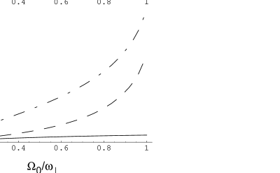
Figure 3: Change of vorticity of the scissor $m_{z}=+1$ (full line), $m_{z}=-1$ (dashed line) and anomalous (dash dotted line) transitions for different trapping geometries. (a) Elongated trap ($\omega_{\perp}=10\omega_{z}$) and (b) pancake trap ($\omega_{z}=\sqrt{8}\omega_{\perp}$). For these modes the change of vorticity is associated with a change of direction of the vortical lattice. )

Let us now consider the special case of the sudden tilting at $t=0$ of the longitudinal axis of the trap in the lab frame. This excitation leads to the following perturbing potential:

$$\delta U=\alpha xzY(t)=\alpha z(x+iy)+\alpha z(x-iy)Y(t),$$

where $Y$ is the Heavyside step-function equal to $0$ for $t<0$ and 1 otherwise. Expressed in the rotating frame, $\delta U$ reads:

$$\delta U=\left(\alpha z(x+iy)e^{i\Omega_{0}t}+\alpha z(x-iy)e^{-i\Omega_{0}t}\right)Y(t).$$

The Fourier transform of this perturbation then yields:

$$\epsilon_{\omega^{\prime}}=\alpha(\pi\delta(\omega^{\prime}+\Omega_{0})+i/(\omega^{\prime}+\Omega_{0})).$$

According to equation (14) and (15), the induced density and vorticity changes are given by:

$$\delta\rho = \left(\int{\rm d}\omega^{\prime}\epsilon_{\omega^{\prime}}\lambda_{\omega^{\prime}}e^{-i\omega^{\prime}t}\right)z(x+iy)+{\rm c.c.}$$ (18)

$$\delta\mathbf{\Omega} = \left(\int{\rm d}\omega^{\prime}\epsilon_{\omega^{\prime}}\mu_{\omega^{\prime}}e^{-i\omega^{\prime}t}\right){\bf u}_{+}+{\rm c.c.}.$$ (19)

These integrals can be calculated using standard integration techniques in the complex plane. In particular, $\delta\rho$ and $\delta\mathbf{\Omega}$ present terms oscillating at the driving frequency $\-\Omega_{0}$, as well as at the scissor frequencies $\omega_{\pm 1}$ and $\omega_{\rm a}$. Let us introduce the Fourier components of these modes:

$$\delta\rho = \left(\delta\hat{\rho}_{0}e^{i\Omega_{0}t}+\sum_{k=\pm 1,a}\delta\hat{\rho}_{k}e^{-i\omega^{\prime}_{k}t}\right)z(x+iy)+{\rm c.c.}$$

$$\delta\mathbf{\Omega} = \left(\delta\hat{\Omega}_{0}e^{i\Omega_{0}t}+\sum_{k=\pm 1,a}\delta\hat{\Omega}_{k}e^{-i\omega^{\prime}_{k}t}\right){\bf u}_{+}+{\rm c.c.}.$$

According to equations (18) and (19), $\delta\hat{\rho}_{k}$ and $\delta\hat{\Omega}_{k}$ are given, respectively, by the residues of $\lambda_{\omega^{\prime}}/(\omega^{\prime}+\Omega_{0})$ and $\mu_{\omega^{\prime}}/(\omega^{\prime}+\Omega_{0})$ . We have plotted the density response $\delta\hat{\rho}_{k}$ on Fig. (2). We see that the anomalous mode weight is very weak, both in the pancake and cigar traps (except for $\Omega_{0}\sim\omega_{\perp}$). The behavior of the vorticity is dramatically different, as observed on Fig. (3). Indeed, while the anomalous mode remains weak in the case of an elongated trap (Fig. (3.a)), we see that it dominates the dynamics in the pancake geometry. This effect should be detectable experimentally by imaging the orientation of the vortex lattice.

.5 Kelvin spectrum

The study of the scissor modes has revealed the existence of an anomalous kelvon-like mode with angular momentum $m_{z}=-1$. For very elongated traps ($\omega_{\perp}\gg\omega_{z}$), the corresponding solution is given by:

$$\omega^{\prime}\sim 2\Omega_{0}\frac{\omega_{z}^{2}}{\omega_{\perp}^{2}-\Omega_{0}^{2}}$$

showing that the frequency of the anomalous mode goes to zero in the limit of small $\omega_{z}$. In what follows, we shall generalize this result by looking for more general solutions of (11) satisfying $\omega^{\prime}\sim\omega_{z}^{2}$ when $\omega_{z}\rightarrow 0$. In this approximation, we can restrict equation (.2) to non vanishing terms in $\omega$ and $\omega_{z}$, which yields the simplified equation

$$\nabla^{\prime}_{\perp}\left[2\rho_{0}\mathbf{\Omega_{0}}\times\nabla^{\prime}_{\perp}\delta\rho\right]+\nabla^{\prime}_{\|}\left[\rho_{0}\left(\frac{4\Omega_{0}^{2}}{i\omega^{\prime}}\nabla^{\prime}_{\|}\delta\rho\right)\right]=0.$$ (20)

Let us now write the density perturbation as the most general polynomial of order $p+l$ associated to angular momentum $m_{z}=-l$:

$$\delta\rho=r_{\perp}^{l}e^{-il\theta}\sum_{q=0}^{q_{m}}b_{q}z^{2q}r_{\perp}^{p-2q}+...,$$

where the expression is restricted to terms of leading order in the $(r_{\perp},\theta,z)$ cylindrical coordinates and where $q_{m}$ is the highest $q$ such that $p-2q\geq 0$. According to equation (20), the coefficients $b_{q>0}$ must satisfy the recursive relation:

$$b_{q}=-\frac{(p-2q+2)(p+1-2q)\Omega_{0}^{2}}{\left(-l\Omega_{0}\omega_{\perp}^{2}\omega^{\prime}+(p-2q)(p-2q+1)\Omega_{0}^{2}\omega_{z}^{2}\right)}b_{q-1},$$

while, for $q=0$,

$$\left(-l\Omega_{0}\omega_{\perp}^{2}+p(p+1)\frac{\Omega_{0}^{2}}{\omega^{\prime}}\omega_{z}^{2}\right)b_{0}=0.$$ (21)

In order to get non vanishing $b_{q}$, the coefficient of $b_{0}$ in equation (21) must cancel out. This ensures the quantization of the eigenfrequencies, since we must have:

$$\omega^{\prime}=p(p+1)\frac{\Omega_{0}\omega_{z}^{2}}{l\left(\omega_{\perp}^{2}-\Omega_{0}^{2}\right)}.$$ (22)

This dispersion relation represents the generalization of the classical Kelvin law to the case of a rotating gas confined in a harmonic trap. Like kelvons, these new modes have always a negative angular momentum and possess a quadratic behavior for large $p$. If $R_{z}$ and $R_{\perp}$ denote the condensate radii in the longitudinal and transverse directions respectively, these two quantities are related by (see (7))

$$\omega_{z}^{2}R_{z}^{2}=\left(\omega_{\perp}^{2}-\Omega^{2}\right)R_{\perp}^{2}.$$

Moreover, $\delta\rho$ is a polynomial of order $p$ in $z$. The quantity $k=p/R_{z}$ can then be interpreted as the longitudinal wave vector of the excitation. Using the relation $\Omega_{0}=n_{v}h/2m$ equation (22) yields, for large quantum numbers $p$,

$$\omega^{\prime}=N_{v}\frac{\hbar}{lm}k^{2},$$

where $N_{v}=n_{v}\pi R_{\perp}^{2}$ is the number of vortices present in the condensate. This dispersion law is very similar to equation (2), except for the logarithmic factor that vanished through the averaging procedure.

Note also that equation (22) is singular for $l=0$. This is due to the fact that in this case $\omega^{\prime}\sim\omega_{z}$ so terms neglected in (20) must be taken into account. In this case, there is no decoupling between the phonon and kelvon branches, and no simple analytical expression can be extracted.

- (1) Also at Laboratoire de la Matière Condensée, Collège de France, Paris, France.
- (2) Unité de Recherche de l’Ecole normale supérieure et de l’Université Pierre et Marie Curie, associée au CNRS.
- (3) M. R. Matthews, B. P. Anderson, P. C. Haljan, D. S. Hall, C. E. Wieman, and E. A. Cornell, Phys. Rev. Lett. 83, 2498 (2000).
- (4) K. W. Madison, F. Chevy, W. Wohlleben and J. Dalibard, Phys. Rev. Lett. 84, 806 (2000).
- (5) E. Hodby, G. Hechenblaikner, S. A. Hopkins, O.M. Maragò and C. J. Foot, Phys. Rev. Lett. 88, 010405 (2001).
- (6) J.R. Abo-Shaer, C. Raman, J. M. Vogels and W. Ketterle, Science 292, 476 (2001).
- (7) K. W. Madison, F. Chevy, W. Wohlleben and J. Dalibard, Rev. Mod. Opt. 47, 2715 (2000).
- (8) P.C. Haljan, I. Coddington, P. Engels and E.A. Cornell, Phys. Rev. Lett. 87, 210403 (2001).
- (9) W. Thomson (Lord Kelvin), Phil. Mag. 10 155 (1880).
- (10) L.P. Pitaevskii, Sov. Phys. JETP, 13 451, (1961).
- (11) T. Isoshima and K. Machida, Phys. Rev. A. 59, 2203 (1999).
- (12) A.A. Svidzinsky and A.L. Fetter, Phys. Rev. A 62, 063617 (2000).
- (13) V. Bretin, P. Rosenbusch, F. Chevy, G.V. Shlyapnikov and J. Dalibard, Phys. Rev. Lett. 90, 100403 (2003) .
- (14) V.K. Tkachenko, Sov. Phys. JETP 29, 945 (1969).
- (15) G. Baym and E. Chandler, J. Low. Temp. Phys, 50, 57 (1983); G. Baym, cond-mat/0305294.
- (16) J. R. Anglin and M. Crescimanno, cond-mat/0210063.
- (17) I. Coddington, P. Engels, V. Schweikhard and E. A. Cornell, cond-mat/0305008
- (18) A. Sedrakian and I. Wasserman, Phys. Rev. A 63, 063605 (2001).
- (19) S. Stringari, Phys. Rev. Lett. 77, 2360 (1996)
- (20) M. Cozzini and S. Stringari, Phys. Rev. A 67 041602 (2003).
- (21) J.F. Dobson Phys. Rev. Lett. 73, 2244 (1994).
- (22) must be compatible with the large wavelentgh hypothesis, that is should be much larger than the vortex interspacing.
- (23) F. Zambelli et S. Stringari, Phys. Rev. Lett. 81, 1754 (1998).
- (24) F. Chevy, K. Madison and J. Dalibard, Phys. Rev. Lett. 85, 2223 (2000).
- (25) D. Guery-Odelin and S. Stringari, Phys. Rev. Lett. 83, 4452 (1999).
- (26) S. Stringari, Phys. Rev. Lett. 86, 4725 (2001).
- (27) E. Hodby, S.A. Hopkins, G. Hechenblaikner, N.L. Smith and C.J. Foot, cond-mat/0209634.
- (28) It also means that, from an experimental point of view, the anomalous mode will correspond to a scissor excitation rotating in the positive direction.