Noise dressing of the correlation matrix of factor models

Abstract

We study the spectral density of factor models of multivariate time series. By making use of the Random Matrix Theory we analytically quantify the effect of noise dressing on the spectral density due to the finiteness of the sample. We consider a broad range of models ranging from one factor models in time and frequency domain to hierarchical multifactor models.

The extraction of information from a multivariate time series is a central issue in many applications. Several methods has been introduced to this end, ranging from principal component analysis to clustering methods mardia ; cluster . The simplest and more widespread models of multivariate time series are factor models. In these models the dynamics of each variable is the linear combination of a given number of factors plus an idiosyncratic noise term. The coefficients of the linear combination and the intensity of the noise terms are specific of each variable and assumed for simplicity to be time independent. Examples of such models are Capital Asset Pricing Model or CAPM (one factor) and Arbitrage Pricing Theory (multifactor) in the financial domain campbell . Another class of factor models describes the dynamics of the variables driven by one or more sinusoidal signals of given frequency with each variable characterized by a different phase. This kind of models as been recently applied to gene expression analysis during cell cycle obtained by microarray data maritan ; brown . In this second case the variables are following the common factor(s) in frequency domain rather than in real time. The more general multifactor model for $N$ variables $x_{i}(t)$ ($i=1,...,N$) can be written as

$$x_{i}(t)=\sum_{j=1}^{K}\gamma_{i}^{(j)}f_{j}(t)+\gamma_{i}^{(0)}\epsilon_{i}(t).$$ (1)

In this equation $K$ is the number of factors $f_{j}(t)$, $\gamma_{i}^{(j)}$ is a constant describing the weight of factor $j$ in explaining the dynamics of the variable $x_{i}$, and $\epsilon_{i}(t)$ is a Gaussian zero mean noise term with unit variance. In Eq.(1) we assume that the factors are uncorrelated one with each other, i.e. $\langle f_{i}(t)f_{j}(t)\rangle=\delta_{ij}$, where the symbol $\langle...\rangle$ indicates an average in time. Also the noise terms are uncorrelated one with each other and with the factors, i.e. $\langle\epsilon_{i}(t)\epsilon_{j}(t)\rangle=\delta_{ij}$ and $\langle f_{i}(t)\epsilon_{j}(t)\rangle=0$. Since in the rest of this paper we are interested in studying the linear correlation coefficients, without loss of generality we assume that all the variables $x_{i}$ have zero mean and unit variance. These assumptions fix the value $(\gamma_{i}^{(0)})^{2}=1-\sum_{j}(\gamma_{i}^{(j)})^{2}$.

Multivariate methods are designed to extract the information on the number of factors and on the composition of the groups. On the other hand any real experiment is performed on a finite sample of $T$ records for each variable and the measured quantities in the analysis are unavoidably dressed by noise. In this letter we study the role of the noise in dressing the properties of the spectral density of the correlation matrix. The correlation matrix C is the $N\times N$ symmetric matrix whose entries are the linear correlation coefficient between each pair of variable $x_{i}$ and $x_{j}$. The object of our study is the spectral density of the sample correlation matrix ${\bf\hat{C}}$. The square root of the eigenvalues of ${\bf\hat{C}}$ are called singular values. We will make use of the Random Matrix Theory metha to compute the role of noise dressing on the spectrum of correlation matrices of factor models. Most of the results we derive are valid in the limit of $N\to\infty$ and $T\to\infty$, even though for real large matrices the approximation is quite good. The application of Random Matrix Theory to the noise dressing of correlation matrices has been recently addressed denby ; sengupta ; sosh and applied to the study of financial correlation matrices bouchaud ; stanley ; sornette . In Ref. bouchaud ; stanley the null hypothesis used to compare real sample correlation matrices is a model of uncorrelated variables, or in our language a zero factor model or random model. In the random model each variable is described only by a random Gaussian variable $\epsilon_{i}(t)$. The corresponding class of random matrices is called Wishart matrix in statistical literature. The correlation matrix is the identity matrix and the spectral density is $\rho(\lambda)=N\delta(\lambda-1)$. The noise dressing of the spectrum of the sample correlation matrix has been derived in denby ; sengupta . In the limit $T,N\to\infty$, with a fixed ratio $Q=T/N\geq 1$, the spectral density of the correlation matrix is given by

$$\rho(\lambda)=\frac{T}{2\pi\lambda}\sqrt{(\lambda_{max}-\lambda)(\lambda-\lambda_{min})},$$ (2)

where $\lambda_{min}^{max}=(1+1/Q\pm 2\sqrt{1/Q})$. Since the procedure used to obtain this result is very similar to the one we use below, here we summarize it briefly. One introduces the resolvent

$${\cal G}(z)=\sum_{n=1}^{N}\frac{1}{z-\lambda_{n}},$$ (3)

which is related to the spectral density through

$$\rho(\lambda)=\frac{1}{\pi}\lim_{\epsilon\to 0}Im[{\cal G}(\lambda-i\epsilon)].$$ (4)

The resolvent is equal to ${\cal G}(z)=\partial_{z}\ln\det(z-\rho)$. By making use of the replica trick and by performing a saddle point approximation one finds an equation for the ensemble average of the resolvent $G(z)=\langle{\cal G}(z)\rangle_{ens}$ and through Eq. (4) the spectral density is obtained. The symbol $\langle...\rangle_{ens}$ indicates an average on the ensemble of variables.

Even if the random model can be sometimes a starting null hypothesis, a factor model should be used as null hypothesis when one suspects the presence of common factors in the dynamics of an ensemble of variables. As a first example we shall consider the one factor model in which the dynamics of each variable is controlled by a single common factor. The equations describing the one factor model is given by Eq. (1) with $K=1$. The parameter $\gamma_{i}^{2}$ gives the fraction of variance explained by the common factor $f(t)$. It is direct to show that the correlation coefficient between variable $i$ and $j$ is $\gamma_{i}\gamma_{j}$. The correlation matrix of the one factor model can therefore be written as ${\bf C}={\bf A}+{\bf bb^{+}}$, where ${\bf A}=diag(1-\gamma_{i}^{2})$ is a diagonal $N\times N$ matrix and ${\bf b^{+}}=(\gamma_{1},...,\gamma_{N})$ is a row vector. The characteristic equation of ${\bf C}$ can be calculated by using the Sherman-Morrison formula numrec , and the result is

$$\det({\bf C}-{\bf I_{N}}\lambda)=\prod_{i=1}^{N}(1-\gamma_{i}^{2}-\lambda)\left[1+\sum_{i=1}^{N}\frac{\gamma_{i}^{2}}{1-\gamma_{i}^{2}-\lambda}\right]=0.$$ (5)

In the case of a degenerate one factor model, i.e. when $\gamma_{i}=\gamma$ for all values of $i$, the characteristic equation can be solved and the spectrum is composed by a large eigenvalue $\lambda_{1}=1+(N-1)\gamma^{2}\simeq N\gamma^{2}$ and $N-1$ degenerates eigenvalues $\lambda_{i}=1-\gamma^{2}$ where $i=2,...,N$ sornette . We are not able to solve Eq.(5) in the non degenerate case, but we are able to provide an approximate form of the spectrum when $N$ is large. In the non-degenerate case we can still expect a spectral density composed by a large eigenvalue (high part) and $N-1$ small eigenvalues (low part). The large eigenvalue can be obtained by putting to zero the term in square brackets in Eq.(5). The largest eigenvalue is much larger than $1-\gamma_{i}^{2}$ for any $i$ and we can therefore approximate the characteristic equation as $\sum\gamma_{i}^{2}/\lambda_{1}\simeq 1$, i.e. $\lambda_{1}\simeq\sum_{i=1}^{N}\gamma_{i}^{2}=N\langle\gamma_{i}^{2}\rangle_{ens}$. In order to have an insight on the spectral density for the other $N-1$ eigenvalues we assume that the $\gamma_{i}$ are distributed according to a given probability density $P(\gamma_{i})$. We make the ansatz that the distribution of $\lambda_{i}$ is given by $P(\lambda)=P(\gamma_{i})d\gamma_{i}/d\lambda$ where $\gamma_{i}=\sqrt{1-\lambda}$. The idea behind this ansatz is that the relation between eigenvalues and $\gamma_{i}$ is the same as in the degenerate case. For example if $\gamma_{i}$ is distributed uniformly in a subinterval $[m-d,m+d]$ of $[0,1]$, the distribution of the $N-1$ eigenvalues is given by $P(\lambda)=(4d)^{-1}(1-\lambda)^{-1/2}$. Note that under our ansatz this part of the spectrum is bounded from above by the value $\lambda=1$. In panel (a) of Fig. 1 we show the low part of the spectral density of a one factor model describing $N=2000$ variables. The $\gamma_{i}$ are distributed exponentially with $\bar{\gamma}=0.25$. The line is the theoretical prediction based on our ansatz. The agreement between data and the ansatz is quite good.

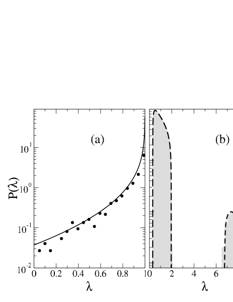
Figure 1: (a) The low part of the spectrum of a single realization of a non degenerate one factor model (circle). In this case $N=2000$ and $\bar{\gamma}=0.25$. The continuous line is the prediction based on the ansatz discussed in the text. (b) Spectral density of a degenerate one factor model. The gray areas are the average over $1000$ numerical simulations of a one factor model of $N=100$ variables for $T=500$ time steps. The value of $\gamma$ is $0.25$. The dashed line is the theoretical prediction.

We now consider the noise dressing of the spectrum due to the finiteness of the sample. In other words we assume that our data are described by a one factor model (degenerate or not) and we assume that we have $T$ synchronous records for each $x_{i}$ variable. By using the arguments of Ref. sengupta we can prove that the ensemble averaged resolvent of a one factor model of $N$ variables for $T$ time steps is determined by the equation

$$G(z)=\frac{T}{z-\sum_{i=1}^{N}\frac{\lambda_{i}}{T-\lambda_{i}G(z)}}.$$ (6)

For the degenerate one factor model discussed above the equation for the resolvent is a third degree algebraic equation supplement , which can be solved exactly. The spectral density can be obtained analytically from Eq.s (4) and (6), even if the expression is quite long. As expected the spectral density is different from zero in two intervals, one for the $N-1$ small eigenvalues and one for the large eigenvalue $\lambda_{1}$. Numerical calculations and analytical considerations show that the low part of the spectrum is well fitted by a functional form of Eq.(2). Moreover the width of the two intervals scale with the parameter of the model as $\Delta_{0}\sim(1-\gamma^{2})\sqrt{N/T}$ and $\Delta_{1}\sim N\gamma^{2}/\sqrt{T}$, where $\Delta_{0}$ ($\Delta_{1}$) is the width of the low (high) part of the spectrum. Panel (b) of Fig. 1 shows the comparison of theoretical prediction and numerical simulations of a degenerate one factor model. The agreement is very good in the whole range of eigenvalues. It is worth noting that such an agreement is obtained also when $T<N$.

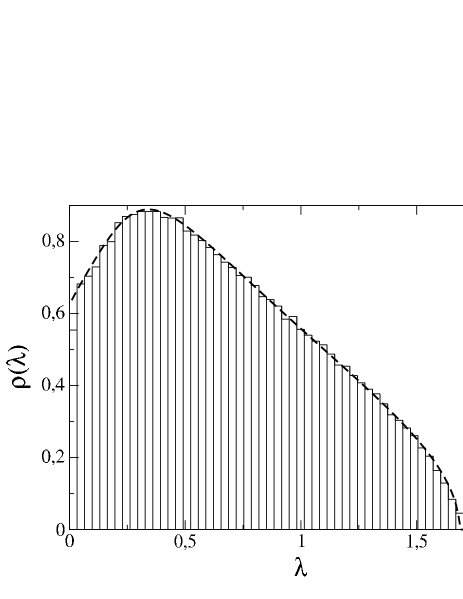
Figure 2: Low part of the spectral density of a completely non degenerate one factor model, i.e. a one factor model in which $\gamma_{i}$ is distributed uniformly between 0 and 1. The dashed line is the theoretical result obtained through the theory developed in the text.

We come now to the more complicated case of non degenerate one factor model. In order to find the spectrum one should solve Eq.(5) for all the eigenvalues and then solve the $(N+1)$th degree polynomial of Eq.(6). This task is too complicated even numerically. We use a different approach making use of the fact that $N$ is large. The sum in the denominator of Eq. (6) is split in a term for $\lambda_{1}$ plus a sum over the remaining $N-1$ small eigenvalues. This last term can be computed as $N-1$ times the average of $\lambda/(T-\lambda G(z))$ over $P(\lambda)$ introduced in our ansatz. In other words, Eq. (6) for the resolvent becomes

$$G(z)=\frac{T}{z-\frac{\lambda_{1}}{T-\lambda_{1}G(z)}-(N-1)\langle\frac{\lambda_{i}}{T-\lambda_{i}G(z)}\rangle_{ens}},$$ (7)

where $\lambda_{1}\simeq 1+(N-1)\langle\gamma_{i}^{2}\rangle_{ens}$. In general the average term in (7) is not a rational function and therefore Eq.(7) cannot be reduced to an algebraic equation in $G$. In order to solve the complex transcendental equation (7) we introduce a simple algorithm. The average term in (7) depends typically on the dispersion of the $P(\gamma_{i})$ at the second order. Therefore the low part of the spectrum of a non degenerate one factor model with a small dispersion in $\gamma_{i}$ is not very different from a degenerate one-factor model with $\gamma_{eff}=\sqrt{\langle\gamma_{i}^{2}\rangle_{ens}}$. We can therefore use the value of the resolvent of this effective degenerate one factor model as the starting point for the searching of the solution of Eq. (7). Quite surprisingly this method works also when the dispersion of the $\gamma_{i}$ is high. For example for a uniform distribution of $\gamma_{i}$, the average term in Eq. (7) involves two inverse hyperbolic tangent functions supplement . In Fig. 2 we show the low part of the spectrum for a completely degenerate one factor model, i.e. a model in which $\gamma_{i}$ is uniformly distributed between $0$ and $1$. We see that the agreement between the theory and the simulations is very good. A similar good agreement is observed for exponentially distributed $\gamma_{i}$ supplement . It is worth noting that in the general case of a degenerate one factor model the low part of the spectrum is not compatible with a Wishart form of Eq.(2).

The results obtained for the one factor model can be easily extended to multifactor model. When the factors are stochastic and uncorrelated one with each other the structure of the correlation matrix is given by the composition of the groups of variables correspondent to the factors. The simplest case is when each variable belongs to one and only one groups, i.e. its dynamics is determined by only one factor and by the idiosyncratic noise. In this case the correlation matrix is block diagonal. The correlation coefficient between variables belonging to different groups is zero, while, when the variables $i$ and $j$ belong to the same group $k$, the correlation coefficient is $\gamma_{i}^{(k)}\gamma_{j}^{(k)}$. The spectral density of this kind of models is simply given by the superposition of the spectral densities of $K$ one factor models. The theory of noise dressing follows directly from Eq. (6) in which the number of distinct eigenvalues is $2K$. The equation for $G(z)$ is therefore an algebraic equation of degree $2K+1$. Again if the distributions of $\gamma_{i}^{(k)}$ are given, one can solve the non degenerate case by using the same arguments of the one factor model. Clearly the computational task increases with the number of factors.

An interesting generalization of multifactor models occurs when there is a hierarchical overlap between different groups. To give a concrete example, let us consider a portfolio of stocks. As a first approximation we can consider the portfolio as composed by a large group following a common factor (the market factor in CAPM) and a certain number of groups homogeneous in economic activity following a sectoral factor, such as, for example, the oil companies or the technological group. In this case the composition of the groups induces a hierarchical structure to the correlation matrix. Also this kind of models can be solved. We present here a simple example in which the $N$ variables follow a common factor with a constant $\Gamma$. Moreover the set of variables is divided in two groups. We have $n_{1}$ variables following the first subfactor with constant $\gamma_{1}$ and $n_{2}=N-n_{1}$ variables following the second subfactor with constant $\gamma_{2}$. The correlation matrix of this model is a block matrix composed by a block $n_{1}\times n_{1}$ matrix whose entries are $\Gamma^{2}+\gamma_{1}^{2}$ and $1$ on the diagonal and a block $n_{2}\times n_{2}$ matrix whose entries are $\Gamma^{2}+\gamma_{2}^{2}$ and $1$ on the diagonal. The elements in the out diagonal block submatrices are equal to $\Gamma^{2}$.

The spectrum of this matrix is composed by two large eigenvalues given by

$$\lambda_{\pm}=\frac{1}{2}(2+\gamma_{1}^{2}(n_{1}-1)+\gamma_{2}^{2}(n_{2}-1)+\Gamma^{2}(n_{1}+n_{2}-2)$$

$$\pm\sqrt{A^{2}+\Gamma^{4}(n_{1}+n_{2})^{2}+2A\Gamma^{2}(n_{1}-n_{2})}),$$ (8)

where $A=(\gamma_{1}^{2}(n_{1}-1)-\gamma_{2}^{2}(n_{2}-1))$ and $n_{1}-1$ eigenvalues equal to $1-\Gamma^{2}-\gamma_{1}^{2}$ and $n_{2}-1$ eigenvalues equal to $1-\Gamma^{2}-\gamma_{2}^{2}$. Again by making use of Eq. (6) it is possible to find the effect of noise dressing by solving the corresponding 5th degree algebraic equation supplement . To give the general idea behind the derivation of result (8) and of its generalization to more complex hierarchical models, we note that correlation matrix of degenerate hierarchical factor models can be written in terms of the identity matrix and unit matrices ${\bf J}_{mn}$ (i.e. a $m\times n$ matrix consisting of all 1s). These matrices form a closed algebra under multiplication, for example ${\bf J}_{nm}{\bf J}_{mp}=m{\bf J}_{np}$. The determinant leading to the characteristic equation is directly obtained by using the block submatrices in which the correlation matrix can be partitioned. The above mentioned algebraic properties allows to reduce the characteristic equation in terms of $\det(a{\bf I}_{n}+b{\bf J}_{nn})=a^{n-1}(a+bn)$.

The last class of model we consider is given by a one factor model in which the synchronization with the factor is in frequency rather than in time domain. Specifically, let us consider a factor model in which the dynamics of the variables is described by the equation

$$x_{i}(t)=\gamma\sqrt{2}\sin(\omega t+\phi_{i})+\gamma^{(0)}\epsilon_{i}(t).$$ (9)

The ensemble average of the product of two variables in two distinct instants of time can be written as $\langle x_{i}(t)x_{j}(t^{\prime})\rangle_{ens}=C_{ij}D_{tt^{\prime}}$, where $C_{ij}=\delta_{ij}$ and $D_{tt^{\prime}}=(\gamma^{2}\cos(\omega(t-t^{\prime}))+(1-\gamma^{2})\delta_{tt^{\prime}})$. The model described in Eq. (9) is the first approximation of the dynamics of the level of expression of genes during cell cycle as detected in microarray experiments maritan ; brown . In this case the frequency $\omega$ is related to the duration of the cell cycle. Microarray experiments have usually a very small number of time points compared with the number of variables (genes). This fact leads to an heavy dressing of the correlation matrix by noise, and hence a careful characterization of the noise dressing is even more important in this case. In order to find the effect of noise dressing by using Random Matrix Theory we need to find the spectral density of the matrices ${\bf C}=(C_{ij})$ and ${\bf D}=(D_{tt^{\prime}})$ sengupta . In this case ${\bf C}$ is the identity matrix. The spectrum of ${\bf D}$ can be found and it consists of two large eigenvalues

$$d_{1,2}=\frac{\gamma^{2}}{2}\left(T\pm\frac{\sin\omega T}{\sin\omega}\right)+(1-\gamma^{2}),$$ (10)

and $T-2$ eigenvalues equal to $d_{i}=(1-\gamma^{2})$, where $i=3,...,T$. The equation for the resolvent is in this case (cfr. Eq.s (21-23) of Ref. sengupta )

$$G(z)=\sum_{i=1}^{T}\frac{1}{z-Q(z)d_{i}},$$ (11)

where $Q(z)$ is the solution of the equations

$$Q(z)=\frac{N}{T}\frac{1}{1-R(z)},~{}~{}~{}~{}~{}R(z)=\frac{1}{T}\sum_{i=1}^{T}\frac{d_{i}}{z-d_{i}Q(z)}.$$ (12)

The equation for $G(z)$ is a 4th degree algebraic equation that can be solved exactly supplement .

In conclusion we have shown that the application of Random Matrix Theory allows to solve analytically the problem of the noise dressing of the spectral density of the correlation matrix of a large class of factor models. This class includes one factor model in time and frequency domain and hierarchical and non hierarchical multifactor models. The main idea of the approach we are proposing can be summarized as follows: (i) find the spectrum of the degenerate factor model; this usually accounts to find the few distinct eigenvalues characterizing the spectrum. (ii) Find the effect of the noise dressing in the degenerate case by using Eq. (6); this implies the finding of roots of a low degree polynomial. (iii) Try to solve the non degenerate case by averaging over the distribution of $\gamma$ parameters on the same lines of what has been done here for one factor model (see Eq.(7)). Our results can be applied in many different disciplines including economics, finance, molecular biology and in general in any study in which factor models can constitute a good starting point for modeling the simultaneous dynamics of many variables.

References

- (1) K. V. Mardia, J. T. Kent and J. M. Bibby, Multivariate Analysis, (Academic Press, San Diego, 1979).
- (2) M. R. Anderberg, Cluster Analysis for Applications, (Academic Press, 1973).
- (3) Y. J. Campbell, A. W. Lo, A. C. Mackinlay The Econometrics of Financial Markets, (Princeton University Press, Princeton, 1997).
- (4) N. S. Holter et al., Proc. Nat. Acad. Sci. USA 97, 8409 (2000).
- (5) O. Alter, P. O. Brown and D. Botstein, Proc. Nat. Acad. Sci. USA 97, 10101 (2000).
- (6) M. Metha, Random Matrices (Academic Press, New York, 1995).
- (7) L. Denby and C. L. Mallows, Computing Sciences and Statistics: Proceedings of the 23rd Symposium on the Interface, edited by E.M. Keramidas, (Interface Foundation, Fairfax Station, VA, 1991), pp.54-57.
- (8) A. M. Sengupta and P. P. Mitra, Phys. Rev. E 60, 3389 (1999).
- (9) A. Soshnikov, J. Stat. Phys., 108, 1033 (2002).
- (10) L. Laloux, et al., Phys. Rev. Lett. 83, 1467 (1999).
- (11) V. Plerou, et al., Phys. Rev. Lett. 83, 1471 (1999).
- (12) Y. Malevergne and D. Sornette, preprint available at http://xxx.lanl.gov/cond-mat/0210115.
- (13) The interested reader can ask for supplementary material to lillo@santafe.edu.
- (14) W. H. Press, et al., Numerical Recipes (Cambridge Univ. Press, Cambridge, UK, 1992).