Naive Mean Field Approximation for the Error Correcting Code

Abstract

Solving the error correcting code is an important goal with regard to communication theory. To reveal the error correcting code characteristics, several researchers have applied a statistical-mechanical approach to this problem. In our research, we have treated the error correcting code as a Bayes inference framework. Carrying out the inference in practice, we have applied the NMF (naive mean field) approximation to the MPM (maximizer of the posterior marginals) inference, which is a kind of Bayes inference. In the field of artificial neural networks, this approximation is used to reduce computational cost through the substitution of stochastic binary units with the deterministic continuous value units. However, few reports have quantitatively described the performance of this approximation. Therefore, we have analyzed the approximation performance from a theoretical viewpoint, and have compared our results with the computer simulation.

I Introduction

Within the framework of an error-correcting code, a sender encodes a message with redundant information added to the transmitted sequence, and a receiver obtains the noise-corrupted sequence through a noisy transmitting channel. Decoding process of the error-correcting code is to restore the transmitted message from the received sequence that is corrupted through the transmitting process.

Sourlas suggested that the error-correcting code can be dealt with Bayesian inference, and proposed an encoding model where all possible combinations of $r$-bits must be multiplied as the redundant information just like the Mattis model Mattis76 . Sourlas also showed that the channel capacity of the model can reach the theoretical limit, called the Shannon bound Shannon48 in the limit of $r\rightarrow\infty$. Unfortunately, under the condition $r\rightarrow\infty$, the transmitting speed becomes to $0$, so that the model with large $r$ is not practical. Recently, however, Kabashima & Saad pointed out that the Sourlas encoding model with a small $r$, – for example $r=2,3$ –, is capable of good restoration ability with a practical transmitting speed Kabashima99 .

In this paper, we also treat this problem according to a Bayesian inference framework. This framework is based on estimating the restored message occurrence probability (posterior) from both the prior probability meaning the original message generation probability and the likelihood, which depends on the corruption process model.

One strategy using Bayesian inference is to use a message which maximizes the posterior probability. This method is called maximum a posteriori (posterior) probability (MAP) inference. Given a corrupted sequence, the MAP inference accepts as the restored result the message which maximizes the posterior probability. From the statistical mechanical point of view, the logarithm of the posterior probability can be regarded as the energy, so we can consider the MAP inference as an energy minimization problem.

Another strategy is to use inference in which we consider the expectation value with respect to the maximized marginal posterior probability at each site’s thermal equilibrium as the original message. This method is called maximizer of the posterior marginals (MPM) inferenceRujan93 Sourlas94 Nishimori00 . From the statistical mechanical point of view, the MPM inference corresponds to minimization of the free energy. In the MAP inference, the posterior probability is given for each candidate of sequences. In contrast, in the MPM inference, the posterior marginal probability is given for each bit in the sequence, and the state which has the largest posterior probability is chosen as the restored state for each bit. Hence, to find a optimal bit sequence through the MPM inference, we should compare the posterior probability for each bit, and this requires that we calculate the thermal average for each sequence bit. Recently, the MPM inference has been discussed with regard to error correcting code Rujan93 Sourlas94 Nishimori00 . Ruján pointed out the effectiveness of carrying out a decoding procedure not at the ground state, but at a finite temperatureRujan93 . Sourlas used the Bayes formula to re-derive the finite-temperature decoding of Rujan’s result under more general conditions Sourlas94 . Finite-temperature decoding corresponds to the MPM inference, while decoding at the ground state corresponds to the MAP inference. Comparison of the restoration ability of the MPM inference to that of the MAP inference with regard to the error rate per bit has shown that, the MPM inference is superior to the MAP inference Rujan93 Nishimori00 .

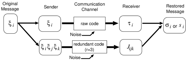
Figure 1: Schematic diagram of a framework for the error correcting code.

To consider the error correcting code from a statistical mechanical perspective, we denoted the message length, where the message is represented by a binary unit sequence, as $N$, and assumed that each unit can take a binary state $\{-1,+1\}$. The number of feasible message combinations in this case would reach $2^{N}$, making it hard to find a correct message among the numerous candidates. Thus, to apply the MAP or MPM inference in a practical way, we usually have to adopt some kind of gradient descent algorithm, such as the Glauber dynamics, despite a risk that the solution will be captured by local minima. Moreover, applying the MPM inference may take more computational time than applying the MAP inference. In the MAP inference, once the system reaches a macroscopic equilibrium state, each pixel value can be properly determined with a probability of $1$. On the other hand, when the system reaches a macroscopic equilibrium state in the MPM inference, each unit value cannot be deterministicly decided because the probabilities for each binary state have finite values in finite-temperature decoding. Therefore, we need to calculate the thermal averages for each unit, and this requires many samplings. In this paper, we discuss an approximation that replaces the stochastic binary units with deterministic analog units which can take $[-1,+1]$ continuously. In other words, we introduce deterministic dynamics into the MPM inference to avoid the need to sample for the thermal average. In statistical mechanics, this approximation is sometimes called the “naive mean field (NMF)” approximation Bray86 . The purpose of the NMF approximation has usually been to enable deterministic analog units to emulate the behavior of stochastic binary units. This approximation has been applied to several combinatorial optimization problems, such as the traveling salesman problem (TSP) Hopfield86 .

One important advantage of applying the NMF approximation is that the calculation cost is reduced since we can avoid calculating the thermal average which requires many samplings in stochastic dynamics. However, the NMF approximation has typically been applied as a mere approximation in algorithm implementation, so few researchers who have used the NMF approximation have investigated its quantitative ability - e.g., the approximation accuracy. In this paper, we discuss the quantitative ability of the NMF approximation in the MPM inferenceShouno02 .

Nishimori & Wong formulated the image restoration problem and the error correcting code from the statistical-mechanical perspective by introducing mean field models for binary image restoration, and analyzed this model theoretically through the replica method. We have applied the NMF approximation to the formulation, and analyzed the model through the replica method in the manner of Bray et al Bray86 .

In the field of neural networks, a network model using the NMF approximation is sometimes called an analog neural network. Roughly speaking, Hopfield & Tank’s network is a result of applying the NMF approximation to the optimization network proposed by Kirkpatrick Kirkpatrick83 Hopfield86 . Therefore, a Hopfield-Tank type network can be regarded as a kind of analog neural network. The formulation of this kind of optimization network is very similar to that of the Sourlas encoding model with $r=2$. In our study, we applied the NMF approximation to the Sourlas encoding model with $r\geq 2$, which is called ‘r-body interaction’ from a statistical-mechanical viewpoint, so that our formulation can be considered a natural extension of a Hopfield-Tank type network with higher-order dimension interactions.

In Sec. II, we formulate the error-correcting code using Bayes inference in the manner of Nishimori & Wong’s formulationNishimori00 .

In Sec. III, we compare the results between from our analysis to those of a computer simulation. Within the limits of the mean field approximation, our results agreed with the simulation results.

II Model and Analysis

II.1 Formulation of the Error Correcting Code

In this section, to make this paper self-contained, we explain the error correcting code in the manner of Nishimori & Wong Nishimori00 . Fig. 1 shows a schematic diagram of the error correcting code. On the sender side, the original signal is represented by $\bm{\xi}$, and each element is a binary unit that takes binary states $\xi_{i}=\{-1,+1\}$ for $i=1\cdots N$. The number of elements means the message length which can be denoted as $N$.

Through the transmission channel, the signals being sent are degraded by noise, so redundant information is needed to enable retrieval of the original message. The error-correcting code has been discussed from a Bayesian inference point of view Rujan93 Sourlas94 Nishimori00 . In the manner of the Sourlas code Sourlas94 , the redundant message is produced from the $r$-units product:

$$\xi_{i_{1}}\xi_{i_{2}}\cdots\xi_{i_{r}},$$ (1)

where the indices satisfy $1\leq i_{1}<i_{2}<\cdots<i_{r}\leq N$. The sender transmits the redundant message $\xi_{i_{1}}\xi_{i_{2}}\cdots\xi_{i_{r}}$ for all possible combinations of the indices. Thus, the redundant message length becomes ${}_{N}C_{r}$. In addition, we assumed that the original message $\{\xi_{i}\}$ has a uniform prior probability:

$$P_{s}(\bm{\xi})=\frac{1}{2^{N}}\quad{\text{for any }}\bm{\xi}.$$ (2)

On the receiver side, degraded signals are observed since transmission channels ares noisy. In this paper, received signals $\bm{\tau}$ correspond to the original message $\bm{\xi}$ (whose elements consists of $\xi_{i}\>(i=1\cdots N)$) and their elements are denoted as $\tau_{i}\>(i=1\cdots N)$, while signals $\bm{J}$ (whose elements consists of $J_{i_{1}\cdots i_{r}}\>(1\leq i_{1}<\cdots<i_{r}\leq N)$) correspond to the redundant message whose elements consists of $\xi_{i_{1}}\cdots\xi_{i_{r}}$. The receiver should be able to estimate the original message $\bm{\xi}$ from the received signals $\bm{\tau}$, $\bm{J}$.

To apply Bayesian inference to estimate the original message, we should consider the posterior probability based on observation:

$$P(\bm{\xi}|\bm{J},\bm{\tau})=\frac{P_{\mathrm{out}}(\bm{J},\bm{\tau}|\bm{\xi})P_{s}(\bm{\xi})}{\mathrm{Tr}_{\left\{\bm{\xi}\right\}}P_{\mathrm{out}}(\bm{J},\bm{\tau}|\bm{\xi})P_{s}(\bm{\xi})}$$ (3)

where $P_{\mathrm{out}}(\bm{J},\bm{\tau}|\bm{\xi})$ is a conditional probability of the observed signal which can be regarded as the probability expression of the corrupting process in the communication channel.

In this study, we assumed the communication channel is a Gaussian channel:

$$P_{\mathrm{out}}(\bm{J},\bm{\tau}|\bm{\xi}) =P(\bm{J}|\bm{\xi})P(\bm{\tau}|\bm{\xi})$$

$$=\prod_{i_{1}<\cdots<i_{r}}P(J_{i_{1}\cdots i_{r}}|\bm{\xi})\prod_{i=1}P(\tau_{i}|\bm{\xi})$$ (4)

$$P(J_{i_{1}\cdots i_{r}}|\bm{\xi}) =\left(\frac{N^{r-1}}{J^{2}\pi r!}\right)^{1/2}$$

$$\times\exp\left(-\frac{N^{r-1}}{J^{2}r!}\left(J_{i_{1}\cdots i_{r}}-\frac{j_{0}r!}{N^{r-1}}\xi_{i_{1}}\cdots\xi_{i_{r}}\right)^{2}\right)$$ (5)

$$P(\tau_{i}|\bm{\xi}) =\frac{1}{\sqrt{2\pi\tau^{2}}}\exp\left(-\frac{1}{2\tau^{2}}\left(\tau_{i}-\tau_{0}\xi_{i}\right)^{2}\right)$$ (6)

The first term in Eq.(4) corresponds to the noise of the redundant message channel, and the second term corresponds to the noise of the original message channel. The random variable $J_{i_{1}\cdots i_{r}}$ is i.i.d. according to a normal distribution whose mean is $\frac{j_{0}r!}{N^{r-1}}\xi_{i_{1}}\cdots\xi_{i_{r}}$. and whose variance is $2J^{2}r!/N^{r-1}$. The random variable $\tau_{i}$ is i.i.d. according to a normal distribution whose mean is $\tau_{0}\xi_{i}$ and whose variance is $\tau^{2}$. Thus, we can describe the transmission channel characteristics using the parameters $j_{0}$, $J$, $\tau_{0}$, and $\tau$.

Substituting Eqs.(2) and (4) into Eq.(3), we can denote the posterior probability as:

$$P(\bm{\xi}|\bm{J},\bm{\tau})=$$

$$\quad\frac{1}{Z}\exp\left(\displaystyle\frac{2j_{0}}{J^{2}}\sum_{i_{1}<\cdots<i_{r}}J_{i_{1}\cdots i_{r}}\xi_{i_{1}}\cdots\xi_{i_{r}}+\frac{\tau_{0}}{\tau^{2}}\sum_{i=1}\tau_{i}\xi_{i}\right),$$ (7)

$$Z=\mathrm{Tr}_{\left\{\bm{\sigma}\right\}}\exp\left(\displaystyle\frac{2j_{0}}{J^{2}}\sum_{i_{1}<\cdots<i_{r}}J_{i_{1}\cdots i_{r}}\xi_{i_{1}}\cdots\xi_{i_{r}}+\frac{\tau_{0}}{\tau^{2}}\sum_{i=1}\tau_{i}\xi_{i}\right),$$ (8)

where $Z$ is a partition function.

To distinguish the restored signal from the original one, which is denoted $\bm{\xi}$, we use the notation $\bm{\sigma}$ for the restored units. Moreover, the noise channel characteristics, denoted by $2j_{0}/J^{2}$, and $\tau_{0}/\tau^{2}$ in Eq..(7), are not given on the receiver side, so the receiver should estimate these terms, which are called hyper-parameters. We refer to describe these hyper-parameters as $\beta$, and $h$ respectively. The posterior probability can thus be described as

$$P(\bm{\sigma}|\bm{J},\bm{\tau})=$$

$$\quad\frac{1}{Z}\exp\left(\displaystyle\beta\sum_{i_{1}<\cdots<i_{r}}J_{i_{1}\cdots i_{r}}\sigma_{i_{1}}\cdots\sigma_{i_{r}}+h\sum_{i=1}\tau_{i}\sigma_{i}\right)$$ (9)

$$Z=\mathrm{Tr}_{\left\{\bm{\sigma}\right\}}\exp\left(\displaystyle\beta\sum_{i_{1}<\cdots<i_{r}}J_{i_{1}\cdots i_{r}}\sigma_{i_{1}}\cdots\sigma_{i_{r}}+h\sum_{i=1}\tau_{i}\sigma_{i}\right).$$ (10)

From Eq. (9), it is natural to introduce a Hamiltonian described as

$$\beta H=-\beta\sum_{i_{1}<\cdots<i_{r}}J_{i_{1}\cdots i_{r}}\sigma_{i_{1}}\cdots\sigma_{i_{r}}-h\sum_{i}\tau_{i}\sigma_{i}.$$ (11)

If we ignore the original message channel –, that is $h=0$ –, the Hamiltonian consists of only the r-body interaction term; i.e., only the redundant message is effective for restoration, which is called the Sourlas code. Sourlas introduced the Hamiltonian and discussed the macroscopic property of the error correcting code using statistical analysis Sourlas94 .

Rujan and Nishimori & Wong have applied the MPM inference to the error-correcting code as the restoration strategy Nishimori00 Rujan93 , that is adopting the $\sigma_{i}$ which maximizes the marginal probability:

$$P(\sigma_{i}|\bm{J},\bm{\tau})=\mathrm{Tr}_{\left\{\sigma_{j}\right\}_{j\neq i}}\frac{\exp(-\beta H)}{\mathrm{Tr}_{\left\{\sigma_{j}\right\}}\exp(-\beta H)}$$ (12)

In this case, this is equivalent to adopting $\sigma_{i}$ as

$$\sigma_{i} =\mathrm{sgn}\left(P(\sigma_{i}=+1|\bm{J},\bm{\tau})-P(\sigma_{i}=-1|\bm{J},\bm{\tau})\right)$$

$$=\mathrm{sgn}\left(\mathrm{Tr}_{\sigma_{i}}\sigma_{i}P(\sigma_{i}|\bm{J},\bm{\tau})\right)$$

$$=\mathrm{sgn}\left(\frac{\mathrm{Tr}_{\left\{\sigma_{j}\right\}}\sigma_{i}\exp(-\beta H)}{\mathrm{Tr}_{\left\{\sigma_{j}\right\}}\exp(-\beta H)}\right)$$ (13)

$$=\mathrm{sgn}\langle\sigma_{i}\rangle_{\beta}$$ (14)

The term $\langle\sigma_{i}\rangle_{\beta}$ in Eq. (14) represents the thermal average of $\sigma_{i}$ in the Hamiltonian $H(in(\ref{eq:H1}))$ with the finite temperature $\beta$. Therefore the MPM inference is called finite-temperature decoding.

Nishimori and Wong compared the MPM and MAP inferences which used the $\bm{\sigma}$ that minimized the Hamiltonian $H$ in Eq.(11) Nishimori00 . They pointed out that the MAP inference is equivalent to the MPM inference within the limit of the temperature $T(=\beta^{-1})\rightarrow 0$. They also suggested that the MPM inference is superior to the MAP inference with regard to the overlap:

$$M_{o} =\left[\frac{1}{N}\sum\>\xi_{i}\>\mathrm{sgn}\langle\sigma_{i}\rangle_{\beta}\right]$$ (15)

$$=\mathrm{Tr}_{\{\bm{\xi}\},\{\bm{J}\},\{\bm{\tau}\}}P_{s}(\bm{\xi})P_{{\mathrm{out}}}(\bm{J},\bm{\tau}|\bm{\xi})\>\xi_{i}\>\mathrm{sgn}\langle\sigma_{i}\rangle_{\beta}.$$ (16)

In Eq.(15), the bracket $[\cdot]$ , which is called as the configuration average, denotes the averages over the sets $\{\bm{\xi}\}$, $\{\bm{J}\}$, and $\{\bm{\tau}\}$. Restoration ability measured in terms of overlap is maximized when the parameters $\beta$ and $h$ equal, respectively, $2j_{0}/J^{2}$ and $\tau_{0}/\tau^{2}$ Nishimori00 .

In the MPM inference, each restored unit $\sigma_{i}$, which is a stochastic binary unit, is subject to thermal fluctuation since the decoding is carried out at a finite temperature; this means each $\sigma_{i}=\pm 1$ state has finite probability value. Therefore, we should calculate the thermal averages for all of the units when decoding is carried out. In contrast, decoding using the MAP inference is done at the temperature $\beta^{-1}=0$, so there is no thermal fluctuation does not occurred. When the MPM inference is applied to information processing, the calculation cost of the thermal averaging must be evaluated, and the averaging process requires a lot of calculation costShouno02 . To avoid this high cost, we have introduced the naive mean field (NMF) approximation. We previously reported that an image-restoration model using the MPM inference with stochastic binary units requires more than $50$ times as much computational time as a model using the NMF approximation Shouno02 .

II.2 Naive Mean Field Approximation

In this study, in an attempt to find the ground state in a practical way, we introduced the NMF approximation Hopfield86 Shouno02 . When the NMF approximation is used, each stochastic binary unit $\sigma_{i}$ is replaced by an analog unit $s_{i}$ that can take a continuous value $[-1,+1]$, and the output of each analog unit is regarded as $\langle\sigma_{i}\rangle$; that is, the thermal average of the corresponding binary unit output $\sigma_{i}$ can take binary states $\sigma_{i}=\pm 1$ stochastically.

To replace the stochastic binary units with deterministic analog units on the receiver side, we introduced a Hamiltonian for substituting Eq.(11).

$$\beta{\cal H}=-M\left(\beta\sum_{i_{1}<\cdots<i_{r}}J_{i_{1}\cdots i_{r}}\hat{s}_{i_{1}}\cdots\hat{s}_{i_{r}}+h\sum_{i}\tau_{i}\hat{s}_{i}\right),$$ (17)

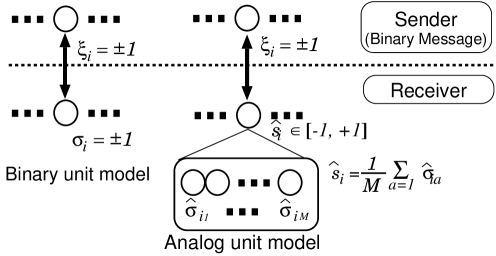
Figure 2: Analog model for analysis: In the binary model, encoding unit $\xi_{i}$ corresponds to decoding unit $\sigma_{i}$. In contrast, the analog model assumes a decoding unit has $M$ units, and the average of these $M$ units is regarded as the analog unit output.

where $\hat{s}_{i}$ denotes an output of an analog unit which takes a continuous value $[-1,+1]$ in the equilibrium state. $M$ is a scaling factor described below. To analyze the model described by the Hamiltonian Eq.(17), we followed the manner of Bray et al. Bray86 . We assumed each $i$th site consists of $M$ binary units, and the analog unit output $\hat{s}_{i}$ can be calculated using the average of $M$ binary units $\hat{\sigma}_{ia}$ (see Fig.2).

$$\hat{s}_{i}=\frac{1}{M}\sum_{a=1}^{M}\hat{\sigma}_{ia}$$ (18)

For the limit $M\rightarrow\infty$, each output $\hat{s}_{i}$ can take a continuous value $[-1,+1]$. When $M$ is a finite value, each $\hat{s}_{i}$ is called a ‘binominal spins’ which can take $-1,-1+\frac{2}{M},\cdots,1-\frac{2}{M},1$ with a binominal distribution. We can thus introduce a ‘spin weight function’ as

$$W(\hat{s}_{i}) =\>\>\mathrm{Tr}\>\>\delta\left(M\hat{s}_{i}-\sum_{a=1}^{M}\hat{\sigma}_{ia}\right)$$

$$=\frac{1}{2\pi{\mathrm{j}}}\int_{-{\mathrm{j}}\infty}^{+{\mathrm{j}}\infty}du_{i}\exp(M(-u_{i}\hat{s}_{i}+\ln 2\cosh(u_{i}))).$$ (19)

The partition function $\cal Z$ can be described as

$${\cal Z}=\prod_{i=1}^{N}\int_{-1}^{+1}d\hat{s}_{i}W(\hat{s}_{i})\exp(-\beta{\cal H})$$

$$=M\int_{-{\mathrm{j}}\infty}^{+{\mathrm{j}}\infty}\prod_{i=1}^{N}\left(\frac{du_{i}}{2\pi{\mathrm{j}}}\right)\int_{-1}^{+1}\prod_{i=1}d\hat{s}_{i}$$

$$\quad\quad\exp\Biggl{(}M\biggl{(}\beta\sum_{i_{1}<\cdots<i_{r}}J_{i_{1}\cdots i_{r}}\hat{s}_{i_{1}}\cdots\hat{s}_{i_{r}}$$

$$\quad+h\sum_{i}\tau_{i}\hat{s}_{i}-u_{i}\hat{s}_{i}+\ln 2\cosh(u_{i})\biggr{)}\Biggr{)}$$ (20)

At the limit $M\rightarrow\infty$, the integrals over $\{u_{i}\}$ and $\{\hat{s}_{i}\}$ in Eq. (20) can be evaluated by the saddle-point method. To derive the saddle-point equations, we differentiated the exponent of Eq.(20) by $\hat{s}_{i}$ and $u_{i}$, and obtained

$$0 =\frac{\beta}{(r-1)!}\sum_{i_{2}=1}^{N}\cdots\sum_{i_{r}=1}^{N}J_{i\>i_{2}\cdots i_{r}}\hat{s}_{i_{2}}\cdots\hat{s}_{i_{r}}+h\tau_{i}-u_{i},$$ (21)

$$0 =-\hat{s}_{i}+\tanh u_{i}.$$ (22)

To derive Eq.(21), we assumed $J_{i_{1}\cdots i_{r}}$ was symmetric:

$$J_{i_{1}\cdots i_{r}}=J_{i^{\prime}_{1}\cdots i^{\prime}_{r}},$$

where the indices group $(i^{\prime}_{1}\cdots i^{\prime}_{r})$ is any permutation group of $(i_{1}\cdots i_{r})$ . Moreover, we assumed self-coupled term in $J_{i_{1}\cdots i_{r}}$ equals zero:

$$J_{i_{1}\cdots l\cdots l\cdots i_{r}}=0.$$

Eliminating $u_{i}$ from Eqs.(21) and (22), we obtain

$$\hat{s}_{i} =\tanh\left(\frac{\beta}{(r-1)!}\sum_{i_{2}=1}^{N}\cdots\sum_{i_{r}=1}^{N}J_{i\>i_{2}\cdots i_{r}}\hat{s}_{i_{2}}\cdots\hat{s}_{i_{r}}+h\tau_{i}\right).$$ (23)

For example, for $r=3$, Eq.(23) can be denoted as

$$\hat{s}_{i}=\tanh\left(\frac{\beta}{2}\sum_{j=1}^{N}\sum_{k=1}^{N}J_{ijk}\>\hat{s}_{j}\hat{s}_{k}+h\tau_{i}\right),$$ (24)

where we assumed $J_{ijk}=J_{kij}=J_{jki}=J_{kji}=J_{ikj}=J_{jik}$, and $J_{ijj}=J_{jij}=J_{jji}=0$.

We can derive naturally a discrete synchronous updating rule:

$$s_{i}^{t+1}=\tanh\left(\frac{\beta}{(r-1)!}\sum_{i_{2},\cdots,i_{r}}J_{i\>i_{2}\cdots i_{r}}\hat{s}_{i_{2}}^{t}\cdots\hat{s}_{i_{r}}^{t}+h\tau_{i}\right).$$ (25)

where $s^{t}_{i}$ denotes the analog unit output at time $t$. Eq.(25) does not include any stochastic calculation, so we refer to Eq.(25) as the deterministic dynamics. When the model described by Eq. (25) reached to the equilibrium state $s^{\infty}_{i}$, all units should satisfy Eq. (23). Therefore, to investigate the equilibrium state of dynamics (Eq. (25)), we should use the analog Hamiltonian described by Eq.(17). From the idea of the NMF approximation, each analog unit state expressed by $s^{\infty}_{i}$ in the equilibrium state will correspond to $\langle\sigma_{i}\rangle$, i.e. $s^{\infty}_{i}$ can be regarded as the thermal average of $\sigma_{i}$. From Eq. (25), this model follows the deterministic dynamics, so there is no need to calculate the thermal average of a stochastic unit; the expected calculation cost is thus lower than that for the stochastic binary units model.

II.3 Equilibrium State Analysis

To investigate the macroscopic property, we analyzed the NMF approximated model that includes the Hamiltonian described by Eq. (17) through the “replica method”, which is a standard statistical-mechanical analysis tool. The MPM inference corresponds to the minimization of the free energy denoted as $T[\ln{\cal Z}]$. Here, ${\cal Z}$ is the partition function:

$${\cal Z}=\mathrm{Tr}_{\{\sigma_{ia}\}}\exp(-\beta{\cal H}),$$ (26)

where ${\cal H}$ is described as Eq.(17). However, it is impossible to evaluate $[\ln{\cal Z}]$ in practical, we use replica trick $[\ln{\cal Z}]=\lim_{n\rightarrow 0}([{\cal Z}^{n}]-1)/n$. The $n$ replicated partition function $[{\cal Z}^{n}]$ can be expressed as:

$$\left[{\cal Z}^{n}\right]=\mathrm{Tr}\left(\int\prod_{i_{1}<\cdots<i_{r}}\sqrt{\frac{N^{r-1}}{J^{2}\pi r!}}dJ_{i_{1}\cdots i_{r}}\right)\left(\int\prod_{i=1}\frac{1}{\sqrt{2\pi\tau^{2}}}d\tau_{i}\right)$$

$$\quad\quad\times P_{s}(\{\xi_{i}\})P_{{\mathrm{out}}}(\{J_{i_{1}\cdots i_{r}}\},\{\tau_{i}\}|\{\xi_{i}\}){\cal Z}^{n},$$ (27)

$${\cal Z}^{n}=\prod_{\alpha=1}^{n}\exp\biggl{(}\frac{\beta}{M^{r-1}}\sum_{i_{1}<\cdots<i_{r}}J_{i_{1}\cdots i_{r}}\sum_{k_{1},\cdots,k_{r}}\hat{\sigma}_{i_{1}k_{1}}^{\alpha}\cdots\hat{\sigma}_{i_{r}k_{r}}^{\alpha}$$

$$\quad\quad\quad+h\sum_{i}\tau_{i}\sum_{k}\hat{\sigma}_{ik}^{\alpha}\biggr{)},$$ (28)

where operator $\mathrm{Tr}$ in the last equation represents the sum over all states about $\{\hat{\sigma}_{ia}^{\alpha}\}$ and $\{\xi_{i}\}$. We analyzed this replicated partition function through the standard replica method. The replica symmetry solution can be described as

$$m =\int Dz\>G(z),$$ (29)

$$q =\int Dz\>G(z)^{2},$$ (30)

$$\chi =\frac{1}{\displaystyle\left(\frac{\beta^{2}J^{2}rq^{r-1}}{2}+h^{2}\tau^{2}\right)^{1/2}}\int Dz\>zG(z),$$ (31)

where

$$G(z)=\tanh\Biggl{(}\biggl{(}\frac{\beta^{2}J^{2}rq^{r-1}}{2}+h^{2}\tau^{2}\biggr{)}^{1/2}z$$

$$\quad+\frac{\beta^{2}J^{2}}{2}r(r-1)\chi q^{r-2}G(z)+\beta j_{0}rm^{r-1}+h\tau_{0}\Biggr{)}$$ (32)

Using these solutions, we could obtain the overlap $M_{o}$:

$$M_{o} =\left[\frac{1}{N}\sum_{i=1}^{N}\xi_{i}\>\mathrm{sgn}(\hat{s}_{i})\right]$$ (33)

$$=\int Dz\>\mathrm{sgn}\left(G(z)\right)$$ (34)

If we Assume $\chi=0$, this analysis agrees with the result obtained using stochastic binary units reported by Nishimori& Wong Nishimori00 . Thus, in our analysis, the difference in the result that arises from the reaction term $\frac{\beta^{2}J^{2}}{2}r(r-1)\chi q^{r-2}G(z)$ in Eq.(32).

Figure 3: Phase diagram of binary and analog models: The horizontal axis shows S/N ratio $j_{0}/J$, and the vertical axis shows the decoding temperature $T/J$. (a) shows the analysis result for the binary model, and (b) shows the result for the analog model. Region ‘F’ shows the retrievable area. (c) shows the difference between (a) and (b). Region ‘A’ is where the analog model is superior to the binary model and the region ‘B’ indicates the opposite.

III Result

In this section, we compare the theoretical and simulation results for the conventional stochastic binary model and the NMF approximated (deterministic analog) model. We refer to the decoding using the MPM inference with conventional stochastic binary units as the ‘binary model’ and to the NMF approximated model as the ‘analog model’. In subsection III.1, we show the analytical results for each model. In subsection III.2, we compare the results from these theoretical analyses with those from computer simulations. To compare these results, we configured an environment described by several parameters having the same value; that is, $r=3$, $h=0$, and $J=1$. The condition $r=3$ means a redundant message was generated by 3-body $\xi_{i}\xi_{j}\xi_{k}$ where $1\leq i<j<k\leq N$. We use $h=0$, which means the decoding was carried out using only information $\bm{J}$ corresponding to the redundant message. Thus, $\bm{\tau}$ had no effect in our decoding models. Under this condition, the original message was generated by uniform prior probability Eq.(2). The redundant messages were generated by Eq.(1), and the message corruption process is described by Eq.(4).

In the simulation, to decode the original message $\bm{\xi}$ from the corrupted signals $\bm{J}$ using the stochastic binary model, we used a kind of gradient descent algorithm –, that is Glauber dynamics, – to find the minimum state of the Hamiltonian $H$ described in Eq.(11). For decoding using the analog model, we used the update rule describe in Eq.(25) to find the minimum of the free energy of the Hamiltonian ${\cal H}$ described in Eq.(17).

III.1 The ability of NMF Approximation

Fig.3(a) is a phase diagram for the binary model with $r=3$. In the figure, we only show the ‘replica symmetry’ solution; a more detailed solution has been given by Nishimori & Wong Nishimori00 . The $x$-axis shows $j_{0}/J$, which corresponds to the S/N ratio in the communication channel, and the $y$ axis shows $T/J$, which corresponds to the decoding temperature. Region ‘F’, which represents the ferromagnetic state ($m>0$ and $q>0$), in the figure shows the retrievable region.

Fig.3(b) is a phase diagram for the analog model using the same parameters as for the binary model. Comparing figs.3(b) and 3(a), we see that the decoding ability of the analog model looks better than that of the binary model in the high temperature region.

In Fig.3(c), region “A” shows where the analog model is superior to the binary model, while region ‘B’ shows where the binary model provides better decoding ability than the analog model. The binary model is better when the S/N ratio is low, while the analog model is more robust with respect to the decoding temperature $T$.

III.2 Comparison with Computer Simulation

(a) Binary, $j_{0}/J=0.80$, $N=100$	(c) Binary, $j_{0}/J=1.0$, $N=100$
(b) Analog, $j_{0}/J=0.80$, $N=100$	(d) Analog, $j_{0}/J=0.80$, $N=100$

Figure 4: Comparison with Computer simulation. The error bars in each figure represent the computer simulation results. The horizontal axis shows the decoding temperature and the vertical axis shows the absolute value of the overlap $M_{o}$. Each error bar range represents the first and third quartile deviations, and the middle point indicates the median. The dashed line in each figure shows the replica analysis result.

The theoretical results described in sec.III.1, were realized in an equilibrium state, so we confirmed the validity of our theory through the computer simulations. In the simulations, we assumed a message length as $N=100$.

In the binary model simulation, we used asynchronous Glauber dynamics. First, we randomly selected one site $l$, and calculated the transition probability as determined by the heat-bath method:

$$W(\bm{\sigma}^{t}\rightarrow{\cal F}_{l}(\bm{\sigma}^{t}))=\frac{1}{1+\exp(\beta(H(\bm{\sigma}^{t})-H({\cal F}_{l}(\bm{\sigma}^{t}))))},$$ (35)

where the operator ${\cal F}_{l}(\cdot)$ flipped $\sigma_{l}^{t}$ to $-\sigma_{l}^{t}$. The difference of the Hamiltonian $H(\bm{\sigma}^{t})-H({\cal F}_{l}(\bm{\sigma}^{t}))$ can be denoted as

$$H(\bm{\sigma}^{t})-H({\cal F}_{l}\bm{\sigma}^{t})=2\sigma_{l}F_{l}(\bm{\sigma}^{t})$$ (36)

$$F_{l}(\bm{\sigma})=\frac{1}{(r-1)!}\sum_{i_{2},\cdots i_{r}}J_{li_{2}\cdots i_{r}}\sigma_{i_{2}}^{t}\cdots\sigma_{i_{r}}^{t}+h\tau_{l}$$ (37)

This is equivalent to determining the $l$th site probability by

$$P(\sigma_{l}^{t+1}=\pm 1)=\frac{1}{2}\pm\frac{\tanh(\beta F_{l}(\bm{\sigma}^{t}))}{2}.$$ (38)

In this simulation, the initial state $\bm{\sigma}^{1}$ was set to the true message $\bm{\xi}$, so the simulation result indicated the stability of the true message in the model.

In the analog model simulation we used the synchronous update rule describe in Eq..(25). Thus all units were updated simultaneously. In the analog simulation, we also set the true message $\bm{\xi}$ as the initial state $\bm{s}^{1}$.

Figs.4(a) and (c) show the binary model simulation results along with the theoretical analysis results at $j_{0}/J=0.8$ and $j_{0}/J=1.0$, respectively. (The horizontal axis shows $T/J$, and the vertical axis shows the absolute value of the overlap $|M_{o}|$.) The computer simulation results are represented by error bars showing the quartile deviation, and the dashed line shows the theoretical analysis result. The phase transition occurred at about $T/J=1.0$ and $T/J=1.5$ in figs.4(a) and (c), respectively, and the results of the computer simulation agree with the theoretical analysis results.

Figs.4(b) and (d) shows the analog model simulation results along with the theoretical analysis results at $j_{0}/J=0.8$ and $j_{0}/J=1.0$, respectively. The computer simulation results are again represented by error-bars, and agree with the replica analysis results. In figs.4(b) and (d), the theoretical results show that the phase transition occurred at about $T/J=1.5$ and $T/J=1.9$, respectively. The computer simulation agreed with the analysis at such high temperatures. In the analog model, the critical temperatures, which cause the phase transition, became higher than those of the binary model. This indicates that the deterministic analog decoding model is more robust than the binary decoding model in terms of decoding ability when the receiver overestimates the decoding temperature.

However, at low temperatures in the analog model the simulation results did not agree with theoretical result (Fig.4(b)). The simulation initial state is $\bm{s}^{1}=\bm{\xi}$, and there exist meta-stable states around the $\bm{\xi}$, so the dynamics of $\bm{s}^{t}$ is captured by this state and the absolute overlap $|M_{o}|$ stays close to $1.0$.

An important feature of the analog model simulation results shown in figs.4(b) and (d), is that the absolute value of the overlap $|M_{o}|$ was exactly $0$ at high temperature. In the analog model, the all units value $s_{i}$ exactly converged to $0$ for any messages $\{\bm{\xi}\}$, so we can guess whether the retrieval is failed or not at high temperature exceeding the retrievable limit. In practical, the ability to determine whether decoding will be finished in failure or success is a desirable feature.

III.3 Convergence Speed

Figure 5: Convergence of the macroscopic quantity $m(t)$: the solid line represents the analog model and the dashed line represents the binary model. $t_{\text{min}}=1$

The main advantage of the NMF approximation is the low calculation cost of convergence. Here, we discuss the convergence time that should be set in the computer simulation for each method. To calculate the thermal average in the computer simulation, we implemented

$$\overline{\langle\sigma^{t}_{i}\rangle} =\frac{1}{T}\sum_{\tau=t_{\text{min}}}^{t}\sigma_{i}^{\tau},$$ (39)

$$T =t-t_{\text{min}}+1,$$ (40)

as the thermal average, where the superscript $t$ means discrete time and $t_{\text{min}}$ means the beginning of thermal average calculation. First, we observed the macroscopic quantities $m^{t}$;

$$m^{t}=\left\{\begin{array}[]{ll}\frac{1}{N}\sum\overline{\langle\sigma^{t}_{i}\rangle}&\>\>\>{\text{(binary model)}}\\ \frac{1}{N}\sum s^{t}_{i}&\>\>\>{\text{(analog model: NMF approximation) }}\end{array}\right.$$ (41)

In this simulation, we set the initial value $\bm{s}^{1}$ and $\bm{\sigma}^{1}$ to satisfy the overlap $M_{o}=0.8$, and $t_{\text{min}}=1$. Fig.5 shows the dynamics of $m^{t}$. The solid line represents $m^{t}$ of the binary stochastic model and the dashed line represents that of the analog deterministic model. The convergence times for the two lines seem to be of the same order.

(a)	(b)

Figure 6: Typical dynamics of $\overline{\langle\sigma_{1}^{t}\rangle}$ and $s_{1}^{t}$. The solid lines show the dynamics of $s^{t}_{1}$ which converged within $t_{\text{min}}=100$ iterations. The dashed lines show the dynamics of $\overline{\langle\sigma_{1}^{t}\rangle}$. In (a), the S/N ratio and temperature parameters were set to $j_{0}/J=1.0$ and $T/J=1.0$, respectively. The convergence of $\overline{\langle\sigma_{1}^{t}\rangle}$ was slower than that of $s^{t}_{1}$. In (b), the temperature was set to $T/J=1.80$; i.e., outside of the retrieval region. In this case the convergence of $\overline{\langle\sigma_{1}^{t}\rangle}$ was also slow.

In the MPM inference, however, we should determine each unit’s value; that is, the microscopic quantity. Thus, we investigated the behavior of the thermal average of unit $\overline{\langle\sigma_{1}^{t}\rangle}$ for the binary model and $s_{1}^{t}$ for the analog model. In the analog model, all units were updated simultaneously because we adopted synchronous updating. In contrast, we adopt asynchronous updating in the binary model. To compare the convergence time between analog unit and binary unit, we regarded $N$ updates as one Monte Carlo step ($1$ MCS) for binary model, where $N(=100)$ means the number of units in the simulation. Thus, one MCS update corresponds to one synchronous update in the analog model. Fig. 6(a) shows a typical result regarding the convergence speed for the S/N ratio $j_{0}/J=1.0$ and temperature $T/J=1.0$; we set the beginning of the thermal average calculation as $t_{\text{min}}=100$ MCS. The horizontal axis shows the calculation time measured by MCS, and the vertical axis shows the value of $\sigma_{1}^{t}$ and $s_{1}^{t}$. The solid line shows typical dynamics of $\sigma_{0}^{t}$, and the dashed line shows typical dynamics of $s_{0}^{t}$. In macroscopic points of view, each model achieved the same overlap $|M_{o}|$, but in microscopic perspective, the deterministic analog model converged about over 1000 times as quickly as the stochastic binary model.

Fig. 6(b) shows the dynamics at a higher temperature $T/J=2.2$. $\overline{\langle\sigma^{t}_{1}\rangle}$ did not converge to 0; however $s_{1}^{t}$ seemed to be converging to exactly $0$ in the early time steps. Thus, when using the analog model, we can easily predict within the early time steps whether the decoding will be finished in failure or not.

IV Conclusion

In this research, we have investigated an error-correcting code that uses the MPM inference. Since the MPM inference requires many trials to calculate the thermal average for each unit, we tried to replace this operation with a form of deterministic analog dynamics called naive mean field approximation. We analyzed the decoding ability with the deterministic analog model through the replica method, and quantitatively compared it with that of the stochastic binary model suggested by Nishimori & WongNishimori00 . We found that the decoding ability of the deterministic analog model is superior to that of the stochastic binary mode l at higher temperature area. To confirm this result, we carried out a computer simulation for each model and obtained the results that agreed with our analysis results.

References

- (1) D. C. Mattis. Solvable spin systems with random interactions. Physics Letter A, 56A(5), April 1976.
- (2) C.E. Shannon. A Mathematical Theory of Communication. Bell System Technical Journal, 27:379–423, 623–656, 1948.
- (3) Y. Kabashima and D. Saad. Belief Propagation vs. TAP for decoding corrupted messages. EuroPhys.letter, 44(5):668–674, 1999.
- (4) P. Ruján. Finite Temperature Error-Correcting Codes. Physical Review Letters, 70(19):2968–2971, 1993.
- (5) N. Sourlas. Spin Glasses, Error-Correcting Codes and Finite-Temperature Decoding. Europhysics Letters, 25(3):159–164, 1994.
- (6) H. Nishimori and K. Y. M. Wong. Statistical mechanics of image restoration and error-correcting codes. Physical Review E., 60(1):132–144, 1999.
- (7) A. J. Bray, H. Sompolinsky, and C. Yu. On the ‘Naive’ Mean-Field Equations for Spin Glasses. J.Phys.C: Soliid State Phys., 19:6389–6406, 1986.
- (8) J. J. Hopfield and D. W. Tank. Computing with neural circuits: A model. Science, 233:625–633, 1986.
- (9) H. Shouno, K. Wada, and M. Okada. Naive mean field approximation for image restoration. Journal of Physical Society Japan, 71(10), Oct. 2002.
- (10) M. Vecchi. S. Kirkpatrick, C. Gelatt. Optimization by simulated annealing. Science, 220(4589):671–680, 1983.