From Bubble to Skyrmion: Dynamic Transformation Mediated by a Strong Magnetic Tip

Abstract

Skyrmions in thin metallic ferromagnetic films are stable due to competition between the RKKY interaction and uniaxial magnetic anisotropy. We mimic the RKKY interaction by the next-nearest-neighbors ferromagnetic and antiferromagnetic exchange interactions. We demonstrate analytically and numerically dissipative transformation of a bubble created by a strong cylindrical magnetic tip into a stable Skyrmion.

I Introduction

Recently a significant progress has been achieved in the nanofabrication and design of new technologies for very high density storage on hard disks (densities above 500 Gbit/in² ) kirk&all00 and magnetoresistive random access memory (MRAM). For the further miniaturization of the data storage and the magnetic memory it is important to decrease the size of nanoelements. Magnetic defects in such nanoelements storing bits of information can have very small size. The properties of Skyrmion in thin metallic magnetic films (the small size about 1 nm and stability) may allow to use their two-dimensional (2D) arrays in magnetic storage devices. To the best of our knowledge a magnetic memory based on Skyrmions was not developed yet. There are no analogs of storage of so extremely high density.

Skyrmions are strongly localized scale invariant analogs of magnetic bubble domains (MBD) bubble . The axially symmetric Skyrmion solution for boson fields minimizing the Hamiltonian and describing the structure of nuclear matter was first found by Skyrme Skyrm58 . Belavin and Polyakov based on nonlinear $\sigma$-model have established that Skyrmion is a topologically nontrivial metastable minimum of energy BP75 . Since then the properties of Skyrmions in two-dimensional magnets and thin magnetic films have been widely investigated in last few decades voronov&all83 ; ivanov&all90 ; Abanov&Pokrovsky98 ; abdullaev&all99 ; sheka&all01 .

Slow relaxation spin dynamics of Skyrmion was studied by Abanov and Pokrovsky Abanov&Pokrovsky98 . They calculated the radius of the Skyrmion as a function of time. They have found that the interaction of the Ruderman-Kittel-Kasuya-Yosida (RKKY) type together with the uniaxial magnetic anisotropy can stabilize the Skyrmion.

In quasi-2D antiferromagnets the Skyrmions were indirectly observed by F. Waldner by the ESR waldner83 and the heat capacity measurements waldner86 in a good agreement with the Belavin and Polyakov (BP) theory. The appearance of Skyrmions in the QHE was predicted by Sondhi et al. sondhi&al93 . In the regime of fractional QHE Skyrmions were discovered experimentally in GaAs quantum wells by means of optically pumped NMR and by measurements of the Knight shift, which is proportional to the electron magnetization barrett&all95 . For integer QHE Skyrmions were detected in thermal magnetotransport measurements schmeller95 and in optical absorption aifer96 .

Recently another topological excitations, magnetic vortices were observed and studied experimentally in permalloy and Co nanodisks by means of the Lorentz microscopy and Magnetic Force Microscopy (MFM) schneider&all00 . The evolution and stability of such magnetic vortices in a small isotropic cylindrical magnetic dot was analyzed theoretically in guslienko&metlov01 .

The equilibrium size of Skyrmion in 2D thin magnetic films is extremely small. This is one of serious obstacles for its experimental observation. For soft magnets the size of vortices is defined by competition between the exchange and magnetic dipole interaction. In uniaxial magnets, strong uniaxial anisotropy together with the fourth order exchange interaction leads to small size of Skyrmion. Recent great progress in nanotechnology gives a chance to detect experimentally Skyrmions in thin magnetic films. The experimental methods employed for studying Skyrmions in QHE systems and vortices in soft magnetic dots can be also applied to 2D uniaxial magnets. So far the only technique potentially capable of atomic resolution is the spin-polarized scanning tunneling microscopy (SPSTM).

Due to stability of the Skyrmion in an uniaxial thin metallic magnetic film it is possible to create it by a strong magnetic tip. In this paper we study the properties of the MBD created by the tip as well as its relaxational dynamics when tip moves away uniformly and vertically from the film. When the distance between the film and the tip exceeds a critical value, it is not able to confine the MBD anymore and the latter collapses and gradually transforms into a stable Skyrmion. For numerical simulations we use a stabilization mechanism provided by the interplay between next nearest neighbor antiferromagnetic interaction and the magnetic anisotropy. We also show that the demagnetization energy of the Skyrmion is equivalent to the renormalization of the single ion anisotropy constant. We find that demagnetizing field produced by a single Skyrmion is strongly localized around Skyrmion center.

The plan of this paper is as follows. In Section II we introduce a theoretical model and equations of motion. We calculate the demagnetization energy of the Skyrmion in Section 1. Section IV is devoted to the magnetic field generated by a cylindrical tip. In Section V we study static properties of the MBD and the Skyrmion solving numerically Landau-Lifshitz equation with the fitting method. In Section VI we study analytically and numerically a discrete spin model with the dipolar interaction and find stability condition for the static Skyrmion. Relaxational dynamics of the transformation of a MBD into a Skyrmion in the presence of an uniformly moving tip is considered in Section VII. Our conclusions and discussions are presented in the last section VIII.

II Model

We consider the two-dimensional Heisenberg model with the exchange interaction up to the fourth order derivatives and uniaxial anisotropy in continuous approximation. Its Hamiltonian has a following form

$${\cal H}=h\int W({\bf M})\,d^{2}x$$ (1)

where $W({\bf M})=W_{e}({\bf M})+W_{a}({\bf M})+W_{Z}({\bf M})$ and

$$W_{e}({\bf M}) = {\alpha\over 2}\left((\nabla{\bf M})^{2}+{a^{2}\kappa\over 2\,M_{0}^{2}}(\nabla{\bf M})^{4}\right)$$ (2)

$$W_{a}({\bf M}) = {\beta\over 2}(M_{0}^{2}-M_{z}^{2}),$$ (3)

$$W_{Z}({\bf M}) = H_{z}\,M_{0}-\left({\bf H}(r,d(t))+{1\over 2}{\bf H^{D}}\right)\,{\bf M},$$ (4)

Here the energy density $W({\bf M})$ consists of the exchange energy $W_{e}({\bf M})$, the uniaxial anisotropy energy $W_{a}({\bf M})$; $W_{Z}({\bf M})$ contains the interaction energy of cylindrical tip with the magnetic film and the demagnetization energy. In our notations $\alpha$ is the exchange interaction constant, $\beta$ is the easy-axis anisotropy constant, $\kappa$ is a positive dimensionless constant, characterizing the fourth order exchange interaction (we consider just this term because of its simplicity), $M_{0}$ is the spontaneous magnetization of the film, ${\bf H}(r,d)$ is the magnetic field created by the magnetic tip (cylinder) at the surface of the film as a function of the polar radius $r$ and the distance $d$ between the cylinder and the plane of the film; $h$ is the film thickness. In a thin magnetic film the demagnetization energy of a localized magnetic excitation with the radius $R_{e}$ at $R_{e}\ll h$ simply renormalizes the anisotropy constant $\beta$ ($\beta\rightarrow\beta-4\pi$). In the opposite case $R_{e}>h$ the demagnetization energy is more complicated. Below we calculate it for the Skyrmion. For iron the exchange length $l_{ex}=1.5nm$. Therefore, an ultrathin iron film consists of few monolayers.

The dynamics of a classical 2d ferromagnet is governed by the Landau-Lifshitz equation (LLE) for the magnetization vector ${\bf M}$

$$\dot{\bf M}({\bf r},t) = \gamma\,{\bf M}({\bf r},t)\times\frac{\delta{\cal H}[{\bf M}]}{\delta{\bf M}({\bf r},t)}+$$

$${\Gamma\,\dot{\bf M}({\bf r},t)\times{\bf M}({\bf r},t)\over M_{0}}$$ (5)

here $\gamma=g\mu_{B}/\hbar$; $g$ and $\mu_{B}$ are the gyromagnetic ratio and the Bohr magneton, respectively, and $\Gamma$ is the dimensionless Gilbert damping constant. The LLE equation (5) in angular variables $\theta$ and $\phi$ can be derived from the Lagrange-Hamilton variational principle with the following Lagrangian density ${\cal L}(\theta,\phi)$

$${\cal L}(\theta,\phi)={M_{0}\over\gamma}\,(1-\cos\theta)\,{\partial\phi\over\partial t}-W(\theta,\phi)$$ (6)

In the static case the LLE Eq. (5) read:

$$M_{0}^{2}\,{\delta{\cal H}\over\delta{\bf M({\bf r})}}={\bf M({\bf r})}\,\left({\bf M({\bf r})}\cdot{\delta{\cal H}\over\delta{\bf M({\bf r})}}\right)$$ (7)

The right-hand side of Eq. (7) originates from a constraint: ${\bf M}^{2}=M_{0}^{2}$ at any point ${\bf r}$.

The classical ground state is double degenerate due to uniaxial magnetic symmetry. A topologically nontrivial minimum of the Hamiltonian (1) corresponds to the Skyrmion solution

$$M^{s}_{x} = M_{0}\,{2\,R_{s}\,r\over R_{s}^{2}+r^{2}}\cos(\varphi+\psi),$$

$$M^{s}_{y} = M_{0}\,{2\,R_{s}\,r\over R_{s}^{2}+r^{2}}\sin(\varphi+\psi),$$

$$M^{s}_{z} = M_{0}\,{r^{2}-R_{s}^{2}\over r^{2}+R_{s}^{2}}.$$ (8)

The Skyrmion is characterized by its radius $R_{s}$ and an angle $\psi$ of the global spin rotation; $r$ and $\varphi$ are polar coordinates. For isotropic magnets the energy of Skyrmion does not depend neither on $R_{s}$ nor on $\psi$. In real systems the degeneracy with respect to $R_{s}$ is lifted by uniaxial magnetic anisotropy and by the fourth order exchange interaction.

Another static solution of the LLE is the well known MBD, which was the subject of intensive study during last few decades. Here we consider an MBD with the topological charge one. The structure of such a soliton can be approximately described by the ”domain-wall” ansatz:

$$M^{b}_{x} = M_{0}\,\mbox{sech}{r-R_{b}\over l_{0}}\cos(\varphi+\psi),$$

$$M^{b}_{y} = M_{0}\,\mbox{sech}{r-R_{b}\over l_{0}}\sin(\varphi+\psi),$$

$$M^{b}_{z} = M_{0}\,\tanh{r-R_{b}\over l_{0}},$$ (9)

where $R_{b}$ is the MBD radius. Since we consider an ultrathin magnetic film, the MBD exists only in the presence of an external magnetic field and collapses without this field.

III Demagnetization fields

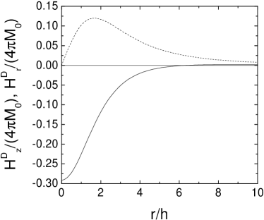
Figure 1: Demagnetizing field of the Skyrmion (13) versus polar radius normalized to the film thickness $r/h$. Solid and dashed lines correspond to $H^{D}_{z}/(4\pi M_{0})$ and $H^{D}_{r}/(4\pi M_{0})$, respectively. The radius of Skyrmion $R_{s}=2h$.

Let us now return to the demagnetization energy. The magnetostatic problem for the non-topological MBD was solved first by Thiele thiele69 ; thiele70 . He expressed ${\cal H}_{D}$ in terms of elliptic integrals. The Thiele’s solution for demagnetizing field $x^{-1}(\partial{\cal E}_{D}/\partial x)$ can be approximated with surprisingly good accuracy by callen&josephs71

$$x^{-1}(\partial{\cal E}_{D}/\partial x)\approx-(1+3x/2)^{-1},$$ (10)

where dimensionless radius $x=R_{b}/h$ and dimensionless energy ${\cal E}_{D}=(16\pi^{2}M_{0}^{2}h^{3})^{-1}{\cal H}_{D}$ are introduced. For magnetostatic interaction the topological charge does not play any role. Hence the Thiele’s solution persists when dipolar forces are taken in account.

For ultrathin magnetic films consisting of few layers the ratio of the exchange length to the thickness is $l_{ex}/h>4/3$. Therefore, the MBD solution is unstable without external magnetic field.

The reading of the information stored by Skyrmions can be performed by the measurement of the Skyrmion magnetic field. Below we calculate this field and its energy. The Fourier transform of the Skyrmion magnetic field has the following form

$${\bf h}^{D}({\bf k})=-4\pi\,{\bf k}\,{({\bf k}\cdot{\bf m}({\bf k}))\over{\bf k}^{2}}$$ (11)

The magnetostatic energy in terms of the magnetization Fourier-components reads:

$${\cal E}_{D}={1\over(2\pi)^{2}}\int{\mid{\bf k}\cdot{\bf m}({\bf k})\mid^{2}\over{\bf k}^{2}}d{\bf k}$$ (12)

To calculate the magnetic field we substitute the Fourier transform of the Skyrmion magnetization (8) into (11) and perform the inverse Fourier transformation. The result is as follows:

$$H^{D}_{z}=4\pi M_{0}\,R_{s}^{2}\int_{0}^{\infty}F_{z}(q,z,h)\,K_{0}(qR_{s})\,J_{0}(qr)\,qdq$$

$$-4\pi M_{0}\Theta[h/2-|z|]$$

$$H^{D}_{r}=4\pi M_{0}\,R_{s}^{2}\int_{0}^{\infty}F_{r}(q,z,h)\,K_{0}(qR_{s})\,J_{1}(qr)\,qdq,$$ (13)

where

$$F_{z} = \mbox{sign}\left({h\over 2}-z\right)\,e^{-q\left|{h\over 2}-z\right|}+\mbox{sign}\left({h\over 2}+z\right)\,e^{-q\left|{h\over 2}+z\right|}$$

$$F_{r} = e^{-q\left|{h\over 2}-z\right|}-e^{-q\left|{h\over 2}+z\right|},$$ (14)

The origin of the frame of reference coincides with the Skyrmion center. The Skyrmion demagnetizing field for $R_{s}/h=2$ is shown in Fig. 1. The demagnetization energy of the Skyrmion (12)in units $E_{0}$ has the following form:

$${\cal E}_{D}={\cal E}_{D}^{1}-{4\pi\over\beta}\,{\cal E}_{an},$$ (15)

where the last term is a part of magnetostatic energy renormalizing anisotropy constant: $\beta\rightarrow\beta-4\pi$ ivanov&all90 and ${\cal E}_{D}^{1}$ has the form

$${\cal E}_{D}^{1} = {\pi\rho^{3}\over 8}\left(3\pi-4E\left(m\right)-2K\left(m\right)\right)$$ (16)

$$-{1\over 18}\,{{}_{p}F_{q}}\left(\{1,1,3\},\{{5/2},{5/2}\},m\right)$$

$$+{\rho^{2}\over 2}\,{{}_{p}F_{q}}\left(\{1,1,1\},\{{3/2},{3/2}\},m\right),$$

where $\rho=R_{s}/h$, $m=1/(4\rho^{2})$, $K(m)$ and $E(m)$ are the complete elliptic integrals of first and second kind, respectively, and ${{}_{p}F_{q}}(\{a_{1},\ldots,a_{p}\},(\{b_{1},\ldots,b_{q}\},m)$ is the generalized hypergeometric function. We consider ultrathin film $\rho\geq 1$. Employing an appropriate expansions for the elliptic integrals and hypergeometric functions we find

$${\cal E}_{D}^{1}\approx{\rho^{2}\over 2}+{\pi^{2}\,\rho\over 128}-{26\over 225}-{1\over 150\rho^{2}};\qquad\rho\gg 1$$ (17)

The expression (17) can be replaced by $\rho^{2}/2+\pi^{2}\,\rho/128$ in the interval $\rho>1$ with the accuracy of half percent.

The spin - polarized scanning tunneling microscopy (SP-STM) and spectroscopy (SP-STS) offers a great potential to unravel the structure of a single Skyrmion and Skyrmion arrays on the nanometer scale.

IV Cylindrical magnetic tip

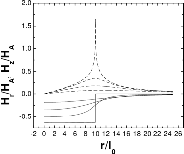
Figure 2: Components of the magnetic field of the tip (18) and (19) at a distance $d$ from the film: $d/l_{0}$ 0, 2, 5 and 10. $H_{A}=\beta M_{0}$ is the anisotropy field of the film and $l_{0}=10\,nm$ is the magnetic length. Solid and dashed lines correspond to $H_{z}$ and $H_{r}$ components, respectively. The radius of magnetic tip $R=10\,l_{0}=100\,nm$, the ratio of magnetization of the tip to that of the film is $M_{t}/M_{0}=10$.

Consider a semi-infinite cylindrical magnetic tip. The stray magnetic field of the cylindrical tip is well known. Its $z$ and $r$ components are

$$H_{z}(r,d) = -2\pi M_{t}R\int_{0}^{\infty}dq\,J_{1}(qR)\,J_{0}(qr)\,e^{-qd},$$ (18)

$$H_{r}(r,d) = 2\pi M_{t}R\int_{0}^{\infty}dq\,J_{1}(qR)\,J_{1}(qr)\,e^{-qd},$$ (19)

where $M_{t}$, $R$ and $d$ are the magnetization, the radius of cylinder and the distance between the tip and magnetic film plane respectively. The radial component of the magnetic field of the tip $H_{r}(R,d)$ at the edge $r=R$ can be expressed in terms of the hypergeometric function:

$$H_{r}(R,d)=\pi\,M_{t}\,{R^{3}\over d^{3}}\,_{2}F_{1}\left({3\over 2},{3\over 2},3,-{4R^{2}\over d^{2}}\right),$$ (20)

This value diverges logarithmically when the distance between the tip and the magnetic film approaches zero:

$$H_{r}(R,d)\approx M_{t}\,\left\{\begin{array}[]{ll}2\,\mbox{ln}\left({8R\over e^{2}d}\right)&d\ll R\\ &\\ {\pi\,R^{3}/d^{3}}&d\gg R\end{array}\right\}$$

In a special case when the distance between the film and the tip $d=0$ the components of the magnetic field are:

$$H_{z}(r) = -2\,\pi M_{t}\,\Theta[R-r],$$ (21)

$$H_{r}(r) = \pi M_{t}\,\left({r\over R}\right)^{\sigma}\,_{2}F_{1}\left({1\over 2},{3\over 2},2,\left({r\over R}\right)^{2\sigma}\right),$$ (22)

where $\sigma=\mbox{sign}(R-r)$ and $\Theta$ is the Heaviside function. The expression (22) logarithmically diverges at the distances close to the tip’s edge $r=R$

$$H_{r}(r)\approx 2\,M_{t}\mbox{ln}\left(\ {8R\over e^{2}|r-R|}\right)$$ (23)

The components of magnetic field of the tip versus $r$ at different $d$ are depicted in Fig. 2.

At large distances $r\gg R$ the magnetic tip is equivalent to a magnetic charge $Q=M_{t}\pi R^{2}$ and asymptotically the magnetic field is Coulomb-like:

$$H_{z}(r,d) = -{\pi M_{t}R^{2}d\over(r^{2}+d^{2})^{3/2}},$$ (24)

$$H_{r}(r,d) = {\pi M_{t}R^{2}r\over(r^{2}+d^{2})^{3/2}},$$ (25)

To make tip stronger by increasing magnetic charge of the tip $Q$ it is possible to increase the radius of the tip or its magnetization. The first method is more effective.

V Static excitations in the presence of the tip

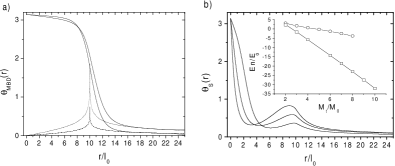
Figure 3: Profile of $\theta(r)$ at $d=0$ and different values of the ratio of the tip magnetization to that of the film $M_{t}/M_{0}$. a) Profile of $\theta_{MBD}$ for $M_{t}/M_{0}=4,10$. The radial component of magnetic field is shown on the same figure. b) A Skyrmion-like solution strongly distorted by the cusp of $H_{r}$ at the edge of the tip at $M_{t}/M_{0}=5,7,8$. The energies of MBD $\square$ and Skyrmion $\bigcirc$ versus $M_{t}/M_{0}$ are shown in insert. $E_{0}=4\pi\alpha hM_{0}^{2}$ is the energy of the unperturbed Skyrmion.

In order to study the relaxation dynamics of the Skyrmion created by the magnetic tip it is necessary first to analyze static solutions of the LLE for the magnetic film. A rough estimate of the minimal tip radius stabilizing the MBD at very small distance $d$ can be extracted from the balance of energy: $R_{0}=\varepsilon_{dw}/(2\pi M_{t}M_{0})$, where $\varepsilon_{dw}=2\sqrt{\alpha\beta}M_{0}^{2}$ is the linear tension of the domain wall. For more accurate analysis the knowledge of the magnetization and magnetic field distribution is necessary.

Several cylindrically symmetric soliton-like solutions of the LLE have been found. They are the static Skyrmion solution ivanov&all90 ; Abanov&Pokrovsky98 , the dynamic Skyrmion with the spin precession abdullaev&all99 and the slowly precessing magnetic bubble domain (MBD) sheka&all01 .

The precessing solitons can live longer than solitons without precession, though they finally also collapse due to dissipation, in accordance with the Derick-Hobart theorem hobart63 ; derrick64 . The collapse does not proceed if the Skyrmion configuration is stabilized by the higher order exchange interaction. Stabilization also occurs in ferromagnets without center of inversion ivanov&all90 .

Let us rewrite the LLE in terms of spherical coordinates $\theta$ and $\phi$, which determine the direction of magnetization:

$${1\over\omega_{0}}\sin\theta\,\dot{\theta}=l_{0}^{2}\,\mbox{div}\left(\sin^{2}\theta\,\nabla\phi\left(1+a^{2}\kappa\,(\nabla{\bf m})^{2}\right)\right)-{gH_{r}\over\omega_{0}}\sin\theta\,\sin(\phi-\varphi)-{\Gamma\over\omega_{0}}\dot{\phi}\,\sin^{2}\theta,$$ (26)

$${1\over\omega_{0}}\sin\theta\,\dot{\phi}=l_{0}^{2}\,\left(-\nabla^{2}\theta+(\nabla\phi)^{2}\sin\theta\cos\theta\right)(1+a^{2}\kappa(\nabla{\bf m})^{2})-l_{0}^{2}\,a^{2}\,\kappa\,\mbox{div}((\nabla{\bf m})^{2})+$$

$$\sin\theta\,\cos\theta+\,{gH_{z}\over\omega_{0}}\,\sin\theta-{gH_{r}\over\omega_{0}}\,\cos\theta\,\cos(\phi-\varphi)+{\Gamma\over\omega_{0}}\dot{\theta},$$ (27)

where $(\nabla{\bf m})^{2}=(\nabla\theta)^{2}+\sin^{2}\theta\,(\nabla\phi)^{2}$, $\varphi$ is the azymuthal angle in the film plane; $l_{0}=\sqrt{\alpha/\beta}$ is the magnetic length and $\omega_{0}=\beta gM_{0}$ is the ferromagnetic resonance frequency. In the static solution $\phi=\varphi$ and $\theta(r)$ obeys an ordinary differential equation:

$${d^{2}\theta\over dr^{2}}+{1\over r}{d\theta\over dr}-\sin\theta\cos\theta\left({1\over l_{0}^{2}}+{1\over r^{2}}\right)+$$

$$a^{2}\kappa\left({1\over r}{d\over dr}\left(r\,(\nabla{\bf m})^{2}{d\theta\over dr}\right)-{\sin\theta\cos\theta\over r^{2}}(\nabla{\bf m})^{2}\right)-h_{z}\sin\theta+h_{r}\cos\theta=0,$$ (28)

where $h_{z,r}=H_{z,r}/\alpha M_{0}$. Equation (28) should be solved with the following boundary conditions: $\theta(0)=\pi$, $\theta(\infty)=0$.

One of the most powerful tools to solve the nonlinear ordinary differential equations is the fitting method. The heart of this method is the matching of a numerically derived solution to a known asymptotics at small and large distances from the center of nonlinear excitation by varying the shooting parameter.

The key problem in this method is to find a proper trial function, with known asymptotics at $r\rightarrow 0$ and $r\rightarrow\infty$ and fits it to the asymptotics of the real solution. We solve LLE for $\theta(r)$ (28) by the fitting method. We choose the trial function $\theta(r)$ in the following form:

$$\tan{\theta^{(f)}\over 2}={R^{(f)}\over r}\exp\left[-{(r-R^{(f)})\over l_{0}}\right].$$ (29)

The trial function (29) has two advantages. First, it interpolates between two principal magnetic textures: the MBD and the Skyrmion by varying the fitting parameter $R^{(f)}$, and second, it has a valid asymptotic at $r\rightarrow 0$. Being distorted by the radial component of the tip magnetic field $H_{r}$, the radial component of the magnetization acquires an unusual power asymptotics $\sim 1/r^{2}$. This behavior is more pronounced when the tip is close to the magnetic film ($d\ll R$). In this case the radial component of the tip magnetic field cannot be treated as a perturbation, since it causes a strong distortion of the Skyrmion. Small and large values of $R_{f}$ correspond to the Skyrmion solution (8) and the MBD, respectively. We match the numerical solutions of LLE with the known asymptotic at infinity.

Let us now consider a special case when the distance between the surface of the and the tip $d$ is zero. The angle $\theta(r)$ at large distances decreases as $1/r^{2}$, similarly to $h_{r}$. At small distances, the solution for $\theta$ has the Skyrmion asymptotic. We have solved numerically equation (28) for $\theta$ with the shooting method for different $\mu=M_{t}/M_{0}$. For each value of $\mu$ we have found two different values of the fitting parameter $R_{f}$ satisfying the matching condition. We treat the solution with larger $R_{f}$ as the MBD, whereas the solution with smaller $R_{f}$ is interpreted as the Skyrmion-like solution. Profiles of $\theta(r)$ for different values of $\mu$ are presented in Fig. 3. The cusp of $h_{r}$ component of the magnetic field of the tip produces the noticeable distortion of Skyrmion solution in the region of the tip’s edge. This distortion grows with $\mu$ increasing as it is seen from Fig. 3. Strongly distorted Skyrmion-like excitation is the second solution of Landau-Lifshitz equation, but its energy is larger than that of the MBD. Thus, the magnetic tip nucleates MBD at static conditions. Fig. 3 illustrates that the radius of the generated MBD equals roughly to the radius of the tip. This result can be obtained banalytically by the direct minimization of energy.

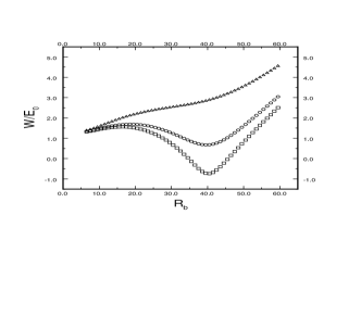
Figure 4: The normalized energy of the MBD $W/E_{0}$ (31) as a function of MBD radius $R_{b}$ at different distances between the tip and film. Curves with $\square$, $\bigcirc$ and $\bigtriangleup$ correspond to $d/R$ = 0.1, 0.2, 0.5 respectively. The ratio of the radius of the tip to the magnetic lenth $R/l_{0}=6$ and $\mu=5$.

In order to calculate the tip-film interaction energy we substitute the expressions (19) for $H_{z}$ and $H_{r}$ and equation (9) into (1). Using approximate relations: $\mbox{sech}^{2}\left((r-R_{b})/l_{0}\right)=2\,l_{0}\,\delta(r-R_{b})$ and $\mbox{sech}\left((r-R_{b})/l_{0}\right)=\pi\,l_{0}\delta(r-R_{b})$, we find

$$w_{Z}\equiv{W_{Z}\over E_{0}}=-\int_{0}^{\infty}k(q)\,J_{1}(qR)\,J_{1}(q\,R_{b})e^{-q\,d}\,dq,$$ (30)

where $k(q)={2\,\pi\mu R\,R_{b}\left({1/q}+{\pi\,l_{0}/2}\right)/(\beta\,l_{0}^{2})}$, $E_{0}$ is the unperturbed Skyrmion energy: $E_{0}=4\pi\alpha M_{0}^{2}$; and $\mu=M_{t}/M_{0}$. The total energy of the MBD $w$ in units $E_{0}$ is represented by the sum of 4 terms

$$w=w_{E}+w_{a}+w_{Z}+w_{D},$$ (31)

where $w_{E}$, $w_{a}$, $w_{Z}$ and $w_{D}$ are the exchange, the anisotropy, Zeeman and demagnetization energies, respectively. The partial sum $w_{E}+w_{a}$ can be represented by an interpolation formula:

$$w_{E}+w_{a}={R_{b}\over l_{0}}+0.5\,{l_{0}\over R_{b}},$$ (32)

valid with good precision in a broad interval of the ratio $R_{b}/l_{0}>2$. The first term in equation (32) is the linear tension of the domain wall, the second is the correction to it due nonzero topological charge of the MBD. The Zeeman energy is given by eq. (30). The demagnetizing energy $w_{D}$ for an ultrathin magnetic film ($h\ll l_{0}$) slightly renormalizes the exchange energy and can be neglected in the first approximation. This approximation is correct provided the radius of the MBD is much larger than the thickness of the film.

The energy of MBD versus its radius $R_{b}$ for different $d$ is shown in Fig. 4. If $d>d_{c}=0.385\,R$, the energy minimum at $R_{b}=R$ disappears; the tip cannot confine MBD anymore and the latter shrinks.

Accepting $R_{b}=R$, we find from Eq. (31) the range of parameters, in which the nucleation of the MBD is favorable:

$${R\over l_{0}}>{1-0.5\,\pi\,\xi\,g(p)\over\xi\,f(p)},$$ (33)

where $\xi=\pi\mu/\beta$,

$$g(p)=\,_{2}F_{1}\left({3\over 2},{3\over 2},3,-{4\over p^{2}}\right)/p^{3},$$ (34)

$$f(p)=1-{2p\over\pi\sqrt{k}}\left[K(k)-E(k)\right]$$ (35)

$p=d/R$, $k=(1+p^{2}/4)^{-1}$; $K(k)$ and E(k) are the complete elliptic integrals of the first and second kind, respectively.

The total energy of the MBD has the following form

$$w=\zeta+0.5/\zeta-\xi\,\zeta^{2}\,f(p)\,\cos\psi-0.5\pi\,\xi\,\zeta\,g(p),$$ (36)

where $\zeta=R_{b}/l_{0}$ and $\psi$ is the global rotation angle. In the equlibrium state $\psi=0$.

At a fixed radius of the tip $R$, the bubble nucleates when the distance between the tip and the film becomes less than some critical value $d_{c}$.

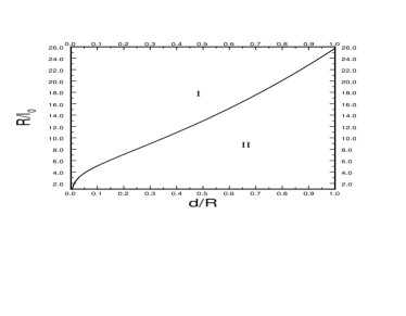
Figure 5: The phase diagram showing the range of parameters in which the nucleation of the MBD is energy favorable (region I). $d$ is the distance between the tip and the surface of the film; $R$ is the tip radius, $\mu=5$, $\beta=100$.

VI Discrete spin model with the dipolar interaction

In this section we study the dynamics of the bubble creation and its transformation into a stable Skyrmion solving numerically time-dependent Landau-Lifshitz equation on a discrete lattice. We employ the model of a classical two-dimensional Heisenberg ferromagnet with the nearest, next nearest (NNN), and next to next nearest neighbor (NNNN) interaction and dipolar interaction. The corresponding Hamiltonian reads:

$${\cal H} = -J\sum_{{\bf n},\,{\bf a}}{\bf S}_{\bf n}\cdot{\bf S}_{{\bf n}+{\bf a}}-0.5\lambda\sum_{\bf n}(S_{\bf n}^{z})^{2}$$ (37)

$$+D\sum_{{\bf n},{\bf n^{\prime}}}\left({{\bf S}_{\bf n}\cdot{\bf S}_{\bf n^{\prime}}\over{\bf r}_{{\bf n}{\bf n^{\prime}}}^{3}}-3{({\bf S}_{\bf n}\cdot{\bf r}_{{\bf n}{\bf n^{\prime}}})({\bf S}_{\bf n^{\prime}}\cdot{\bf r}_{{\bf n}{\bf n^{\prime}}})\over{\bf r}_{{\bf n}{\bf n^{\prime}}}^{5}}\right)$$

$$-J^{\prime}\sum_{{\bf n},\,{\bf b}}{\bf S}_{\bf n}\cdot{\bf S}_{{\bf n}+{\bf b}}+J"\sum_{{\bf n},\,{\bf a}}{\bf S}_{\bf n}\cdot{\bf S}_{{\bf n}+2{\bf a}}$$

$$-\sum_{\bf n}{\bf S}_{\bf n}\cdot{\bf H},$$

where the summations run over all spin sites ${\bf n}$, its nearest neighbors ${\bf a}$, NNN along diagonals ${\bf b}$ and NNNN $2{\bf a}$. We assume the ferromagnetic exchange $J$ between NN, antiferromagnetic exchange $J"$ between NNNN; the sign of NNN exchange $J^{\prime}$ is not fixed; $\lambda$ denotes easy axis anisotropy constant and $D$ is the dipolar long range coupling constant. Both exchange interactions $J^{\prime}$ and $J"$ mimic the real RKKY interaction in metallic ferromagnets mediated by conduction electrons. In usual magnets the dimensionless ratio $D/(Ja^{3})$ is of the order $10^{-4}-10^{-3}$. Fourier transform of the oscillatory RKKY interaction has the form $F(q)=-(\nu/4)f(q/2k_{F})$, where $\nu=p_{F}\,m/(\pi^{2}\,\hbar^{3})$ is the density of states and

$$f(x)={1\over 2}\left(1+{1-x^{2}\over 2x}\mbox{ln}\left|{1+x\over 1-x}\right|\right)$$ (38)

is the Lindhardt function, whose expansion into the Tailor series over powers of $x$ is

$$f(x)=1-{x^{2}\over 3}-{x^{4}\over 15}-\ldots-{x^{2n}\over(2n-1)\cdot(2n+1)}-\ldots$$ (39)

Since both coefficients at $x^{2}$ and $x^{4}$, have the same sign, the ferromagnetic state provided by this interaction satisfies the condition of stability (see Section II).

In the continuous limit the Hamiltonian (37) takes a following form

$${\cal H}={1\over 2}\,\int\tilde{J}(\nabla{\bf S})^{2}\,d^{2}x+{\cal H}_{1}+{\cal H}_{D},$$ (40)

where $\tilde{J}=J+2J^{\prime}-4J"$, ${\cal H}_{D}$ is the demagnetization field energy. The perturbative part of the Hamiltonian ${\cal H}_{1}$ is

$${\cal H}_{1}=\int\left({J"a^{4}\over 2}(\nabla^{2}{\bf S})^{2}+{\lambda\over 2}(1-S_{z}^{2})-{\bf h}\,{\bf S}\right)\,{d^{2}x\over a^{2}},$$ (41)

where ${\bf h}=g\mu_{B}{\bf H}$ is the scaled magnetic field. The Skyrmion is stable in the continuous model if both $\tilde{J}$ and $J^{\prime\prime}$ are positive. The discreteness changes the topology and make the continuous decay of Skyrmion possible. To study the discreteness effect in continuous model Haldane has proposed to remove one plaquette in the center of the Skyrmion haldane88 . An explicit calculation of the Skyrmion decay by this mechanism was performed in the work Abanov&Pokrovsky98 . The Skyrmion is metastable in a discrete lattice if in a configuration with only one reversed spin its rotation to the parallel orientation requires overcoming a potential barrier. This requirement is satisfied in a square lattice if $J^{\prime\prime}>0.15(J+2J^{\prime})$. Though important for simulation on a discrete lattice, this effect does not play any role for real itinerant magnets, in which spin density is continuous. As we have shown earlier, the Skyrmion stability requires $J^{\prime\prime}$ to be positive, whereas the sign of $J^{\prime}$ remains indefinite.

VII From bubble to skyrmion

To study the dynamic transformation of the MBD into the Skyrmion we solved the time-dependent LLE by the Runge-Kutta method for a sample with free boundaries. The sample had a circular shape and contained 11308 spins located at the sites of a square lattice. We choose time step 10${}^{-3}\,\omega_{0}^{-1}$ for good convergence. For dynamical simulations we generated initially the MBD imitating a strong tip in a close vicinity of the magnetic film. The radius of the generated MBD is approximately equal to the radius of the tip (the difference between radii of the tip and the MBD is below 5 %).

Once the bubble was generated, we started to move away the tip uniformly ($d(t)=d_{0}+vt$). The MBD gradually transformsed into a stable Skyrmion or collapsed depending on the exchange parameters $J^{\prime}$ and $J"$. The range of the exchange parameters corresponding to the Skyrmion stability is represented in Fig. 6. The Skyrmion stability criterion is in good agreement with the numerical data.

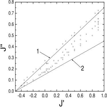
Figure 6: Simulation of spin dynamics at different $J^{\prime}$ and $J^{\prime\prime}$: crosses correspond to a stable Skyrmion, curve 1 corresponds to $J^{\prime\prime}=0.25+0.5\,J^{\prime}$, curve 2 to $J^{\prime\prime}=0.15+0.3\,J^{\prime}$. Simulations are in a good agreement with the criterion of stability against long-wave spin perturbations.

The spin structure of the MBD is shown in Fig. 7. The shape of the bubble is slightly distorted during the collapse. This distortion owes to the effect of the square lattice.

Figure 7: Magnetic bubble generated by numerical simulations. A small square distortion of axial symmetry is caused by symmetry of the lattice. This effect becomes pronounced during the dynamical transformation of the bubble into the Skyrmion. The ratio of the distance between the tip and film is $d/R=7/4$.

We also studied the difference between continuous and discrete approximation by numerical simulations with different anisotropy constants $\lambda$. The discrete models approaches the continuous approximation when anisotropy constant $\lambda$ decreases and the domain wall width $l_{0}$ increases (See Table 1).

Table 1: Normalized parameters of the soliton versus anisotropy constant $\lambda$ derived from numerical simulations. All parameters are normalized to ferromagnetic exchange interaction $J$. Antiferromagnetic exchange interaction constant $J"=0.2$ and $J^{\prime}=0$.

Anisotropy
constant, $\lambda$	0.001	0.0025	0.005	0.01	0.02	0.03	0.04
Effective
AFM	0.19	0.186	0.181	0.175	0.166	0.16	0.155
exchange, $J"_{eff}$
Skyrmion
radius, $R_{s}$	4.28	3.8	3.22	2.77	2.36	2.13	1.97
Domain
wall-width, $l_{0}$	10.39	8.78	7.88	7.36	7.08	6.79	6.53

The process of transformation passes three stages. In the first stage the bubble domain is controlled by the removing tip until it reaches the distance $d\approx 2R$. During the second stage the MBD shrinks under the action of the linear tension. When its radius reaches the value $R\sim l_{0}$, it can not be more described as the MBD and acquires the profile of a Skyrmion. A rough interpolation formula for the transformation time $T(R)$ following from semi-intuitive consideration reads:

$$T\approx{2R\over v}+{R^{2}\over l_{0}\,v_{m}\,\Gamma}+{1\over\omega_{0}\,\Gamma}.$$ (42)

In this equation the first term is the time during which the tip reaches the distance $d=2R$ from the film. At larger distance the interaction between the tip and the film is negligibly small. The second term corresponds to the shrinking of the MBD under the action of the Laplace force from the domain wall. The Laplace force is equal to $F_{L}=\sigma/R$, where $\sigma=2\sqrt{\tilde{J}\lambda}/a$ is the linear tension. The local velocity of the domain wall is antiparallel to the radius and equal to $\eta F_{L}$, where $\eta=\Gamma v_{m}/(4\lambda)$ is the magnetic viscosity. The time $T_{1}(R)$ necessary to decrease significantly the radius is equal to integral

$$T_{1}(R)=\int_{0}^{R}\frac{r\,dr}{\eta\,\sigma}.$$

This gives exactly the second term in equation (42). Finally, the third term is the relaxation time for the Skyrmion derived in Abanov&Pokrovsky98 . This simple interpolation fits the simulation data with very good accuracy.

A more sophisticated description of the transformation process can be obtained by substitution of the interpolation between the MBD and Skyrmion given by equation (29) into the Hamiltonian (1)and integrate it over all variables. The resulting expression is the Hamiltonian for slow variables $R$ and $\psi$. The dimensionless Lagrangian density $l$ can be constructed given the Hamiltonian density $w$ by the following ansatz:

$$l=0.5\,\zeta^{2}\,\frac{\partial\psi}{\partial\tau}-w,$$ (43)

where $\zeta=R_{e}/l_{0}$, $\tau=\omega_{0}t$ and $R_{e}$ is the radius of topological excitation. To incorporate the dissipation it is possible to use the Rayleigh dissipative function $\cal{R}$. In dimensionless variables it reads ${\cal R}=\frac{1}{2}\Gamma\,\zeta\,(\zeta_{\tau}^{2}+\psi_{\tau}^{2}).$ We will not present the equations of motion here to avoid lengthy formulas with no essentially new results. They can be useful when a more detailed description of the process will be in order.

For real magnetic film with $l_{0}\approx 10\,nm$, tip with radius $R=50\,nm$, damping constant $\Gamma=0.1$ and tip’s velocity $v=1\,nm/ns$ transformation time is $T\approx 125\,ns$. The equilibrium size of the Skyrmion is

$$R_{0}=a\left(\,{8J"\over 3\lambda L}\right)^{1/4}\approx 1\div 3\,nm,$$ (44)

where $L=\ln\left[(3\lambda/8J")^{1/4}l_{0}\right]$ and $a$ is the lattice spacing. Skyrmion spin structure obtained by numerical simulations of time-dependent Landau-Lifshitz Equation is represented in Fig. 8.

An effective magnetic field corresponding to the exchange interaction $\tilde{J}$ is $H_{J}=\tilde{J}\,a/\mu_{B}$. For $Fe$ it is about 89 T and for $Co$ it is 112 T. For existing strong magnetic tips real value of created magnetostatic field is about 1 T. Therefore we consider the ratio $H/2\pi\tilde{J}=0.001$. For iron film and tip with radius 50 nm minimum magnetic field of the tip $H_{tip}\approx 28\,G$.

Figure 8: The Stable Skyrmion spin configuration generated from numerical simulations. The anisotropy constant is $\lambda=0.04$, the exchange interaction constants are $J=1$, $J^{\prime}=0.6$, $J"=0.5$.

VIII Conclusions and Discussion

The main result of this work is the numerical evidence that the bubble domain of the 50 nm size initiated by a strong magnetic tip in a thin magnetic film shrinks into a very small, few nanometers metastable Skyrmion. For this purpose we employed the MC and the Runge-Kutta methods on the square lattice. The static Skyrmion and the magnetic bubble domain were found numerically as solutions of the static Landau-Lifshitz equation.

The role of the magnetic tip is two-fold. Its magnetic field stabilizes the bubble domain, which otherwise is unstable in a thin film. Being removed it does not confine the MBD anymore and the latter starts to shrink conserving its topological charge. The Skyrmion is the final result of this shrinking. Thus, the position of the Skyrmion is determined with high accuracy by the tip. This is important for the experimental observation of the Skyrmion, since it is very small and its magnetic field is strongly localized as it was established by our calculations. On the other hand, strong localization of the Skyrmion magnetic field makes possible to read the information stored by Skyrmions if the distances between them and between them and empty spaces are more than $3R_{s}$, where $R_{s}$ is Skyrmion radius. Such a distance is sufficient to ensure that Skyrmions do not perturb the magnetization around.

Limitations on exchange constants accepted in our work stem from the requirement of the Skyrmion stability. One of them is associated with the discrete character of the model and is not essential for a real itinerant magnet with continuous distribution of magnetization. Another one occurs in continuous model: the part of energy proportional to the fourth power of the gradient must be positive. Being imposed onto a lattice model it leads to an inequality, which provides sufficiently large antiferromagnetic exchange between the NNNN. In real itinerant ferromagnets the natural RKKY interaction ensures the stability.

Thus, the Skyrmion stability makes it is possible to create it by circular magnetic tip and to observe it by spin-polarized scanning tunnelling microscopy having a nanometer resolution. It is not yet clear how the creation of the next Skyrmion by lateral scanning tip will influence an already existing Skyrmion. When this problem will be solved, the Skyrmion arrays could be a promising candidate for the magnetic memory of unprecedented high density above 10 TBit/in².

IX acknowledgments

This work has been supported by NSF under the grants DMR0072115 and DMR0103455, by DOE under the grant FG03-96ER45598 and by the Telecommunications and Information Task Force at Texas A&M University.

References

- (1) K. J. Kirk, J. N. Chapman, S. McVite, et al., J. Appl. Phys. 87, 5105 (2000).
- (2) See for example T.H. O’Dell, Ferromagnetodynamics: the dynamics of magnetic bubbles, domains, and domain walls (“A Holsted Press Book”, 1981) and references therein.
- (3) T.H.R. Skyrm, Proc. Roy. Soc. London, A 247, 260 (1958).
- (4) A.A. Belavin and A.M. Polyakov, Pis’ma v ZhETF 22, 503 (1975) [Soviet Physics JETP Letters 22, 245 (1975)] see also A.M. Polyakov, Gauge Fields and Strings (Harwood academic publishers, 1987).
- (5) V.P. Voronov, B.A. Ivanov, and A.K. Kosevich, Zh. Éksp. Teor. Fiz. 84, 2235 (1983)[Spv. Phys. JETP 84, 2235 (1983)].
- (6) B.A. Ivanov, V.A. Stephanovich and A.A. Zhmudskii, J. Magn. Magn. Mater. 88, 116 (1990).
- (7) Ar. Abanov, V.L. Pokrovsky, Phys. Rev. B 58, R8889 (1998).
- (8) F. Kh. Abdullaev, R. M. Galimzyanov and A. S. Kirakosyan, Phys. Rev. B 60, 6552 (1999).
- (9) D. D. Sheka, B. A. Ivanov, and F. G. Mertens, Phys. Rev. B 64, 024432 (2001).
- (10) F.Waldner, J. Magn. Magn. Mater. 31-34, 1203 (1983)
- (11) F.Waldner, J. Magn. Magn. Mater. 54-57, 873 (1986) and Phys. Rev. Lett. 65, 1519 (1990).
- (12) S. L. Sondhi, A. Karlhede, S. A. Kivelson, and E. H. Rezayi, Phys. Rev. B 47, 16419 (1983).
- (13) S.E. Barrett, G. Dabbagh, L.N. Pfeiffer, K. W. West, and R. Tycko, Phys. Rev. Lett. 74, 5112 (1995).
- (14) A. Schmeller, J. P. Eisenstein, L.N. Pfeiffer, and K. W. West, Phys. Rev. Lett. 75, 4290 (1995).
- (15) E.H. Aifer, B.B. Goldberg, and D.A. Broido, Phys. Rev. Lett. 76, 680 (1996).
- (16) M. Schneider, H. Hoffmann, and J. Zweck, Appl. Phys. Lett. 77, 2909 (2000).
- (17) K. Yu. Guslienko and K. L. Metlov, Phys. Rev. B 63, 100403 (2001).
- (18) A. A. Thiele, Bell System Tech. J. 48, 3287 (1969).
- (19) A. A. Thiele, J. Appl. Phys. 41, 1139 (1970).
- (20) H. Callen and R. M. Josephs, J. Appl. Phys. 42, 1977 (1971).
- (21) R. H. Hobart, Proc. Phys. Soc. London 82, 201 (1963)
- (22) G. H. Derrick, J. Math. Phys. 5, 1252 (1964).
- (23) A.M. Kosevich, B.A. Ivanov, and A.S. Kovalev, Phys, Rep. 194, 117 (1990).
- (24) F.D. M. Haldane, Phys. Rev. Lett. 61, 1029 (1988).