Dynamical study on polaron formation in a metal/polymer/metal structure

Abstract

By considering a metal/polymer/metal structure within a tight-binding one-dimensional model, we have investigated the polaron formation in the presence of an electric field. When a sufficient voltage bias is applied to one of the metal electrodes, an electron is injected into the polymer chain, then a self-trapped polaron is formed at a few hundreds of femtoseconds while it moves slowly under a weak electric field (not larger than $1.0\times 10^{4}$ V/cm). At an electric field between $1.0\times 10^{4}$ V/cm and $8.0\times 10^{4}$ V/cm, the polaron is still formed, since the injected electron is bounded between the interface barriers for quite a long time. It is shown that the electric field applied at the polymer chain reduces effectively the potential barrier in the metal/polymer interface.

I introduction

Recent years, organic electronic devices (OEDs), e.g., light-emitting diodes (LEDs) and field-effect transistors (FETs), are attracting considerable interest because they have processing and performance advantages for low-cost and large-area applications.campbell In these devices, organic polymers are used as the light-emitting and charge-transporting layers, in which the electron and/or hole are injected from the metal electrodes and transported under the influence of an external electric field. Due to the strong electron-lattice interactions, it is well known that additional electrons or holes in conjugated polymers will induce self-localized excitations, such as solitonsssh (only in trans-polyacetylene) and polarons.brazovskii As a result, it has been generally accepted that the charge carriers in conjugated polymers are these excitations including both charge and lattice distortion.heeger The formation and transport of such charge carriers are believed to be of fundamental importance for these OEDs.

There have been extensive studies on soliton and polaron dynamics in conjugated polymerssu ; ono ; rakhmanova ; johansson under the influence of external electric fields. It is shown that solitons as well as polarons keep their shape while moving along a chain. Solitons are shown to have a maximum velocity $2.7v_{s}$, where $v_{s}$ is the sound velocity.bishop ; ono The situation will be different for polarons, which has been shown to be not created in electric fields over $6\times 10^{4}$ V/cm due to the charge moving faster and not allowing the distortion to occur.rakhmanova A recent study by Johansson and Stafströmjohansson deals with the polaron migration between neighboring polymer chains. The numerical results show that the polaron becomes totally delocalized, either before or after the chain jump for the electric field over $3\times 10^{5}$ V/cm. There are also studies on the charge transport through metal/polymer interfaces, e.g., the resistance of organic molecular wires attached to metallic surfacesamanta , Schottky energy barriers in metal/organiccampbell2 , and the dynamics of charge transport in a short oligomer sandwiched between two metal contacts.yu

In this paper, we present our results of a non-adiabatic dynamical study on the polaron formation starting from charge injection in a metal/polymer/metal structure in the presence of an external electric field. We would like to focus on charge and its induced lattice distortion in the polymer chain while the metal electrodes at the two ends serves as the source and drain for the extra charges within a tight-binding one-dimensional model. The electron wavefunction is described by the time-dependent Schrödinger equation, in which the transition between instantaneous eigenstates are allowed, while the polymer lattice is treated classically by a Newtonian equation of motion.ono

The paper is organized as follows. In the following section, we present a tight-binding one-dimensional model for the metal/polymer/metal structure and describe the dynamical evolution method. Our results are presented in Sec. III and the summary of this paper is given in Sec. IV.

II model and method

We consider a one-dimensional metal/polymer/metal structure that contains a polymer chain as well as two metal electrodes attached at its two ends. The Hamiltonian consists of three parts,

$$H=H_{e}+H_{latt}+H_{ext}.$$ (1)

The electronic part is

$$H_{e}=-\sum_{n}t_{n}(c_{n}^{\dagger}c_{n+1}+h.c.),$$ (2)

$t_{n}$ being the hopping integral between site $n$ and $n+1$, that is, $t_{n}=t_{0}$ in the two metal electrodes, $t_{n}=t_{0}-\alpha(u_{n+1}-u_{n})$, where $u_{n}$ is the monomer displacement of site $n$ and $\alpha$ describes the electron-lattice coupling between neighboring sites in the polymer chain, as the Su-Schrieffer-Heeger (SSH) modelssh , and $t_{n}=t_{1}$ for the coupling between sites connecting the polymer chain and the metal electrodes. The polymer lattice is described by

$$H_{latt}=\frac{K}{2}\sum_{n}(u_{n+1}-u_{n})^{2}+\frac{M}{2}\sum_{n}\dot{u}_{n}^{2},$$ (3)

where $K$ is the elastic constant and $M$ the mass of a CH group.ssh The contribution from the external field is

$$H_{ext}=\sum_{n}V_{n}(t)(c_{n}^{\dagger}c_{n}-1),$$ (4)

$V_{n}(t)$ being site-energies due to the applied voltage bias and electric field. At the left metal electrode a voltage bias is applied for the charge injection, $V_{n}(t)=V(t)$. At the polymer chain an uniform electric field $E(t)$ is applied, $V_{n}(t)=|e|E(t)[(n-n_{0})a+u_{n}]$ with $e$ being the electron charge, $n_{0}$ the first site of the polymer chain, and $a$ the lattce constant. At the right metal electrode, a field-free area, the site-energies $V_{n}(t)$ are chosen as $V_{n_{1}}(t)$, $n_{1}$ is the last site of the polymer chain. The spin index in the electron operators is omitted since the electron interaction will not be considered here. A similar static model is used very recently to investigate the ground-state properties of ferromagnetic metal/conjugated polymer interfaces.xie

We consider a finite system containing a 200-monomer polymer chain and two 100-site metal electrodes attached at the two ends. The model parameters are those generally chosen for trans-polyacetylene:ssh ; heeger $t_{0}=2.5$eV, $\alpha=4.1$eV$/\AA$, $K=21$eV$/\AA^{2}$, $M=1349.14$eVfs${}^{2}/\AA^{2}$, and $a=1.22\AA$. The coupling between the polymer and the metal is set to $t_{1}=1.0$eV. Before we go further for the dynamical evolution, we determine the static structure of energy levels in a constant external field ($V(t)\equiv V_{0}$ and $E(t)\equiv E_{0}$) in this section.

The total energy is obtained by the expectation value of the Hamiltonian (1) at the half-filled ground state $|g\rangle$,

$$E_{t}=\langle g|H_{e}+H_{ext}|g\rangle+\frac{K}{2}\sum_{n}(u_{n+1}-u_{n})^{2}.$$ (5)

The electronic states are determined by the electronic part of the Hamiltonian (1) and the lattice configuration of the polymer $\{u_{n}\}$ is determined by the minimization of the total energy in the above expression,

$$u_{n+1}-u_{n}=-\frac{\alpha}{K}(\rho_{n,n+1}+\rho_{n+1,n})+\frac{|e|E_{0}}{K}\rho_{n,n}+\lambda,$$ (6)

where $\lambda$ is a Lagrangian multiplier to guarantee the polymer chain length unchanged, i.e., $\sum_{n}(u_{n+1}-u_{n})=0$. $\rho_{n,n^{\prime}}$ is the element of density matrix, which will be given below.

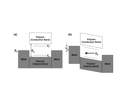
Figure 1: Schematic energy level diagrams of the metal/polymer/metal structure in the absence (a) and presence (b) of external fields. $E_{g}$ is the band gap. The two dashed lines indicate the localized levels if a polaron exists in the polymer chain. $V_{0}$ is the voltage bias applied at the left metal electrode and $E_{0}$ is the electric field applied at the polymer chain.

Due to the coupling between the polymer and the metal electrodes, the electronic states in the polymer and the metal electrodes are mixed. By calculating the wave function possibilities $\eta_{\mu}^{(\kappa)}(\equiv\sum_{n\in\kappa}|\phi_{\mu}(n)|^{2})$ for each state $\mu$, where $\phi_{\mu}(n)$ is the wave function at site $n$ and $\kappa$ is a set of sites (the left metal electrode, the polymer chain, or the right metal electrode) in the system, we can find that each electronic state can be clearly distinguished to be in the polymer or the metal electrodes. It indicates that the coupling $(t_{1}/t_{0})$ in the metal/polymer interfaces is small.

In Fig. 1, we show the schematic energy level diagrams. In the absence of external fields, the polymer chain is dimerized for a half-filled system, the energy band, as in a single polymer chain, has a gap of about $E_{g}=1.32$eV, and the metal electrodes have quasi-continuum bands with the Fermi level almost at the middle of the gap. The dashed lines indicates the localized levels if a polaron exists in the polymer chain. $E_{p}^{\pm}\approx\pm 0.45$eV, indicates the binding energy of a polaron to be about $0.21$eV. It has been known that the energy gap of MEH-PPV is $2.4$eVhag , a much larger value than the energy gap $E_{g}$ we obtained above, but the polaron binding energy is similar to that of MEH-PPV.

In the presence of a constant external field (the voltage bias $V_{0}$ and the electric field $E_{0}$), the energy levels will be changed as shown in Fig. 1(b). The voltage bias $V_{0}$ applied at the left metal electrode raises its energy levels by a value of about $V_{0}$ while the energy levels in other parts are almost unchanged at $E_{0}=0$. It has been shownqiu that when the highest occupied electronic state of the left metal electrode is close to the bottom of the conduction band due to the applied voltage bias ($V_{0}>0.56$eV), the system will be unstable and charges start to be injected into the polymer through the metal/polymer interface. It will be seen that the electric field $E_{0}$ applied at the polymer chain favors the charge injection as a result of the incline of the site-energy at polymer chain.

The voltage bias $V_{0}$ could also serve as the metal work function. At $V_{0}=0$, the energy difference between the electron polaron level in the polymer chain and the highest occupied level of the metal electrode is about 0.45eV. For the contact with MEH-PPV and aluminum, the energy difference is about 1.4eV, and the value is about 0 for that with MEH-PPV and calcium.hag So the value $V_{0}=0.57$eV, we take in the following calculation, could be thought to correspond to that for the Ca/MEH-PPV contact with the voltage bias about 0.2eV applied at the metal calcium.

Now, we describe the non-adiabatic dynamical method that has been used for the dynamics of solitonono and polaronrakhmanova ; johansson in an electron-lattice interacting system. The evolution of the electron wavefunctions depends on the time-dependent Schrödinger equation

$$i\hbar\dot{\phi}_{n,\mu}(t)=-t_{n-1}\phi_{n-1,\mu}(t)+V_{n}(t)\phi_{n,\mu}(t)-t_{n}\phi_{n+1,\mu}(t),$$ (7)

where the site index $n$ runs over the whole chain. The lattice displacements are determined classically by the following Newtonian equations of motion

$$M\ddot{u}_{n}(t) = K[u_{n+1}(t)+u_{n-1}(t)-2u_{n}(t)]$$ (8)

$$+2\alpha[\rho_{n,n+1}(t)-\rho_{n-1,n}(t)]$$

$$+|e|E(t)[\rho_{n,n}(t)-1],$$

where $n$ runs only in the polymer sites. $\rho_{n,n^{\prime}}$ is the element of the density matrix defined as

$$\rho_{n,n^{\prime}}(t)=\sum_{\mu}\phi_{n,\mu}^{*}(t)f_{\mu}\phi_{n^{\prime},\mu}(t),$$ (9)

where $f_{\mu}$ is the time-independent distribution function determined by initial occupation (being 0, 1, or 2). The coupled differential equations (7) and (8) can be solved numerically by use of the same technique in Ref.ono ; johansson . The time step is chosen to be as small as $0.1$fs to avoid numerical errors. A small damping is also introduced to smear out the lattice vibrations, and the effect of the vibrations will be elaborated elsewhere.

In the real calculation, we choose the external field to be turned on smoothly, that is, we let $V(t)=V_{0}\exp[-(t-t_{c})^{2}/t_{w}^{2}]$ for $0<t<t_{c}$ and $V(t)=V_{0}$ for $t\geq t_{c}$ with $t_{c}$ being a smooth turn-on period and $t_{w}$ the width. As the voltage bias $V(t)$, the applied electric field $E(t)$ is also turned on smoothly, i.e., $E(t)=E_{0}\exp[-(t-t_{c})^{2}/t_{w}^{2}]$ for $0<t<t_{c}$ and $E(t)=E_{0}$ for $t\geq t_{c}$ with the same $t_{c}$ and $t_{w}$. In calculations, we take $t_{c}=30fs$, $t_{w}=25fs$, and various values of voltage bias $V_{0}$ and electric field $E_{0}$.

III results

In this section, we present our results on the polaron formation starting from the charge injection from the metal electrode in the presence of an external electric field. For that, we put one extra electron on the lowest unoccupied state of the left metal electrode while the voltage bias and electric field are turned on. In the following, we will focus on the evolution of the charge distribution $\rho_{n}$ [$\equiv\rho_{n,n}-1$] and the staggered lattice configuration $y_{n}$ [$\equiv(-1)^{n}(u_{n}-u_{n-1})$]. At the initial state $(t=0)$, the polymer chain has a dimerized lattice of $y_{n}\approx 0.08\AA$ but a few bonds at its two ends and $\rho_{n}=0$ for all sites in the polymer chain.

First of all, we shows the charge distribution $\rho_{n}$ and the staggered lattice configuration $y_{n}$ (in unit of $\AA$) of the polymer chain at a few typical times under a weak electric field $E_{0}=5\times 10^{3}$V/cm in Fig. 2. The voltage bias applied at the left metal electrode is taken as $V_{0}=0.57$eV, which is just above the minimum value of the bias for the charge injection in the absence of the electric field.qiu For a smaller value of $V_{0}$, the charge will not be injected into the polymer since the energy of the highest occupied electronic level at the left metal electrode ($E_{HO}$) is much lower than the bottom of the conduction band of the polymer ($E_{g}/2$). For a larger value of $V_{0}$, more electrons will be transferred into the polymer since more occupied levels of the left metal electrode will be higher than $E_{g}/2$.

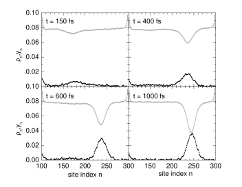
Figure 2: The charge distribution $\rho_{n}$ (solid circles) and the staggered lattice configuration $y_{n}$ (open circles) of the polymer chain at different times under a weak electric field $E_{0}=5\times 10^{3}$V/cm. $V_{0}=0.57$eV.

As the voltage bias applied at the left metal electrode increases to $V_{0}=0.57$eV smoothly, $E_{HO}$ goes up toward the bottom of the conduction band of polymer. At $t=30$fs, $E_{HO}$ reaches its maximum value $0.65$eV, which is very close to the bottom of the conduction band. As a consequence, the coupling between energy levels mainly at the left metal electrode and at the polymer becomes stronger and stronger, the extra electron initially on the left metal electrode begins to be injected into the polymer gradually. From the Fig. 3, which shows the evolution of the total charges in the polymer chain and the metal electrodes, we can see that the charge injection takes a few hundreds of femtoseconds, which seems to be insensitive to the strength of electric fields.

Furthermore, from Fig. 3(a), one can find that the charge does not enter the right metal electrode, which shows the electric field is too weak to overcome the barrier at the right polymer/metal interface, though we have made the calculation up to a few ms. The situation will be different for the electric field $E_{0}>1.0\times 10^{4}$V/cm, see Fig. 3(b), which is strong enough for the charge to overcome the interface barrier and finally enter the right metal electrode in a few thousands fs.

Figure 3: Evolution of the total charges in the polymer chain (line 1) and the metal segments (line 2 and 3) at the electric field $E_{0}=5\times 10^{3}$V/cm (a) and $E_{0}=3.0\times 10^{4}$V/cm (b). $V_{0}=0.57$eV.

In contrast with the case of $E_{0}=0$,qiu the polaron is formed not at the left side of the polymer but at the right side, as shown in Fig. 2, due to the action of the electric field. It will be seen more clearly from Fig. 4, which shows the evolution of the charge center $x_{c}$ in the polymer, which is defined as

$$x_{c}=\sum_{n}n\rho_{n}/\sum_{n}\rho_{n},$$ (10)

where the summation is over the polymer sites. It can be seen that there are two regions, one is the charge injection at $t=0-200$fs, and the other is the polaron formation at $t=200-500$fs. In the first region, the charge is injected into the extended states of the polymer and moves under the electric field. Since the localized lattice distortion has not yet formed in this region, the injected electron behaves as a free conduction electron. As a comparison, we also show the curve for $E_{0}=0$ in Fig. 4, where the charge moves away from the interface just due to the energetic favorite. At a weak electric field, such as $E_{0}=5.0\times 10^{3}$V/cm, the charge center moves gradually to the middle of the polymer chain at $t=200$fs, which corresponds with the charge being almost uniform in the polymer. However, at an electric field with the strength $E_{0}$ between $1.0\times 10^{4}$V/cm and $8.0\times 10^{4}$V/cm, the charge will be spread quickly and then bounced back at the right polymer/metal interface, which is also the reason that the polaron will be formed at a position closer to the left interface under a stronger electric field. In the second region $t=200-500$fs, the lattice distortion makes the polaron form with the charge being trapped inside while it moves toward to the right interface under the electric field.

Figure 4: Evolution of the charge center $x_{c}$ in the polymer chain for various electric fields. $V_{0}=0.57$eV.

What we have found also implies that the polaron will not form in electric fields $\geq 10^{4}$V/cm if the charge does not be bounded by the metal/polymer interfaces. This critical strength of applied electric fields is smaller than that obtained by Rakhmanova and Conwellrakhmanova who gave the value of $6\times 10^{4}$V/cm for the polaron formation but with the initial state of the electron being injected into the polymer chain with the lowest possible energy.

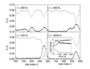
Figure 5: Same as in Fig. 2 but with $E_{0}=1.0\times 10^{5}$V/cm and $V_{0}=0.57$eV. The inset shows the total charges in the polymer chain (solid line) and the metal electrodes (dash and dot-dash lines).

In the case of the electric fields $E_{0}\geq 8.0\times 10^{4}$V/cm, there will be more electrons being injected into the polymer as a result of the incline of the site-energy at polymer chain. In Fig. 5, we show the evolution of the polaron formation for $E_{0}=1.0\times 10^{5}$V/cm. It can be seen from the inset of Fig. 5 that the total charge at the polymer has reached $2e$ at $t=250$fs, when the lattice displays a few distorted wells at random locations. When the charge continues to be injected into the polymer at the period $t=250-1000$fs, the lattice forms a single deep well close to the right interface and the charge also starts to enter the right metal electrode from the polymer under the strong electric field. At around $t=1200$fs, the charge in the polymer decreases to about one electron and a well-shaped polaron locates at the position close to the right interface. It lasts for a few thousands femtoseconds, depending on the strength of the applied field, before the charge enters completely the right metal electrode and the polymer gets back to the dimerized state.

The result for the electric fields $E_{0}\geq 8.0\times 10^{4}$V/cm indicates that the electric field applied at the polymer chain reduces effectively the potential barrier at the metal/polymer interface. To show that, we consider the case of a smaller voltage bias applied at the left metal electrode. For example, we take $V_{0}=0.3$eV, it is found that the charge can be injected into the polymer for the electric fields $\geq 1.7\times 10^{5}$V/cm. In Fig. 6, we show the result of the calculation at the electric field $E_{0}=2.0\times 10^{5}$V/cm and the voltage bias $V_{0}=0.3$eV. The physical process is similar but the polaron lasts only a short period since the charge enters the right metal electrode sooner under a stronger electric field, which also indicates that the potential barrier at the polymer/metal interface is effectively reduced.

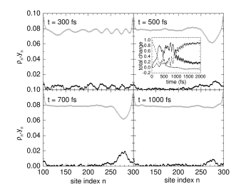
Figure 6: Same as in Fig. 2 but with $E_{0}=2.0\times 10^{5}$V/cm and $V_{0}=0.3$eV. The inset shows the total charges in the polymer chain (solid line) and the metal electrodes (dash and dot-dash lines).

IV summary

In summary, we have investigated the polaron formation starting from the charge injection by using a non-adiabatic dynamic method based on the time-dependent Schrödinger equation for the electronic wavefunctions combining the Newtonian equation of motion for the polymer monomer displacements. It is shown that the polaron is formed while it moves slowly only under a weak electric field $E_{0}<1.0\times 10^{4}$V/cm. But for a stronger electric field, the polaron can be still formed because the charge is not easy to be jumped away from the chain. This result implies that the low mobility of the charge transport in polymers is mainly due to the obstacle for carriers to travel through the polymer/metal interface and/or jump over a neighboring chain. Our results also show that the electric field applied at the polymer chain reduces effectively the potential barrier in the metal/polymer interface.

- (1) I.H. Campbell and D.L. Smith, Solid State Physics, Vol. 55, 1 (2001).
- (2) W.P. Su, J.R. Schrieffer, and A.J. Heeger, Phys. Rev. Lett. 42, 1698 (1979).
- (3) S.A. Brazovskii and N.N. Kirova, Sov. Phys. JETP Lett. 33, 4 (1981).
- (4) A.J. Heeger, S. Kivelson, J.R. Schrieffer, and W.P. Su, Rev. Mod. Phys. 60, 781 (1988).
- (5) W.P. Su and J.R. Schrieffer, Proc. Natl. Acad. Sci. U.S.A. 77, 1839 (1980).
- (6) Y. Ono and A. Terai, J. Phys. Soc. Jpn. 59, 2893 (1990).
- (7) S.V. Rakhmanova and E.M. Conwell, Appl. Phys. Lett. 75, 1518 (1999).
- (8) A. Johansson and S. Stafström, Phys. Rev. Lett. 86, 3602 (2001).
- (9) A.R. Bishop, D.K. Campbell, P.S. Lomdahl, B. Horovitz, and S.R. Phillpot, Phys. Rev. Lett. 52, 671 (1984).
- (10) M.P. Samanta, W. Tian, S. Datta, J.I. Henderson, and C.P. Kubiak, Phys. Rev. B53, R7626 (1996).
- (11) I.H. Campbell, S. Rubin, T.A. Zawodzinski, J.D. Kress, R.L. Martin, D.L. Smith, N.N. Barashkov, and J.P. Ferraris, Phys. Rev. B54, R14321 (1996).
- (12) Z.G. Yu, D.L. Smith, A. Saxena, and A.R. Bishop, Phys. Rev. B59, 16001 (1999).
- (13) S.J. Xie, K.H. Ahn, D.L. Smith, A.R. Bishop, and A. Saxena, Phys. Rev. B67, 125202 (2003).
- (14) I.H. Campbell, T.W. Hagler, D.L. Smith, and J.P. Ferraris, Phys. Rev. Lett. 76, 1900 (1996).
- (15) Y. Qiu, Z. An, and C.Q. Wu, Synth. Met. 135-136, 503 (2003).