Disorder Effect on Spin Excitation in Double Exchange Systems

Abstract

Spin excitation spectrum is studied in the double exchange model in the presence of disorder. Spin wave approximation is applied in the lowest order of $1/S$ expansion. The disorder causes anomalies in the spin excitation spectrum such as broadening, branching, anticrossing with gap opening. The origin of the anomalies is the Friedel oscillation, in which the perfectly polarized electrons form the charge density wave to screen the disorder effect. Near the zone center $q=0$, the linewidth has a $q$ linear component while the excitation energy scales to $q^{2}$, which indicates that the magnon excitation is incoherent. As $q$ increases, there appears a crossover from this incoherent behavior to the marginally coherent one in which both the linewidth and the excitation energy are proportional to $q^{2}$. The results are compared with experimental results in colossal magnetoresistance manganese oxides. Quantitative comparison of the linewidth suggests that spatially-correlated or mesoscopic-scale disorder is more relevant in real compounds than local or atomic-scale disorder. Comparison with other theoretical proposals is also discussed. Experimental tests are proposed for the relevance of disorder.

I Introduction

Since rediscovery of the colossal magnetoresistance (CMR) phenomena, perovskite manganese oxides have attracted much attention. Ramirez1997 ; Coey1999 ; Salamon2001 ; Imada1998 ; Tokura1999 ; Tokura2000 ; Dagotto2001 This family of compounds shows a variety of physical properties in magnetic (ferromagnetism or antiferromagnetism), charge (metal, insulator, or charge ordering), and orbital/lattice (orbital ordering and/or Jahn-Teller distortion) degrees of freedom. Phase transitions between different ordered phases can be controlled by chemical substitution of the A site in the general chemical formula AMnO₃. The magnitude of the CMR effect also changes drastically for different A-site ions, hence, one of the most important issues in this field is to understand the role of the A-site substitution.

The ferromagnetic metallic state, which is widely stable at low temperatures in these compounds, Wollan1955 ; Searle1970 is basically understood by the Zener’s double exchange (DE) mechanism. Zener1951 ; Anderson1955 ; deGennes1960 The kinetics of itinerant electrons in the Mn $e_{g}$ bands strongly correlates with localized spins in the $t_{2g}$ levels through the large Hund’s-rule coupling; ferromagnetism of the localized spins leads to high conductivity of the electrons, and vice versa. Thus, the issue is what is an additional element to the DE interaction which is necessary to explain deviations from this canonical DE behavior and instabilities towards a variety of different phases in the A-site substituted materials.

Among various manganese oxides, it has been recognized that La_1-xSr_xMnO₃ (LSMO) at $x\sim 0.3$ is a canonical DE system. Furukawa1999a Namely, the simple DE model can explain magnetic, transport and optical properties of this material quantitatively. For instance, the experimental value of the Curie temperature $T_{\rm C}$ is well reproduced by recent theoretical calculations in the DE model. Motome2000 ; MotomePREPRINT This material shows relatively high $T_{\rm C}$ compared to other manganese oxides, which also suggests the stability of ferromagnetic metal due to the primary role of the DE mechanism and the irrelevance of other additional factors. This canonical DE system gives a good starting point to examine effects of the A-site substitution.

There are two different ways of the systematic A-site substitution. One is the substitution with different ionic valences, such as the control of $x$ in La_1-xSr_xMnO₃. The mixture of trivalent (La³⁺) and divalent (Sr²⁺) ions effectively changes the nominal valence of manganese ion as Mn^(3+x)+, which controls the electron density in the Mn-O network. The other substitution is by different ionic radii at a fixed valence, such as A_1-xA’_xMnO₃ for different combinations of, for instance, A=La,Pr,Nd,Y and A’=Ba,Sr,Ca at a fixed $x$. These two different substitutions cause systematic and drastic deviations from the canonical DE behavior in LSMO compounds at $x\sim 0.3$.

We discuss mainly the latter A-site substitution with the ionic-radius control in the following. The change of the ionic radii is a sort of the chemical pressure, which modifies length and angle of Mn-O-Mn bonds. This leads to the change of effective transfer integrals between Mn ions, namely, the bandwidth of the electrons. Thus, this substitution has been often called the bandwidth control. This terminology ‘bandwidth control’, however, might be misleading: There are many experimental facts which cannot be explained only by the change of the bandwidth. One is a rapid decrease of $T_{\rm C}$ compared to the bandwidth change. Hwang1995 ; Radaelli1997 $T_{\rm C}$ decreases as the averaged radius of the A ions decreases; however, the change of $T_{\rm C}$ is much larger than that of the bandwidth which is estimated from the structural change. For instance, from La_0.7Sr_0.3MnO₃ to La_0.7Ca_0.3MnO₃ (LCMO), $T_{\rm C}$ decreases by about $30$% while the estimated bandwidth decreases by less than $2$%. Radaelli1997 Since, in the DE theory, $T_{\rm C}$ is proportional to the bandwidth, the large change of $T_{\rm C}$ cannot be explained by the bandwidth change alone. There should be a hidden parameter which strongly suppresses the kinetics of the electrons.

In this work, we focus on the quenched disorder for a candidate of the hidden parameter in this A-site substitution. In general, oxides are known to be far from perfect crystals. Moreover, in these manganese oxides, the disorder is inevitably introduced since they are solid solutions of different A-site ions.

The importance of the disorder has been pointed out in several experimental results: (i) $T_{\rm C}$ changes not only as the average of the ionic radius but also as its standard deviation. Rodriguez-Martinez1996 Even if the average is the same, $T_{\rm C}$ becomes lower for larger standard deviation. (ii) The residual resistivity, namely, the value of the resistivity extrapolated to zero temperature, becomes larger for lower-$T_{\rm C}$ compounds. Coey1995 ; Saitoh1999 (iii) A-site ordered materials, in which different A ions form a periodic ordered structure, exhibit higher $T_{\rm C}$ compared to compounds with random distribution of A ions in the same chemical formula. Millange1998 ; Nakajima2002 ; Akahoshi2003 All these experimental results suggest that the disorder in the random mixture of different size ions scatters the itinerant electrons and suppresses the kinetics of them.

In this paper, we discuss the disorder effect on spin dynamics in the A-site substituted manganites. The spin dynamics is another important indication of a hidden parameter. Spin excitation spectrum shows qualitative changes for the A-site substitution. In compounds with relatively high $T_{\rm C}$ such as LSMO, the spin excitation shows a cosine type dispersion, which is similar to that of Heisenberg spin systems. Perring1996 ; Moudden1998 This behavior is well described by the DE mechanism alone. Furukawa1996 On the contrary, in compounds with low $T_{\rm C}$ such as LCMO, the spectrum shows significant deviations from this form, e.g., some anomalies such as broadening, softening, and gap opening. Hwang1998 ; Vasiliu-Doloc1998 ; Dai2000 ; Biotteau2001 To explain these anomalies is one of the crucial test for elucidating the hidden parameter.

We will demonstrate here that the disorder gives a comprehensive understanding of systematic changes of the spin excitation spectrum as well as other experimental results described above. Several other mechanisms have been proposed, for instance, antiferromagnetic interactions between localized spins, Solovyev1999 orbital degrees of freedom in the $e_{g}$ bands, Khaliullin2000 the electron-lattice coupling, Furukawa1999b and the electron-electron correlation. Kaplan1997 ; Golosov2000 ; Shannon2002 Through the detailed analysis of the spectrum, we will show that the disorder appears to be promising among these scenarios. A part of the results has been published in the previous publications. Motome2002a ; FurukawaPREPRINT ; Motome2003 More systematic and extensive analyses are presented in this paper.

This paper is organized as follows. In Sec. II, we describe methods to study spin dynamics in the DE model. To be self-contained, we derive and summarize some analytical expressions which have been developed in the previous publications. Motome2002a ; FurukawaPREPRINT ; Motome2003 Numerical results are presented in Sec. III for wide regions of parameters. We find remarkable anomalies in the spin excitation spectra and discuss their origin in detail. Comparison with the analytical results is also examined. The results are compared with experimental results as well as with other theoretical ones in Sec. IV. We propose possible experiments to test the relevance of the disorder. Section V is devoted to summary and concluding remarks.

II Formulation

II.1 Model

In this work, we study effects of the disorder on the spin dynamics of the DE model. Zener1951 ; Anderson1955 Our Hamiltonian is given in the form

$${\cal H}= - \sum_{i<j}\sum_{\sigma=\pm}t_{ij}(c_{i\sigma}^{\dagger}c_{j\sigma}+{\rm h.c.})-J_{\rm H}\sum_{i}\mbox{\boldmath$\sigma$}_{i}\cdot\mbox{\boldmath$S$}_{i}$$ (1)

$$+ \sum_{i\sigma}\varepsilon_{i}c_{i\sigma}^{\dagger}c_{i\sigma}.$$

Here, the first term describes the electron hopping between $i$ and $j$th site, the second term represents the Hund’s-rule coupling between the electron spin $\sigma$ (vector of Pauli matrix) and the localized spin $S$, and the last term contains the on-site potential $\varepsilon_{i}$.

In model (1), we take account of the quenched disorder in two ways. One is the off-diagonal disorder in the transfer integral $t_{ij}$ and the other is the diagonal disorder in the potential energy $\varepsilon_{i}$. Hereafter, we call the former the bond disorder and the latter the on-site disorder, respectively. The following discussions in this Sec. II do not depend on the detailed functional form of the distribution of the random variables $t_{ij}$ and $\varepsilon_{i}$. The distribution will be specified in Sec. III.2 for numerical calculations in Sec. III.

II.2 $1/S$ expansion

We apply the spin wave approximation in the lowest order of $1/S$ expansion to model (1) ($S$ is the magnitude of the localized spin $S$). We consider a ferromagnetic ground state with perfect spin polarization $\mbox{\boldmath$S$}_{i}=(0,0,S)$, t_ij and calculate the one-magnon excitation spectrum. In the absence of disorder, the formulation is given in Ref. Furukawa1996, . Here, we extend the method to the case with disorder.

In the presence of disorder, it is convenient to work with the real-space representation instead of the momentum-space one. First, we explicitly diagonalize the Hamiltonian matrix of model (1) for a given configuration of the disorder $\{t_{ij},\varepsilon_{i}\}$. We have

$$\sum_{j}{\cal H}_{ij}(\{t_{ij},\varepsilon_{i}\})\varphi_{n\sigma}(j)=(E_{n}-\sigma J_{\rm H})\varphi_{n\sigma}(i),$$ (2)

where $\varphi_{n\sigma}$ is the $n$th eigenstate with the eigenenergy $E_{n}$. Electron Green’s function is given by

$$G_{ij,\sigma}(\omega)=\sum_{n}\frac{\varphi_{n\sigma}(i)\varphi_{n\sigma}^{*}(j)}{\omega-(E_{n}-\sigma J_{\rm H}-\mu)+{\rm i}\eta\ {\rm sgn}\omega},$$ (3)

where $\mu$ is the chemical potential and $\eta$ is an infinitesimal for convergence. In the lowest order of the $1/S$ expansion, following Ref. Furukawa1996, , the magnon self-energy is obtained from the electron spin polarization function shown in Fig. 1. The contribution from Fig. 1 (a) is given by

$$\Pi_{ii}^{z}(\omega)=\frac{J_{\rm H}}{S}\sum_{n}f_{n+}|\varphi_{n+}(i)|^{2},$$ (4)

where $f_{n+}$ is the fermi distribution function for up-spin states. The other contribution from Fig. 1 (b) is given by

$$\Pi_{ij}^{xy}(\omega)=\frac{2J_{\rm H}^{2}}{S}\sum_{mn}f_{n+}\frac{\varphi_{n+}(i)\varphi_{n+}^{*}(j)\varphi_{m+}(j)\varphi_{m+}^{*}(i)}{\omega+E_{n}-E_{m}-2J_{\rm H}}.$$ (5)

In the limit of $J_{\rm H}\gg t$, which is realistic in CMR manganites, the summation of Eqs. (4) and (5) ends up with

$$\Pi_{ij}(\omega) = \frac{1}{2S}\sum_{mn}f_{n}\varphi_{n}(i)\varphi_{n}^{*}(j)\varphi_{m}(j)\varphi_{m}^{*}(i)$$ (6)

$$\quad\quad\quad\quad\ \ \times(E_{m}-E_{n}-\omega).$$

Here, we assume the orthonormal relation

$$\sum_{m}\varphi_{m}(j)\varphi_{m}(i)=\delta_{ij},$$ (7)

and drop the spin index for simplicity.

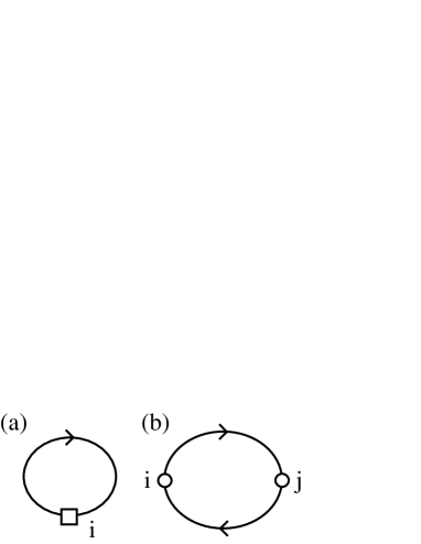
Figure 1: Spin wave self-energy in the lowest order of the $1/S$ expansion. See Ref. Furukawa1996, for details.

Magnon Green’s function is calculated by this self-energy in the form

$$D_{ij}(\omega)=\left[\ \omega-\Pi_{ij}(\omega)+{\rm i}\eta\ \right]^{-1}.$$ (8)

Spin wave excitations are obtained from the poles of the Green’s function (8). Since the self-energy $\Pi_{ij}$ in Eq. (6) is proportional to $1/S$, the positions of the poles are at $\omega\sim O(1/S)$. Hence, within the lowest order of $1/S$ expansion, spin wave excitation is determined by the static part of the self-energy $\Pi_{ij}(\omega=0)$ as discussed in Ref. Furukawa1996, . The matrix inversion in Eq. (8) is easily obtained by using the eigenvectors $\psi_{l}$ and the eigenvalues $\omega_{l}$ which satisfy

$$\sum_{j}\Pi_{ij}(\omega=0)\cdot\psi_{l}(j)=\omega_{l}\psi_{l}(i).$$ (9)

Finally, the spectral function for a given configuration of $\{t_{ij},\varepsilon_{i}\}$ is calculated as

$$A(\mbox{\boldmath$q$},\omega) = -\frac{1}{N}\sum_{ij}\frac{1}{\pi}{\rm Im}D_{ij}(\omega){\rm e}^{{\rm i}\mbox{\boldmath$q$}\cdot(\mbox{\boldmath$r$}_{i}-\mbox{\boldmath$r$}_{j})}$$ (10)

$$= \frac{1}{N}\sum_{l}\Big{|}\sum_{j}\psi_{l}(j){\rm e}^{{\rm i}\mbox{\boldmath$q$}\cdot\mbox{\boldmath$r$}_{j}}\Big{|}^{2}\delta(\omega-\omega_{l}),$$

where $N$ is the system size. The spin excitation spectrum is obtained by averaging $A(\mbox{\boldmath$q$},\omega)$ for random configurations of $\{t_{ij},\varepsilon_{i}\}$. In the same manner, all the physical quantities are to be averaged for random configurations although we do not explicitly remark in the following discussions.

To summarize, the spin excitation spectrum in the DE model is calculated up to the lowest order of the $1/S$ expansion as follows. (i) Diagonalize the Hamiltonian (1) for a configuration of the disorder $\{t_{ij},\varepsilon_{i}\}$, and obtain the electron wavefunction $\varphi_{n}$ and eigenenergy $E_{n}$. (ii) Calculate the magnon self-energy (6) by using $\varphi_{n}$ and $E_{n}$. (iii) Diagonalize the self-energy as in Eq. (9), and obtain the eigenvalues $\omega_{l}$ and eigenvectors $\psi_{l}$. (iv) Calculate $A(\mbox{\boldmath$q$},\omega)$ according to Eq. (10). (v) Repeat (i)-(iv) for different random configurations and take the random average of $A(\mbox{\boldmath$q$},\omega)$.

II.3 Analytical formula

In this section, we derive some analytical expressions for the spin wave excitation. The following framework is general and does not depend on the details of the disorder and the spatial dimension of the system. The derived formulas are useful to discuss the numerical data in the following sections.

II.3.1 Magnon self-energy

First, we examine the static part of the magnon self-energy. We can rewrite $\Pi_{ij}(\omega=0)$ in the form

$$\Pi_{ij}(0)=\frac{1}{2S}\Big{(}{\cal H}_{ij}B_{ji}-\delta_{ij}\sum_{k}{\cal H}_{ik}B_{ki}\Big{)},$$ (11)

where $B_{ij}=\sum_{n}f_{n}\varphi_{n}(j)\varphi_{n}^{*}(i)$. Here, we use the following relations

$$\sum_{m}E_{m}\varphi_{m}(i)\varphi_{m}^{*}(j) = \sum_{mk}{\cal H}_{ik}\varphi_{m}(k)\varphi_{m}^{*}(j)$$ (12)

$$= {\cal H}_{ij},$$

$$\sum_{n}f_{n}E_{n}\varphi_{n}(j)\varphi_{n}^{*}(i) = \sum_{nk}f_{n}{\cal H}_{jk}\varphi_{n}(k)\varphi_{n}^{*}(i)$$ (13)

$$= \sum_{k}{\cal H}_{jk}B_{ki},$$

with the eigenequation (2) and the orthonormality (7).

From Eq. (11), we can easily show that the self-energy satisfies the sum rule in the form

$$\sum_{j}\Pi_{ij}(0)=\frac{1}{2S}\Big{(}\sum_{j}{\cal H}_{ij}B_{ji}-\sum_{k}{\cal H}_{ik}B_{ki}\Big{)}=0.$$ (14)

Thus, the eigenvalue in Eq. (9) always becomes zero at $\mbox{\boldmath$q$}=0$ even in the presence of disorder. This indicates that there is a gapless excitation at $\mbox{\boldmath$q$}=0$. This is consistent with the Goldstone theorem.

We note also that the matrix element of $\Pi_{ij}(0)$ is given by the transfer energy of the electrons. By using the relation

$${\cal H}_{ij}B_{ji}=\sum_{n}f_{n}\varphi_{n}^{*}(i){\cal H}_{ij}\varphi_{n}(j)=\langle{\cal H}_{ij}\rangle,$$ (15)

the matrix elements are written as

$$\Pi_{i\neq j}(0)=-t_{ij}\langle c_{i}^{\dagger}c_{j}\rangle/2S\equiv-2SJ_{ij},$$ (16)

$$\Pi_{ii}(0)=2S\sum_{j}J_{ij},$$ (17)

where we define

$$J_{ij}=t_{ij}\langle c_{i}^{\dagger}c_{j}\rangle/4S^{2}.$$ (18)

The bracket represents the expectation value in the ground state for a given configuration of the disorder. We will show in Sec. II.4 that $J_{ij}$ is the exchange coupling of the corresponding Heisenberg spin model. Equations (16) and (17) indicate that the following summations give the kinetic energy of electrons;

$$\sum_{i\neq j}\Pi_{ij}(0)=-\sum_{i}\Pi_{ii}(0)=\langle{\cal H}_{\rm kin}\rangle/2S,$$ (19)

where ${\cal H}_{\rm kin}$ is the first term in the Hamiltonian (1).

From Eqs. (16) and (17), we note that the magnon self-energy at $\omega=0$ is real in general since $\langle c_{i}^{\dagger}c_{j}\rangle$ is real for the fully-polarized ferromagnetic ground state without degeneracy. Hence, as seen in Eqs. (9) and (10), up to $O(1/S)$, $A(\mbox{\boldmath$q$},\omega)$ for a given configuration of disorder describes a well-defined quasi-particle excitation with infinite lifetime (zero linewidth). Lifetime due to the decay of the quasi particle is obtained from the imaginary part of the poles of Eq. (8), however, it is a higher order term in the $1/S$ expansion. (This higher order correction will be discussed in Sec. IV.2.2.) On the other hand, in the presence of disorder, we have to take the random average for different realizations of disorder configurations. Since different configurations give different $A(\mbox{\boldmath$q$},\omega)$, we obtain a distribution of the excitation spectra after the random average. The distribution gives rise to a finite linewidth, which can be estimated, for instance, by the standard deviation of the excitation energy. This linewidth is due to the so-called inhomogeneous broadening. In the presence of the disorder, this broadening is the lowest order effect in the $1/S$ expansion. We will analyze this linewidth in the following sections.

II.3.2 Spectral function analysis

If the spin excitation spectrum is single-peaked and does not show any splitting, we can apply the following spectral function analysis. We will show in Sec. III that this is the case near the zone center $\mbox{\boldmath$q$}=0$. Let us consider the $m$th moment of the spectral function as

$$\Omega_{\mbox{\boldmath$q$}}^{(m)}=\int_{0}^{\infty}\omega^{m}A(\mbox{\boldmath$q$},\omega)\ d\omega.$$ (20)

Using Eqs. (9) and (10), we obtain

$$\Omega_{\mbox{\boldmath$q$}}^{(m)}=\frac{1}{N}\sum_{ij}\sum_{k_{1}k_{2}...k_{m-1}}\Pi_{ik_{1}}\Pi_{k_{1}k_{2}}\cdot\cdot\cdot\Pi_{k_{m-1}j}{\rm e}^{{\rm i}\mbox{\boldmath$q$}\cdot(\mbox{\boldmath$r$}_{i}-\mbox{\boldmath$r$}_{j})}.$$ (21)

Thus the moment $\Omega_{\mbox{\boldmath$q$}}^{(m)}$ is a Fourier transform of the magnon self-energy $(\Pi_{ij}(0))^{m}$.

The first moment in Eq. (20) gives the averaged excitation energy as

$$\omega_{\rm sw}(\mbox{\boldmath$q$})=\Omega_{\mbox{\boldmath$q$}}^{(1)}.$$ (22)

As mentioned in the last part of Sec. II.3.1, the linewidth is estimated by the standard deviation of the excitation energy which is given by the second moment in the form

$$\gamma(\mbox{\boldmath$q$})=\big{[}\ \Omega_{\mbox{\boldmath$q$}}^{(2)}-(\Omega_{\mbox{\boldmath$q$}}^{(1)})^{2}\ \big{]}^{1/2}.$$ (23)

II.3.3 Excitation energy

Here, we analyze the excitation energy of Eq. (22). Substituting Eqs. (20) and (21) into Eq. (22), we obtain

$$\omega_{\rm sw}(\mbox{\boldmath$q$})=\frac{1}{N}\sum_{ij}\Pi_{ij}{\rm e}^{{\rm i}\mbox{\boldmath$q$}\cdot(\mbox{\boldmath$r$}_{i}-\mbox{\boldmath$r$}_{j})}.$$ (24)

When model (1) has the electron hopping only between the nearest neighbor sites, the magnon self-energy $\Pi_{ij}$ has nonzero matrix elements only for $i=j$ and $i=j+\mbox{\boldmath$\eta$}$ as shown by Eqs. (16) and (17). Here $\eta$ is a displacement vector to the nearest neighbor site. Then the excitation energy is given as

$$\omega_{\rm sw}(\mbox{\boldmath$q$}) = \frac{1}{N}\sum_{i}\Big{(}\Pi_{ii}+\sum_{\mbox{\boldmath$\eta$}}\Pi_{i,i+\mbox{\boldmath$\eta$}}\ {\rm e}^{{\rm i}\mbox{\boldmath$q$}\cdot\mbox{\boldmath$\eta$}}\Big{)}$$ (25)

$$= \sum_{\mbox{\boldmath$\eta$}}\ \bar{\Pi}(\mbox{\boldmath$\eta$})\ ({\rm e}^{{\rm i}\mbox{\boldmath$q$}\cdot\mbox{\boldmath$\eta$}}-1),$$

where we define the site-averaged quantity $\bar{\Pi}(\mbox{\boldmath$\eta$})=\sum_{i}\Pi_{i,i+\mbox{\boldmath$\eta$}}/N$ and use the sum rule Eq. (14). Even in the presence of the disorder, the symmetry for the direction of $\eta$ is expected to be recovered after the random average, therefore we assume

$$\bar{\Pi}(\mbox{\boldmath$\eta$})=\frac{1}{z}\sum_{\mbox{\boldmath$\eta$}}\bar{\Pi}(\mbox{\boldmath$\eta$})\equiv-\Lambda,$$ (26)

where $z$ is the number of coordinates. Finally, we obtain the following form

$$\omega_{\rm sw}(\mbox{\boldmath$q$})=\Lambda\sum_{\mbox{\boldmath$\eta$}}(1-{\rm e}^{{\rm i}\mbox{\boldmath$q$}\cdot\mbox{\boldmath$\eta$}}).$$ (27)

This indicates that on hypercubic lattices the excitation spectrum shows the cosine dispersion even in the presence of disorder. In the limit of $q=|\mbox{\boldmath$q$}|\rightarrow 0$, we have

$$\omega_{\rm sw}(\mbox{\boldmath$q$})\simeq\Lambda q^{2}.$$ (28)

Thus, the quantity $\Lambda$ gives the spin wave stiffness. In our analysis, the stiffness is proportional to the kinetic energy of electrons as

$$\Lambda=-\frac{1}{z}\sum_{\mbox{\boldmath$\eta$}}\bar{\Pi}(\mbox{\boldmath$\eta$})=-\frac{1}{zN}\sum_{i\mbox{\boldmath$\eta$}}\Pi_{i,i+\mbox{\boldmath$\eta$}}=-\frac{\langle{\cal H}_{\rm kin}\rangle}{2SzN},$$ (29)

where we use Eq. (19).

II.3.4 Linewidth

Next, we analyze the linewidth of Eq. (23). Similarly to the derivation of Eq. (25), the second moment of the spectral function is written in the form

$$\Omega_{\mbox{\boldmath$q$}}^{(2)}=\sum_{\mbox{\boldmath$\eta$}_{1}\mbox{\boldmath$\eta$}_{2}}\ \bar{\Pi}_{2}(\mbox{\boldmath$\eta$}_{1},\mbox{\boldmath$\eta$}_{2})(1-{\rm e}^{{\rm i}\mbox{\boldmath$q$}\cdot\mbox{\boldmath$\eta$}_{1}})(1-{\rm e}^{{\rm i}\mbox{\boldmath$q$}\cdot\mbox{\boldmath$\eta$}_{2}}),$$ (30)

where

$$\bar{\Pi}_{2}(\mbox{\boldmath$\eta$}_{1},\mbox{\boldmath$\eta$}_{2})=\frac{1}{N}\sum_{i}\Pi_{i+\mbox{\boldmath$\eta$}_{1},i}\Pi_{i,i+\mbox{\boldmath$\eta$}_{2}},$$ (31)

and $\mbox{\boldmath$\eta$}_{1}$ and $\mbox{\boldmath$\eta$}_{2}$ are the displacement vectors to the nearest neighbor site. In the absence of disorder, we have $\Pi_{i+\mbox{\boldmath$\eta$},i}=\Pi_{i,i+\mbox{\boldmath$\eta$}}=-\Lambda$. Hence, the linewidth $\gamma$ becomes zero since $\Omega_{\mbox{\boldmath$q$}}^{(2)}=(\Omega_{\mbox{\boldmath$q$}}^{(1)})^{2}$. In the presence of disorder, the linewidth becomes finite. For simplicity, we consider here the linewidth in a special direction such as $\mbox{\boldmath$q$}=(q,0,0,\cdot\cdot\cdot)$ on a hypercubic lattice. Since $\bar{\Pi}_{2}$ in Eq. (31) generally depends on the relative direction between $\mbox{\boldmath$\eta$}_{1}$ and $\mbox{\boldmath$\eta$}_{2}$, we represent two different cases as

$$\bar{\Pi}_{2}(\mbox{\boldmath$\eta$}_{1},\mbox{\boldmath$\eta$}_{2})=\Lambda_{2}\pm\delta\Lambda_{2}\quad\mbox{for \ $\mbox{\boldmath$\eta$}_{1}=\pm\mbox{\boldmath$\eta$}_{2}$}.$$ (32)

Then, Eq. (30) is rewritten as

$$\Omega_{\mbox{\boldmath$q$}}^{(2)}=4\big{(}\ \Lambda_{2}(1-\cos q)^{2}+\delta\Lambda_{2}\sin^{2}q\ \big{)}.$$ (33)

In the limit of $q\rightarrow 0$, we have

$$\gamma^{2}(\mbox{\boldmath$q$})\simeq c_{1}q^{2}+c_{2}q^{4},$$ (34)

where

$$c_{1} = 4\ \delta\Lambda_{2},$$ (35)

$$c_{2} = \Lambda_{2}-\frac{4}{3}\ \delta\Lambda_{2}-\Lambda^{2}.$$ (36)

Therefore, in the presence of disorder, the linewidth shows a $q$ linear behavior in the small $q$ regime.

II.3.5 Incoherence of spin wave excitation

From the above analysis, we obtain $\omega_{\rm sw}\propto q^{2}$ and $\gamma\propto q$ in the limit of $q\rightarrow 0$ as in Eqs. (28) and (34). Thus, the linewidth $\gamma$ becomes larger than the excitation energy $\omega_{\rm sw}$ at $\mbox{\boldmath$q$}\sim 0$, which indicates that the spin wave excitation becomes incoherent or localized.

This incoherent behavior comes from local fluctuations. The $q$ linear coefficient in $\gamma$ in Eq. (35) is given by the difference of $\bar{\Pi}_{2}$ for different directions of $\eta$, which is proportional to

$$c_{1} \propto \bar{\Pi}_{2}(\mbox{\boldmath$\eta$},\mbox{\boldmath$\eta$})-\bar{\Pi}_{2}(\mbox{\boldmath$\eta$},-\mbox{\boldmath$\eta$})$$ (37)

$$\propto \sum_{i}(\Pi_{i+\mbox{\boldmath$\eta$},i}-\Pi_{i,i-\mbox{\boldmath$\eta$}})^{2}$$

$$\propto \sum_{i}(J_{i+\mbox{\boldmath$\eta$},i}-J_{i,i-\mbox{\boldmath$\eta$}})^{2},$$

where we use Eq. (16). From the definition of $J_{ij}$ in Eq. (18), Eq. (37) shows that the $q$ linear coefficient $c_{1}$ is proportional to the local fluctuations of the transfer energy of electrons.

As $q$ becomes large, we have a crossover from this incoherent regime where $\gamma\propto\omega_{\rm sw}^{1/2}\propto q$ to the marginally coherent regime where $\gamma\propto\omega_{\rm sw}\propto q^{2}$. This crossover is determined by the coefficients $c_{1}$ and $c_{2}$ in Eqs. (35) and (36). These coefficients depend on the details of parameters in the system, especially on the type of the disorder, as will be discussed in Sec III.5.2.

II.4 Correspondence to Heisenberg model

Here, we discuss the relation between the spin excitation spectra in the DE model (1) and those in the Heisenberg spin model whose Hamiltonian is given by ${\cal H}_{\rm Heis}=-2\sum_{i<j}J_{ij}\mbox{\boldmath$S$}_{i}\cdot\mbox{\boldmath$S$}_{j}$. As explicitly shown in Appendix A, the static part of the magnon self-energy (11) corresponds to the effective spin-wave Hamiltonian for the Heisenberg model within the leading order of the $1/S$ expansion. There, Eq. (18) gives the relation between the kinetics of itinerant electrons in the DE model (1) and the exchange coupling $J_{ij}$ in the Heisenberg model. This relation provides us physical intuitions to understand our results.

In the absence of disorder, when we consider the transfer $t_{ij}=t$ only for the nearest neighbor sites, $J_{ij}$ in Eq. (18) becomes a constant $J$ which is nonzero only for $i=j+\mbox{\boldmath$\eta$}$. Thus, as noted in Ref. Furukawa1996, , the spin excitation spectrum in the pure DE model with infinite $J_{\rm H}$ is equivalent to that in the Heisenberg model with the nearest neighbor exchange $J_{ij}=J$, and is given by the simple cosine dispersion.

Disorder introduces some randomness in the expectation value of $\langle c_{i}^{\dagger}c_{j}\rangle$ as well as the transfer integral $t_{ij}$. This leads to the nonuniform exchange coupling $J_{ij}$ in the corresponding Heisenberg model. It is instructive to compare the spectrum for the DE model and that for the Heisenberg model with random exchange couplings $J_{ij}$ which no longer satisfy the relation (18). (See also Sec. III.4.3.) For the random Heisenberg model, the spin wave stiffness $\Lambda$ is given by the random average of the exchange constant $J_{ij}$. Moreover, the $q$ linear term in the linewidth is determined by local fluctuations of the random exchange $J_{ij}$. Thus, these aspects are commonly observed both in the random DE model and in the random Heisenberg model even if the relation (18) does not hold between them. In other words, in the long wavelength limit of $q\rightarrow 0$, the magnetic excitation has a similar structure between these two models, although one is the itinerant electron system and the other is the localized spin system. However, for moderate or large $q$, the excitation spectrum of the DE model in the presence of disorder shows remarkable differences from that of the random Heisenberg model as shown in Sec. III. There, the fermionic properties of itinerant electrons play a key role through the expectation value $\langle c_{i}^{\dagger}c_{j}\rangle$.

III Results

III.1 Overview

In this section, we show numerical results which are obtained based on the method described in Sec. II.2. After the specification of the functional form of the disorder distribution in Sec. III.2, we show that the spin excitation spectrum exhibits some anomalies due to the disorder in Sec. III.3. We examine the anomalies in detail by changing parameters such as strength and type of the disorder, spatial dimensions, and doping concentration. We discuss the origin of these anomalies in Sec. III.4. In Sec. III.5, we examine quantitative aspects of the excitation spectrum by applying the spectral function analysis in Sec. II.3.2 to the numerical results. We compare them with the analytical expressions obtained in Sec. II.3.

III.2 Distribution form of disorder

In the following sections, we consider the on-site disorder $\varepsilon_{i}=\delta\varepsilon$ and the bond disorder $t_{ij}=t+\delta t$ only for the nearest neighbor sites where $\delta\varepsilon$ and $\delta t$ obey one of the following three distribution functions. The first one is the binary distribution in the form

$$P(x)=\frac{1}{2}\big{[}\ \delta(\Delta)+\delta(-\Delta)\ \big{]},$$ (38)

namely, $x=+\Delta$ or $-\Delta$ in the equal probability. The second one is the Gaussian distribution in the form

$$P(x)=\frac{1}{\sqrt{2\pi}\Delta}\exp\Big{(}-\frac{x^{2}}{2\Delta^{2}}\Big{)}.$$ (39)

The last one is the box distribution in the form

$$P(x)=\frac{1}{2p}\Theta(x+p)\big{(}1-\Theta(x-p)\big{)},$$ (40)

where $p=\sqrt{3}\Delta$ and $\Theta(x)$ is the Heaviside step function. The normalizations are taken to give the same second moment as $\int x^{2}P(x)dx=\Delta^{2}$.

In the following calculations, we consider the hypercubic lattice in $d$ dimensions, and we take the half-bandwidth $W=zt=2dt$ for $J_{\rm H}=\Delta=0$ as an energy unit. We change the value of $\Delta$ as a parameter typically up to $0.5W$. It is difficult to determine the realistic value of $\Delta$ in low $T_{\rm C}$ manganites. A rough estimate has been given by the first principle calculation, which shows that $\Delta$ becomes the same order of magnitude of the half-bandwidth $W$. Pickett1997

III.3 Anomaly in spin excitation spectrum

III.3.1 Dependence on strength and type of disorder

We first show the change of the spin excitation spectrum by controlling the strength of the disorder in Fig. 2. Here, we fix the doping concentration at $x=0.3$, where the hole density $x$ is defined as $x=1-\langle\sum_{i}c_{i}^{\dagger}c_{i}/N\rangle$ (we drop the spin index because the ground state is perfectly polarized). Numerical calculations are performed for $N=20\times 20\times 20$ site clusters under the periodic boundary conditions. The results are for the on-site disorder whose distribution is given by the binary form of Eq. (38). The spectrum is obtained by the random average of $A(\mbox{\boldmath$q$},\omega)$ in Eq. (10) over $16$ different realizations of random configurations for each value of $\Delta$. The gray-scale contrast shows the intensity of the spectrum.

Figure 2: Spin excitation spectra at $x=0.3$ in the presence of the on-site disorder in the binary distribution with (a) $\Delta=0$, (b) $\Delta=0.1$, (c) $\Delta=0.2$, and (d) $\Delta=0.3$, respectively.

In the case of $\Delta=0$, i.e., in the absence of the disorder, the spin excitation spectrum is given by a cosine dispersion as shown in Fig. 2 (a). When we switch on the disorder, the excitation shows a finite linewidth which becomes large as $\Delta$ increases. Moreover, as clearly seen in Figs. 2 (c) and (d), the spectrum shows some anomalies in the large $q$ region. There, we have additional broadening as well as branching, that is, an emergence of an additional branch which has significantly lower energy than the original cosine like excitation. For large values of $\Delta$, the lower branch has a substantial weight as shown in Fig. 2 (d). If one follows only the lower branch, the spectrum appears to show softening near the zone boundary.

These anomalous features are commonly observed irrespective of the type of the disorder. Figure 3 shows the results for different distribution functions; (a) is for the Gaussian distribution of Eq. (39) and (b) is for the box distribution of Eq. (40). In both cases, we have similar anomalous features to those in Fig. 2.

Figure 3: Spin excitation spectra at $x=0.3$ in the presence of the on-site disorder with $\Delta=0.3$ in (a) the Gaussian distribution and (b) the box distribution.

We also examine the case of the bond disorder in Fig. 4. Here, we consider the binary distribution (38) for $\delta t$. In this case also, the spectrum shows additional broadening which is more prominent and makes a branching obscure compared to the cases of the on-site disorder in Figs. 2 and 3. This is related to strong incoherence in the case of the bond disorder which will be discussed quantitatively in Sec. III.5.

Figure 4: Spin excitation spectrum at $x=0.3$ in the presence of the bond disorder in the binary distribution with $\Delta=0.15$.

III.3.2 Spatial dimension dependence

Next, we examine systems in less spatial dimensions, namely, in two and one dimensions. In manganites, there are compounds which have strong two-dimensional anisotropy, such as the bilayer materials A₃Mn₂O₇ and the single-layer materials A₂MnO₄. Later, we will discuss the quantitative comparison between our results and experimental ones in these compounds in Sec. IV. Here, we calculate $40\times 40$ site clusters for $50$ different realizations of random configurations in the two-dimensional (2D) case, and $256$ site clusters for $500$ configurations in the one-dimensional (1D) case.

Figure 5: Spin excitation spectra in (a) two dimensions and (b) one dimension. The results are for $x=0.3$ with the on-site disorder in the binary distribution with $\Delta=0.3$.

Figure 5 shows the excitation spectra in 2D and 1D systems at $x=0.3$ for the on-site disorder in the binary distribution of Eq. (38) with $\Delta=0.3$. In both dimensions, the spectra show the anomalies clearly as in three-dimensional (3D) systems in Sec. III.3.1. The important aspect is that in lower dimensions the anomalous features appear more apparently. Especially, in the 1D case in Fig. 5 (b), the detailed structure of the anomalies can be observed. There, we have anticrossing with gap opening and shadow-band like features. From this systematic study for different dimensions, we speculate that the branching observed in higher dimensions is a remnant of this anticrossing.

The anticrossing with the gap opening reminds us of the electron dispersion in systems with spin density wave or collective phonon mode. In these systems, magnons or phonons scatter the electrons and open a gap with the anticrossing in the dispersion. This analogy will be discussed further in Sec. III.4.1.

III.3.3 Doping dependence

Here, we study the doping dependence in a systematic way. Figure 6 shows the results for different hole concentrations $x$ in 3D cases. We consider here the on-site disorder whose distribution is given by the binary form of Eq. (38) with $\Delta=0.2$. Figure 6 shows that the anomalous features become apparent as $x$ decreases. This is probably because the disorder strength becomes relatively large compared to the kinetic energy of electrons which becomes small as $x$ decreases. Moreover, we note that the positions of the anomalies appear to shift as $x$.

Figure 6: Spin excitation spectra in three dimensions for (a) $x=0.5$, (b) $x=0.4$, (c) $x=0.3$, and (d) $x=0.2$, respectively. The results are for the on-site disorder in the binary distribution with $\Delta=0.2$.

In order to observe the $x$ dependence more clearly, we study the 1D systems under the same conditions. Figure 7 shows the results. As indicated in the figures, the position of the anomalous features clearly shift as the change of $x$, and is around the Fermi wavenumber $k_{\rm F}$ which is given by $\pi(1-x)$ in this 1D case ($k_{\rm F}$ is for the spinless fermion in the perfectly polarized ground state). We note also that the relatively weak anomalies can be observed additionally at $q\sim\pi-k_{\rm F},2k_{\rm F},2(\pi-k_{\rm F})$, and so on. These indicate that the anomalies are closely related to the fermionic degrees of freedom. This observation provides a key to understand the origin of the anomalies.

Figure 7: Spin excitation spectra in one dimension for (a) $x=0.5$, (b) $x=0.4$, (c) $x=0.3$, and (d) $x=0.2$, respectively. The results are for the on-site disorder in the binary distribution with $\Delta=0.2$. The dashed lines represent the Fermi wavenumber at each $x$.

III.4 Origin of the anomaly

III.4.1 Friedel oscillation

We summarize the aspects of the anomalies of the spin excitation spectrum which are observed in the previous section. (i) There appear additional broadening, branching, anticrossing with gap opening, and shadow band. (ii) These anomalous features are observed universally for different types of the disorder, spatial dimensions and doping concentrations. (iii) The anomalies become more apparent in lower dimensions. (iv) They appear most conspicuously at $\mbox{\boldmath$q$}\sim\mbox{\boldmath$k$}_{\rm F}$ while the additional anomalies can be seen at $\mbox{\boldmath$q$}\sim\mbox{\boldmath$Q$}-\mbox{\boldmath$k$}_{\rm F},2\mbox{\boldmath$k$}_{\rm F},2(\mbox{\boldmath$Q$}-\mbox{\boldmath$k$}_{\rm F})$, etc where $\mbox{\boldmath$Q$}=(\pi,\pi,\cdot\cdot\cdot)$.

As mentioned in Sec. III.3.2, the anticrossing structure suggests a scattering mechanism for magnons. Moreover, as shown in Sec. III.3.3, this scattering is characterized by the Fermi wavenumber $\mbox{\boldmath$k$}_{\rm F}$, which suggests that the scatterers are closely related with the fermionic degrees of freedom. From these points, we consider that the origin of the anomalies is the Friedel oscillation. Friedel1953

The mechanism is as follows. In the presence of disorder, electrons tend to screen the effects of disorder, which leads to the charge density correlation with the wavenumber $2\mbox{\boldmath$k$}_{\rm F}$. This is the so-called Friedel oscillation. Friedel1953 In this DE system, the charge density wave is equivalent to the spin density wave since the ground state is the fully polarized ferromagnetic state (half-metallic state Park1998 ). Thus, we have the $2\mbox{\boldmath$k$}_{\rm F}$ spin density correlation due to the disorder though it is nonmagnetic. The spin density oscillation couples to magnon excitations and scatters them. This leads to the anticrossing features near $\mbox{\boldmath$q$}=\mbox{\boldmath$k$}_{\rm F}$. (Note that the scattering wavenumber $2\mbox{\boldmath$k$}_{\rm F}$ corresponds to the scattering between $\mbox{\boldmath$q$}\sim\mbox{\boldmath$k$}_{\rm F}$ and $-\mbox{\boldmath$k$}_{\rm F}$.) The Friedel oscillation itself is a general phenomenon in fermionic systems with disorder, and its effect becomes relatively weaker in higher dimensions. These aspects are consistent with our observations mentioned above. Therefore, we conclude that the Friedel oscillation is the origin of the spin excitation anomalies in this system.

III.4.2 Single impurity problem

In order to confirm the picture based on the Friedel oscillation, we examine the problem with a single impurity. In this case, the charge density correlation is clearly found around the impurity position. Figure 8 (a) shows the density distribution in the real space when we introduce a single impurity in the 1D system with $N=256$. Here, $n_{i}=\langle c_{i}^{\dagger}c_{i}\rangle$ and we put the on-site potential at $i=128$ with relatively large $\varepsilon_{i}=-5$ to enlarge the impurity effect in the spectrum. The electron density oscillates around the impurity site, which results in the singularity at $q=2k_{\rm F}$ in the density correlation function as shown in Fig. 8 (b). Note that $q=0.6\pi$ corresponds to $2k_{\rm F}$ with the hole Fermi wavenumber $k_{\rm F}=0.3\pi$ (or $2\pi-2k_{\rm F}$ with the electron Fermi wavenumber $k_{\rm F}=0.7\pi$). Here, we define the density correlation function as

$$N(q)=\frac{1}{N}\sum_{ij}n_{i}n_{j}\ {\rm e}^{{\rm i}q(i-j)}.$$ (41)

In this case of the single impurity also, as shown in Fig. 8 (c), the spin excitation spectrum shows weak but obvious anomalies at $k=k_{\rm F},\pi-k_{\rm F}$, etc., which are similar to the results in the previous section III.3. The position of the anomalies is solely determined by $k_{\rm F}$ while their strength depends on the number and the strength of the disorder. This strongly supports our scenario of the Friedel oscillation.

Figure 8: (a) Local electron density when the on-site potential is finite only at the site $i=128$. (b) Density correlation function. (c) Spin excitation spectrum. The dashed line in (c) represents the Fermi wavenumber.

III.4.3 Comparison with random exchange Heisenberg model

In Sec. II.4, we discussed the correspondence between the DE model and the Heisenberg spin model within the spin wave approximation. There, Eq. (18) gives a relation between these two models, where the exchange coupling $J_{ij}$ is given by the expectation value $\langle c_{i}^{\dagger}c_{j}\rangle$. In order to show the fermionic effect in this quantity explicitly, we study here the spin excitation in the Heisenberg model with completely random exchange couplings. Namely, we consider the ferromagnetic Heisenberg model with the nearest-neighbor exchange couplings $J_{ij}^{({\rm r})}$ which take random values from bond to bond and no longer satisfy Eq. (18). This will elucidate a contrast from the random DE model (1). Within the lowest order of $1/S$ expansion, this model leads to the effective spin-wave Hamiltonian in the form

$${\cal H}_{i\neq j}=-2SJ_{ij}^{({\rm r})},\quad\ {\cal H}_{ii}=2S\sum_{j}J_{ij}^{({\rm r})}.$$ (42)

(See Appendix A.) Although this effective Hamiltonian has a similar structure to the magnon self-energy and satisfies the sum rule Eq. (14), it is nothing to do with the fermionic degrees of freedom in the DE model. We calculate the spin excitation from Eqs. (42) in 1D. A typical spectrum is shown in Fig. 9. Here, we choose $J_{ij}^{({\rm r})}$ randomly from the range of $1-\Delta\leq J_{ij}^{({\rm r})}\leq 1+\Delta$ with $\Delta=0.25$. We find no notable anomalies except for the broadening for the entire spectrum in contrast to the results in Sec. III.3. This result supports the above picture and elucidates the relevance of the fermionic degrees of freedom of itinerant electrons to the spin excitation in the random DE model.

Figure 9: Spin excitation spectrum in the Heisenberg spin model with random exchange couplings. See the text for details.

III.5 Quantitative aspects of the spectrum

As shown in Sec. III.3, although the spin excitation spectrum exhibits significant anomalies near the Fermi wavenumber $\mbox{\boldmath$k$}_{\rm F}$, it appears to be always single-peaked near the zone center $\mbox{\boldmath$q$}=0$. This allows us to apply the spectral function analysis in Sec. II.3.2 in this regime. In this section, we discuss the quantitative aspects of the excitation spectrum by applying the spectral function analysis to the numerical results in comparison with the analytical expressions obtained in Secs. II.3.3 and II.3.4. Throughout this section, we consider the binary distribution (38) for both cases of the bond disorder and the on-site disorder.

III.5.1 Spin wave stiffness and magnon bandwidth

As shown in Eq. (29), the stiffness $\Lambda$ is proportional to the kinetic energy of electrons per site in our analysis. Figure 10 plots the stiffness as a function of $\Delta$ at $x=0.3$, which is calculated from the magnon self-energy by using Eq. (26). In all dimensions, the stiffness decreases as the disorder becomes strong. The asymptotic dependence in the limit of $\Delta\rightarrow 0$ appears to be $\Lambda\propto\Delta^{2}$.

Figure 10: Spin stiffness at $x=0.3$ as a function of $\Delta$. Circles, squares, and triangles represent the results in one, two, and three dimensions, respectively. Open and filled symbols correspond to the cases of the bond disorder and the on-site disorder, respectively. The lines are guides for the eye.

Next we consider the bandwidth of the spin excitation. In the pure system without disorder, the total bandwidth of the spin wave excitation $E_{\rm sw}$ is determined by the spin stiffness $\Lambda$ in the form $E_{\rm sw}=2z\Lambda$. Furukawa1996 Thus, from Eq. (26), the spin wave bandwidth $E_{\rm sw}$ is proportional to the kinetic energy of electrons per site in the absence of disorder. This relation no longer holds in the presence of disorder. We estimate the bandwidth $E_{\rm sw}$ by the peak energy of the highest excitation at $\mbox{\boldmath$q$}=(\pi,\pi,\pi)$ in 3D systems. Figure 11 plots the estimates of $E_{\rm sw}$ as a function of the strength of the on-site disorder $\Delta$. Although the stiffness always decreases as the disorder strength increases, the change of the bandwidth $E_{\rm sw}$ depends on the hole concentration $x$: $E_{\rm sw}$ decreases for $x\mathrel{\mathchoice{\lower 2.5pt\vbox{\halign{$\m@th\displaystyle\hfil#\hfil$\cr>\crcr\sim\crcr}}}{\lower 2.5pt\vbox{\halign{$\m@th\textstyle\hfil#\hfil$\cr>\crcr\sim\crcr}}}{\lower 2.5pt\vbox{\halign{$\m@th\scriptstyle\hfil#\hfil$\cr>\crcr\sim\crcr}}}{\lower 2.5pt\vbox{\halign{$\m@th\scriptscriptstyle\hfil#\hfil$\cr>\crcr\sim\crcr}}}}0.3$, however, $E_{\rm sw}$ increases for $x\mathrel{\mathchoice{\lower 2.5pt\vbox{\halign{$\m@th\displaystyle\hfil#\hfil$\cr<\crcr\sim\crcr}}}{\lower 2.5pt\vbox{\halign{$\m@th\textstyle\hfil#\hfil$\cr<\crcr\sim\crcr}}}{\lower 2.5pt\vbox{\halign{$\m@th\scriptstyle\hfil#\hfil$\cr<\crcr\sim\crcr}}}{\lower 2.5pt\vbox{\halign{$\m@th\scriptscriptstyle\hfil#\hfil$\cr<\crcr\sim\crcr}}}}0.3$. At $x\sim 0.3$, $E_{\rm sw}$ remains almost constant in this range of $\Delta$. This indicates that in our DE system at $x\sim 0.3$, although the spectrum near the zone center becomes narrower due to the decrease of the stiffness as the disorder becomes stronger, the total bandwidth of the spin excitation is almost unchanged. Indeed, this behavior is observed in Fig. 2.

Figure 11: Total bandwidth of the spin excitation spectrum in three dimension with the on-site disorder. Circles, squares, and crosses represent the results for $x=0.4,0.3$, and $0.2$, respectively. The lines are guides for the eye.

III.5.2 Excitation energy and linewidth

The spectral function analysis in Sec. II.3.2 concludes the excitation energy $\omega_{\rm sw}\propto q^{2}$ and the linewidth $\gamma\propto q$ in the limit of $q\rightarrow 0$. Figure 12 shows the small $q$ behaviors of $\omega_{\rm sw}$ and $\gamma$ which are calculated from the numerical data by using Eqs. (22) and (23). All the numerical results in different dimensions show consistent $q$ dependences with the analytical predictions. We also confirm that there is the incoherent regime where $\gamma>\omega_{\rm sw}$ near $\mbox{\boldmath$q$}=0$. These justify the applicability of the spectral function analysis which is based on the assumption of the single-peaked structure of the spectrum.

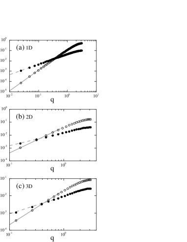
Figure 12: $q$ dependence of the excitation energy (open circles) and the linewidth (filled circles) at $x=0.3$ in the presence of the on-site disorder in the binary distribution $\Delta=0.2$ in (a) one, (b) two, and (c) three dimensions, respectively, along $\mbox{\boldmath$q$}=(q,0,0,\cdot\cdot\cdot)$. The gray solid (dashed) lines are the fits to $q^{2}$ ($q$).

Figure 13 plots the values of the coefficient of the $q$ linear term, $c_{1}$ in Eq. (34) as a function of the stiffness $\Lambda$ by changing the disorder strength $\Delta$. As $\Lambda$ decreases ($\Delta$ increases), $c_{1}$ increases almost linearly to the decrease of $\Lambda$. The interesting point is that the coefficient $c_{1}$ increases much faster in the case of the bond disorder than the on-site disorder. This indicates that the bond disorder induces larger $q$ linear term, namely, stronger incoherence in the magnon excitation than the on-site disorder.

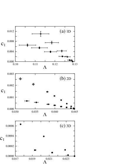
Figure 13: $q$ linear coefficient $c_{1}$ in the linewidth as a function of the spin stiffness in (a) one, (b) two, and (c) three dimensions, respectively. Open and filled symbols correspond to the cases of the bond disorder and the on-site disorder, respectively.

This point is clearly demonstrated when we plot the linewidth as a function of the excitation energy as shown in Figs. 14 and 15. For the bond disorder (Fig. 14), the behavior $\gamma\propto\omega_{\rm sw}^{1/2}$ dominates the spectrum. On the contrary, for the on-site disorder (Fig. 15), the $\omega_{\rm sw}^{1/2}$ part is observed only in the small $q$ regime, and the behavior $\gamma\propto\omega_{\rm sw}$ is dominant in the wide region of $q$. There, we have a crossover from the incoherent behavior with $\gamma\propto\omega_{\rm sw}^{1/2}\propto q$ to the marginally coherent behavior with $\gamma\propto\omega_{\rm sw}\propto q^{2}$. Qualitative features are universal irrespective of the spatial dimensions.

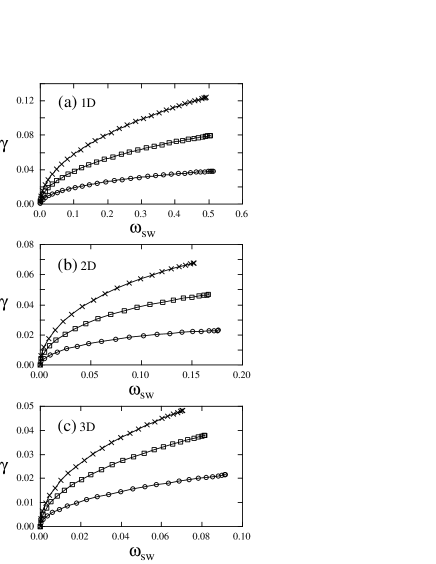
Figure 14: Linewidth as a function of excitation energy in the case of the bond disorder. The results are for $x=0.3$ in (a) one, (b) two, and (c) three dimensions, respectively, along $\mbox{\boldmath$q$}=(q,0,0,\cdot\cdot\cdot)$. Circles, squares, and crosses represent $\Delta=0.05,0.1$, and $0.15$, respectively.

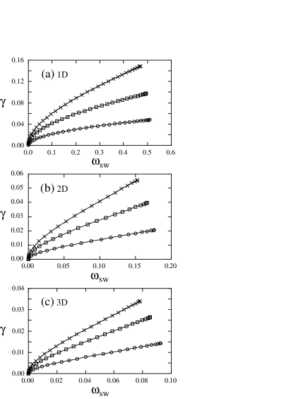
Figure 15: Linewidth as a function of excitation energy in the case of the on-site disorder. The results are for $x=0.3$ in (a) one, (b) two, and (c) three dimensions, respectively, along $\mbox{\boldmath$q$}=(q,0,0,\cdot\cdot\cdot)$. Circles, squares, and crosses represent $\Delta=0.1,0.2$, and $0.3$, respectively.

We find here the qualitatively different behavior between the bond disorder and the on-site disorder in the crossover from the incoherent to the marginally coherent regime. Considering this difference and its origin, we will discuss a general tendency of this crossover and a realistic type of the disorder in real compounds in Sec. IV.3.

IV Discussions

IV.1 Spin excitation anomalies in low-$T_{\rm C}$ manganites

In high-$T_{\rm C}$ manganites, such as La_1-xSr_xMnO₃ and La_1-xPb_xMnO₃ near $x=0.3$, the spin excitation spectrum shows a cosine like dispersion, Perring1996 ; Moudden1998 which can be well explained by the pure DE model without disorder (Fig. 2 (a)). Furukawa1996 Contrast to this canonical DE behavior, low-$T_{\rm C}$ manganites such as Pr_1-xSr_xMnO₃, La_1-xCa_xMnO₃, and Nd_1-xSr_xMnO₃ show the following anomalous features in the spin excitation spectrum.

One of the remarkable anomalies is called the softening. Hwang et al. reported a significant softening of the spin wave dispersion near the zone boundary in Pr_1-xSr_xMnO₃ at $x=0.37$. Hwang1998 Later, Dai et al. confirmed this result in several materials, and observed the optical phonon mode in the energy range where the softening occurs. Dai2000 A similar spectrum with the optical phonon branch has been obtained also in the bilayer manganite, La_2-2xSr_1+2xMn₂O₇ at $x=0.4$. Furukawa2000 In this compound, however, a qualitatively different spectrum, which is a cosine like form without any softening, has been observed in the same chemical formula but in a different sample crystal. Perring2001 This suggests the strong sample dependence of this softening behavior.

Another anomaly is the broadening. Hwang1998 ; Vasiliu-Doloc1998 ; Dai2000 In compounds which show the softening, the linewidth of the excitation becomes significantly large in the region where the softening is observed. An important aspect is that the linewidth remains finite even at the lowest temperature where the ferromagnetic moment is fully saturated. This point will be discussed in Sec. IV.2.2.

In compounds with relatively small $x$ (low doping), the spin excitation shows another anomaly such as the gap opening and/or the anticrossing. Vasiliu-Doloc1998 ; Biotteau2001 Note that the ground state in these compounds is ferromagnetic insulator and not metal. The phase diagram in the small $x$ region shows complicated transitions in structural and magnetic degrees of freedom accompanied by a dimensional crossover. Wollan1955 ; deGennes1960 ; Kawano1996a ; Kawano1996b

As shown in the results in Sec. III, our simple model (1), i.e., the DE model with disorder, reproduces all the above anomalies, at least, in a quantitative level. The softening appears in the lower energy branch in the anticrossing. The additional broadening is observed in the large $q$ regime. These anomalies become more conspicuous in lower doped case and in lower dimensions. These agreements suggest that the disorder is a candidate to give a reasonable description on the large spectral changes from the high-$T_{\rm C}$ to the low-$T_{\rm C}$ manganites. However, besides our disorder scenario, there have been many other theoretical proposals for the present problem. We compare our results with those by other scenarios in the following.

IV.2 Comparison with other theoretical results

IV.2.1 Softening

Several mechanisms have been proposed for the softening near the zone boundary. One is the purely magnetic origin, i.e., due to competitions between the DE ferromagnetic and the superexchange antiferromagnetic interactions between localized spins including longer ranged couplings. Solovyev1999 Other scenarios take account of a coupling to other degrees of freedom. One proposal is the coupling to orbital fluctuations, in which orbital degrees of freedom in the doubly degenerate $e_{g}$ orbitals are explicitly taken into account. Khaliullin2000 Another proposal is the coupling to phonons which leads to the anticrossing between the phonon excitation and the magnon excitation. Furukawa1999b

Although all these scenarios including our disorder scenario can reproduce the lower ‘softened’ energy excitation in experimental results, there are some qualitative differences. In our results, the softening does not occur in the strict sense, because the lower energy excitation appears just as a result of the anticrossing. We still have the higher energy branch near the original dispersion in the absence of the disorder. If one follows only the lower branch, it looks like the softening as pointed out in Sec. III.3.1. On the contrary, the mechanisms of the magnetic origin and of the magnon-orbital coupling origin cause the softening of the original dispersion itself, hence there is no higher energy branch. In the scenario of the magnon-phonon coupling, the spectrum shows a similar structure to our anticrossing. However, in this case, the lower excitation near the zone boundary is originally the optical phonon mode, which extends over the whole Brillouin zone with almost flat dispersion (optical mode). There should be a finite energy excitation even at the zone center additionally to the gapless magnon excitation. This is different from our results in which the spectrum is single-peaked near the zone center. These qualitative differences can be distinguished experimentally by studying the high energy excitation in the wide region of the Brillouin zone. This kind of experimental tests will be discussed and summarized in Sec. IV.4.

Besides the above qualitative differences, our disorder scenario is different from the other proposals quantitatively. In other scenarios, it should be noted that the relative importance of the additional couplings is determined by the change of the DE interaction, namely, the bandwidth, since the strength of them does not change so much by the A-site substitution. In this sense, these scenarios attribute the origin of the change of the spectrum from high-$T_{\rm C}$ to low-$T_{\rm C}$ compounds to the change of the bandwidth. As discussed previously, however, the actual change of the bandwidth in these compounds is very small. Therefore, it appears to be difficult for these scenarios to explain the large changes of the spin excitations in a quantitative manner. On the contrary, the strength of the disorder can be largely affected by the A-site substitution even if the change of the averaged lattice structure is small. This appears to favor our disorder scenario.

IV.2.2 Broadening

As discussed in Sec. IV.1, the experimental results show the intrinsic linewidth at the lowest temperature. This suggests that the spin wave excitation is no longer the eigenstate of the system at the ground state. We discuss here two different mechanisms for this zero-temperature broadening. One is effective even in the absence of disorder and the other is our disorder scenario.

Even in the pure DE model without disorder, the spin wave is not the exact eigenstate of the system. Kaplan1997 The coupling with charge degrees of freedom leads to a finite lifetime for the spin wave excitations. This zero-temperature broadening in the pure DE model has been discussed by the spin wave approximation. Golosov2000 ; Shannon2002 In the lowest order of the $1/S$ expansion, the DE model can be mapped to the pure Heisenberg model as discussed in Appendix A. Hence, the spin wave is the exact eigenstate and the linewidth is zero in $O(1/S)$. Furukawa1996 In the higher order of $1/S$, however, we have a finite imaginary part in the magnon self-energy, which leads to a linewidth in the spin excitation spectrum. Up to $O(1/S^{2})$, this linewidth is predicted to show the $q$ dependence as $\gamma\propto q^{d+3}$ in the limit of $q\rightarrow 0$, where $d$ is the spatial dimension of the system. Thus, the linewidth is predicted to behave as $\gamma\propto q^{6}$ in 3D and $\gamma\propto q^{5}$ in 2D systems.

In the presence of disorder, our results indicate that the spin excitation spectrum shows a finite linewidth even in the lowest order of $1/S$ expansion. As discussed in Sec. II.3.1, this is an inhomogeneous broadening and distinguished from the above broadening due to the finite lifetime of quasiparticle excitations. In our results, the linewidth shows the $q$ linear behavior in the limit of $q\rightarrow 0$, and crossovers to the $q^{2}$ behavior as $q$ increases. These behaviors do not depend on the spatial dimension $d$. Therefore, it is possible to determine which scenario is relevant in real compounds by studying the $q$ dependence of the linewidth in both 3D and 2D systems.

In 2D (bilayer) compounds, recently, detailed analyses have been done on the $q$ dependence of the linewidth. Perring2001 The marginally coherent behavior $\gamma\propto\omega_{\rm sw}\propto q^{2}$ is observed in the wide region of $q$. It is difficult to explain this $q$ dependence by the former mechanism which predicts $\gamma\propto q^{5}$ in 2D. In our disorder scenario, the marginally coherent behavior is actually found as shown in Sec. III.5.2. This supports our scenario.

Unfortunately, the linewidth in the small $q$ region has not been fully investigated experimentally, especially in 3D compounds in the ferromagnetic metallic regime. Hwang1998 ; Dai2000 Detailed information near the zone center especially for $q\mathrel{\mathchoice{\lower 2.5pt\vbox{\halign{$\m@th\displaystyle\hfil#\hfil$\cr<\crcr\sim\crcr}}}{\lower 2.5pt\vbox{\halign{$\m@th\textstyle\hfil#\hfil$\cr<\crcr\sim\crcr}}}{\lower 2.5pt\vbox{\halign{$\m@th\scriptstyle\hfil#\hfil$\cr<\crcr\sim\crcr}}}{\lower 2.5pt\vbox{\halign{$\m@th\scriptscriptstyle\hfil#\hfil$\cr<\crcr\sim\crcr}}}}\pi/5$ is lacking. Further experimental study is desired to examine the asymptotic $q$ dependence.

In our results, the crossover between the incoherent regime and the marginally coherent regime appears to depend on the details of the disorder as mentioned in Sec. III.5.2. The dominance of the marginally coherent behavior in experimental results provides us a microscopic picture on the disorder in real compounds. This will be discussed in Sec. IV.3 in detail.

IV.2.3 Anticrossing and gap opening

As mentioned in Sec. IV.1, the gap opening and/or the anticrossing have been experimentally observed only in the low doped region ($x\mathrel{\mathchoice{\lower 2.5pt\vbox{\halign{$\m@th\displaystyle\hfil#\hfil$\cr<\crcr\sim\crcr}}}{\lower 2.5pt\vbox{\halign{$\m@th\textstyle\hfil#\hfil$\cr<\crcr\sim\crcr}}}{\lower 2.5pt\vbox{\halign{$\m@th\scriptstyle\hfil#\hfil$\cr<\crcr\sim\crcr}}}{\lower 2.5pt\vbox{\halign{$\m@th\scriptscriptstyle\hfil#\hfil$\cr<\crcr\sim\crcr}}}}0.2$) where $T_{\rm C}$ is largely reduced from the value at $x\simeq 0.3$. Vasiliu-Doloc1998 ; Biotteau2001 In this region, the kinetic energy becomes small partly because the number of carriers decreases. There, the system is insulating with ferromagnetism or spin canting as well as the orthorhombic lattice distortion. Wollan1955 ; deGennes1960 ; Kawano1996a ; Kawano1996b Hence, there should be competitions among several interactions such as ferromagnetic DE, antiferromagnetic superexchange, and electron-lattice interaction.

We note that, in the 3D system, the values of $\Delta$ in the present calculations are much smaller than the critical value for the Anderson localization, Li1997 ; Sheng1997 hence, the ground state remains the ferromagnetic metal in our results. In lower dimensions, of course, electrons are easily localized at small $\Delta$. The ferromagnetic or the spin canting state indicates the relevance of the DE interaction even in the insulating states. The charge/spin oscillation due to the disorder is expected even in these insulators although the Fermi wavenumber is no longer well defined. Hence, we expect similar anomalies in these insulating regions.

Besides our disorder scenario, we have at least two mechanisms which cause the anticrossing and/or the gap opening in the spin excitation spectrum. One is the superlattice magnetic structure such as the spin canting. In this case, the spin excitation spectrum shows a gap at the wavenumber for the corresponding magnetic periodicity. The spectrum consists of a single branch in the extended Brillouin zone and deviates from the cosine like form only near the gap. The small gap observed at $\mbox{\boldmath$q$}=(0,0,\pi/2)$ in La_0.85Sr_0.15MnO₃ appears to be explained by this scenario since the corresponding superlattice peak is observed. Vasiliu-Doloc1998 This behavior should be distinguished from the anticrossing or the branching in our results.

The other mechanism is the magnon-phonon coupling as mentioned in Sec. IV.2.1. Furukawa1999b In this scenario, the anticrossing with the gap opening appears at the wavenumber where the magnon dispersion crosses the optical phonon branch. The excitation spectrum looks similar to our results. Possible experimental tests to distinguish these scenarios will be discussed in Sec. IV.4.

IV.3 Atomic vs. mesoscopic scale disorder

Our results in Sec. III.5.2 elucidate a difference in the spin excitation between the bond disorder and the on-site disorder. In the case of the on-site disorder, the crossover from the incoherent behavior $\gamma\propto\omega_{\rm sw}^{1/2}\propto q$ to the marginally coherent one $\gamma\propto\omega_{\rm sw}\propto q^{2}$ takes place in the relatively small $q$ region, and the latter behavior is dominant in the wide region of the spectrum. On the other hand, in the case of the bond disorder, the incoherent behavior dominates over the whole $q$ region. The bond disorder tends to make the spectrum more incoherent than the on-site disorder in the present model.

Since the incoherence comes from the local fluctuations of $J_{ij}$ in Eq. (18) as discussed in Sec. II.3.5, this difference indicates that the bond disorder leads to relatively larger fluctuations of $J_{ij}$ than the on-site disorder in the present model. This is qualitatively understood as follows. In Eq. (18), there are two sources of the local fluctuations of $J_{ij}$. One is the transfer integral $t_{ij}$ and the other is the expectation value $\langle c_{i}^{\dagger}c_{j}\rangle$. In the case of the on-site disorder, $t_{ij}$ is taken to be uniform for all the nearest neighbor pairs, hence, the local fluctuations come only from $\langle c_{i}^{\dagger}c_{j}\rangle$. This expectation value is disordered in the presence of disorder, however, it has some correlations due to the Friedel oscillation as discussed in Sec. III.4. On the contrary, in the case of the bond disorder, $t_{ij}$ is taken to be completely independent from bond to bond in our model. This local fluctuation of $t_{ij}$ is directly reflected in that of $J_{ij}$ in Eq. (18). Even if there are some spatial correlations in $\langle c_{i}^{\dagger}c_{j}\rangle$, the multiplication of $t_{ij}$ makes $J_{ij}$ more disordered. Thus, in the present model, we expect a larger local fluctuations in the case of the bond disorder than the on-site disorder.

However, this does not mean that the bond disorder always makes the spin excitation spectrum more incoherent than the on-site disorder in general. The stronger incoherence in the present results is due to the specific form of $t_{ij}$ in our model. Even in the case of the bond disorder, the incoherence is possibly suppressed if we have some spatial correlations in $t_{ij}$. Instead, the important conclusion is that the atomic-scale disorder leads to more incoherent excitation than the spatially-correlated or the mesoscopic-scale disorder.

As discussed in Sec. IV.2.2, the experimental results in the bilayer compounds show the dominance of the marginally coherent regime. From the above conclusion, this indicates that in real materials the mesoscopic-scale disorder is more relevant than the atomic-scale disorder if the disorder plays a major role in the spin excitation spectrum. Possible sources of the mesoscopic-scale disorder are a large-scale inhomogeneity or clustering of the A ions, twin lattice structure, and grain boundaries.

IV.4 Experimental tests

We propose here some experiments to test our disorder scenario.

(i) Sample dependence: Our scenario predicts a correlation between the sample quality and the anomalies in the spin excitation spectrum. Even in the same chemical formula, the extent of the anomalies may depend on the sample quality. The purity of samples can be measured independently, for instance, by the magnitude of the residual resistivity. In this test, we note that the A-site ordered manganites Millange1998 ; Nakajima2002 ; Akahoshi2003 will be useful. In these materials, the disorder strength due to the alloying effect in the A-site ions can be tuned to some extent by the careful treatment of the syntheses. It is interesting to compare the spin excitation spectrum in the A-site ordered compound with that in the ordinary solid-solution (A-site disordered) compound in the same chemical formula.

(ii) Comparison with the Fermi surface: The spin excitation anomalies in our results appear strongly near the Fermi wavenumber. It is crucial to compare the position of the anomalies with the information of the Fermi surface. The Fermi surface can be independently determined, for instance, by the angle-resolved photoemission spectroscopy.

(iii) Doping dependence: Closely related to the above test (ii), the doping dependence is also a key experiment. In our scenario, by controlling the doping concentration, the position of the anomalies shifts due to the change of the Fermi surface. Moreover, the anomalies become more conspicuous for lower doping concentration.

(iv) High energy excitation: Our scenario predicts the anticrossing instead of the softening. Hence, near the zone boundary, there remains the higher energy excitation above the lower energy branch which looks like to be softened. As discussed in Sec. IV.2.1, this point is different from several other theoretical proposals. At the same time, it is important to identify the optical phonon mode, especially near the zone center, for examining the relevance of the magnon-phonon coupling as discussed in Sec. IV.2.1. Therefore, it is crucial to study the higher energy region over the whole Brillouin zone.

(v) $q$ dependence of the linewidth: Our results indicate that irrespective of the spatial dimension, the linewidth of the spectrum is proportional to $q$ near the zone center and shows a crossover to $q^{2}$ behavior as $q$ increases. As discussed in Sec. III.5.2, this $q$ dependence appears to be consistent with the experimental result in the bilayer manganite. In all other scenarios, the linewidth in the ground state comes from the interplay between charge and spin which is discussed in Sec. IV.2.2. This predicts $q^{d+3}$ behavior near the zone center. It is strongly desired to examine the linewidth more quantitatively especially in 3D compounds.

V Summary and concluding remarks

In this paper, we have discussed the disorder effects on the spin excitation spectrum in the double exchange model. We have applied the spin wave approximation in the lowest order of $1/S$ expansion. The analytical expressions are obtained for the spin stiffness, the excitation energy, and the linewidth. The most important result revealed by the extensive numerical calculations is that the spin excitation spectrum shows some anomalies in the presence of the disorder, such as broadening, branching, or anticrossing with gap opening. The origin of these anomalies is the Friedel oscillation: Disorder causes the $2k_{\rm F}$ oscillation of the spin and charge density in the fully polarized ferromagnetic state, which scatters the magnons to cause the anticrossing in their dispersion. Thus, the spin excitation anomalies are the consequence of the strong interplay between spin and charge degrees of freedom. Our results have been compared with experimental results in the A-site substituted manganites which shows relatively low-$T_{\rm C}$, and the agreement is satisfactory. We have also compared our results with other theoretical proposals for the anomalous spin excitation in these manganites, and clarified the advantages of our disorder scenario.

Another important finding is the incoherence of the magnon excitation. We have shown that near the zone center the linewidth is proportional to the magnitude of the wavenumber $q$, which becomes larger than the excitation energy which scales to $q^{2}$. This incoherence comes from the local fluctuations of the transfer energy of itinerant electrons. As $q$ increases, we have obtained the crossover from this incoherent behavior to the marginally coherent one in which both the linewidth and the excitation energy are proportional to $q^{2}$. We found that this crossover behavior depends on the nature of the disorder. Comparing with experimental results in which the marginally coherent behavior is dominant, we have concluded that in real materials the spatially-correlated or mesoscopic-scale disorder is relevant compared to the local or atomic-scale disorder.

All the above anomalous features are obtained in the lowest order of the $1/S$ expansion, $O(1/S)$. Up to $O(1/S)$, we have shown that the double exchange model with disorder is effectively mapped to the Heisenberg spin model with random exchange couplings. In the absence of the disorder, the corresponding Heisenberg model has the uniform nearest neighbor exchanges, whose spin excitation spectrum shows the cosine dispersion. Furukawa1996 ; FurukawaPREPRINT Even in this pure case, in the higher order of $1/S$, there are some deviations from this cosine dispersion such as the magnon bandwidth narrowing or the softening, and the broadening. Kaplan1997 ; Golosov2000 ; Shannon2002 However, these higher order corrections are known to be small near the hole concentration $x=0.3$ where we are interested in. Kaplan1997 Moreover, the spin excitation anomalies we obtained here are the primary effects in the $1/S$ expansion compared to the higher-order corrections. Therefore, we believe that our results are relevant to understand the anomalous spin excitations in real compounds. Our results give a comprehensive understanding of the systematic changes of the spin excitation spectrum in the A-site substituted manganites. Moreover, the disorder explains well the experimental facts which cannot be understood only by the bandwidth control, such as the rapid decrease of $T_{\rm C}$. MotomePREPRINT Therefore, we conclude that the disorder plays an important role in the A-site substitution of the ionic radius control in CMR manganites.

We comment on the relevance of another additional couplings due to the influence of the multicritical phenomena. As decreasing the ionic size of the A-site atoms, finally the system becomes the charge-ordered insulator with the orbital and lattice orderings, the ferromagnetic insulator, the antiferromagnetic insulator, or the spin glass insulator. Imada1998 ; Hwang1995 ; Goodenough1955 ; DeTeresa1997 ; Tomioka2002 The phase diagram often shows the multicritical behavior. These phase transitions might not be explained by the disorder alone. In the close vicinity of the multicritical phase boundary, we expect large fluctuations and critical enhancement of additional couplings, which possibly accelerate the suppression of $T_{\rm C}$ and enhance the anomalies in the spin excitation spectrum. However, the multicritical phenomena is essentially the first order phase transition. Hence, far from the phase boundary, for instance, in LCMO compounds, we believe that these additional couplings becomes irrelevant and the disorder plays a major role.

Appendix A

In this Appendix, we show that the magnon self-energy (11) is equivalent to the effective spin-wave Hamiltonian for the Heisenberg spin model in the lowest order of the $1/S$ expansion. FurukawaPREPRINT

We begin with model (1) in the limit of $J_{\rm H}/t\rightarrow\infty$. In this limit, since the conduction electron spin $\sigma$ is completely parallel to the localized spin at each site, states with $\sigma$ antiparallel to $S$ are projected out. Then, we have the effective spinless-fermion model as Anderson1955

$${\cal H}=-\sum_{ij}(\tilde{t}_{ij}c_{i}^{\dagger}c_{j}+{\rm h.c.})+\sum_{i}\varepsilon_{i}c_{i}^{\dagger}c_{i},$$ (43)

where the transfer integral $\tilde{t}_{ij}$ depends on the relative angle of localized spins as

$$\tilde{t}_{ij}=t_{ij}\Big{[}\cos\frac{\theta_{i}}{2}\cos\frac{\theta_{j}}{2}+\sin\frac{\theta_{i}}{2}\sin\frac{\theta_{j}}{2}{\rm e}^{-{\rm i}(\phi_{i}-\phi_{j})}\Big{]},$$ (44)

with $S_{i}^{x}=S\sin\theta_{i}\cos\phi_{i}$, $S_{i}^{y}=S\sin\theta_{i}\sin\theta_{i}$, and $S_{i}^{z}=S\cos\theta_{i}$. Hereafter, we treat the localized spins $S$ as classical objects. The transfer integral in Eq. (43) is a complex variable. The real and imaginary parts are given by

$${\rm Re}\ \tilde{t}_{ij} = t_{ij}\sqrt{\frac{1}{2}\Big{(}1+\frac{\mbox{\boldmath$S$}_{i}\cdot\mbox{\boldmath$S$}_{j}}{S^{2}}\Big{)}},$$ (45)

$${\rm Im}\ \tilde{t}_{ij} = \frac{t_{ij}}{2}\sqrt{\frac{S^{2}}{(S+S_{i}^{z})(S+S_{j}^{z})}}\frac{S_{i}^{y}S_{j}^{x}-S_{i}^{x}S_{j}^{y}}{S^{2}},$$ (46)

respectively. Note that ${\rm Im}\ \tilde{t}_{ij}$ is antisymmetric while ${\rm Re}\ \tilde{t}_{ij}$ is symmetric, as expected from $\tilde{t}_{ij}=\tilde{t}_{ji}^{*}$.

Now we apply the spin wave approximation to model (43). We use here the Holstein-Primakoff transformation

$$S_{i}^{z} = S-a_{i}^{\dagger}a_{i},$$

$$S_{i}^{x} \simeq \sqrt{\frac{S}{2}}(a_{i}^{\dagger}+a_{i}),\ \ S_{i}^{y}\simeq{\rm i}\sqrt{\frac{S}{2}}(a_{i}^{\dagger}-a_{i}),\$$ (47)

and take account of the $1/S$ expansion up to the leading order of $O(1/S)$. Substituting Eqs. (47) into Eqs. (45) and (46), we obtain

$$\frac{{\rm Re}\ \tilde{t}_{ij}}{t_{ij}} \simeq 1+\frac{1}{4S}(a_{i}^{\dagger}a_{j}+a_{j}^{\dagger}a_{i}-a_{i}^{\dagger}a_{i}-a_{j}^{\dagger}a_{j}),$$ (48)

$$\frac{{\rm Im}\ \tilde{t}_{ij}}{t_{ij}} \simeq \frac{1}{4S}(a_{i}^{\dagger}a_{j}-a_{j}^{\dagger}a_{i}).$$ (49)

Hence, the effective magnon-electron Hamiltonian up to $O(1/S)$ is given by

$${\cal H} \simeq -\sum_{ij}t_{ij}\Big{[}1+\frac{1}{4S}(a_{i}^{\dagger}a_{j}+a_{j}^{\dagger}a_{i}-a_{i}^{\dagger}a_{i}-a_{j}^{\dagger}a_{j})\Big{]}$$ (50)

$$\quad\quad\quad\quad\quad\times(c_{i}^{\dagger}c_{j}+c_{j}^{\dagger}c_{i})$$

$$+\frac{1}{4S}\sum_{ij}t_{ij}(a_{i}^{\dagger}a_{j}-a_{j}^{\dagger}a_{i})(c_{i}^{\dagger}c_{j}-c_{j}^{\dagger}c_{i})$$

$$+\sum_{i}\varepsilon_{i}c_{i}^{\dagger}c_{i}.$$

Finally, we obtain the effective magnon Hamiltonian by tracing out the fermion degrees of freedom in Eq. (50). Up to $O(1/S)$, the trace can be calculated as the expectation value for the ground state without any magnon. The result is given by

$${\cal H}\simeq-\sum_{ij}\frac{t_{ij}}{2S}\langle c_{i}^{\dagger}c_{j}\rangle(a_{i}^{\dagger}a_{j}+a_{j}^{\dagger}a_{i}-a_{i}^{\dagger}a_{i}-a_{j}^{\dagger}a_{j}),$$ (51)

up to irrelevant constants. Here we use the general relation $\langle c_{i}^{\dagger}c_{j}\rangle=\langle c_{j}^{\dagger}c_{i}\rangle$ for the perfectly polarized ground state without degeneracy. Note that this effective Hamiltonian is derived generally for both the bond disorder and the on-site disorder. From the eigenvalues and the eigenvectors for Eq. (51), we obtain the spectral function $A(\mbox{\boldmath$q$},\omega)$. Hence, comparing with Eqs. (9) and (10), the static part of the magnon self-energy $\Pi(\omega=0)$ is equivalent to the effective magnon Hamiltonian (51).

This effective Hamiltonian (51) has the same form as that for the Heisenberg spin model ${\cal H}_{\rm Heis}=-2\sum_{i<j}J_{ij}\mbox{\boldmath$S$}_{i}\cdot\mbox{\boldmath$S$}_{j}$ within the leading order of the $1/S$ expansion. This correspondence gives the relation between the kinetics of electrons in the DE model and the exchange coupling $J_{ij}$ in the Heisenberg model, which is given by Eq. (18). Thus, up to the leading order of the $1/S$ expansion, the static part of the magnon self-energy (11) is the same as the effective spin-wave Hamiltonian for the Heisenberg model. In other words, the spin excitation spectrum of the DE model (1) is equivalent to that of the Heisenberg model with $J_{ij}$ defined by Eq. (18) in the lowest order of $1/S$ expansion.

References

- (1) A. P. Ramirez, J. Phys. Cond. Matter. 9, 8171 (1997).
- (2) J. Coey, M. Viret, and S. von Molnar, Adv. Phys. 48, 167 (1999).
- (3) M. B. Salamon and M. Jaime, Rev. Mod. Phys. 73, 583 (2001).
- (4) M. Imada, A. Fujimori, and, Y. Tokura, Rev. Mod. Phys. 70, 1039 (1998).
- (5) Y. Tokura and Y. Tomioka, J. Mag. Mag. Mater. 200, 1 (1999).
- (6) Y. Tokura and N. Nagaosa, Science 288, 462 (2000).
- (7) E. Dagotto, T. Hotta, and A. Moreo, Phys. Rep. 344, 1 (2001).
- (8) E. O. Wollan and W. C. Koehler, Phys. Rev. 100, 545 (1955).
- (9) C. W. Searle and S. T. Wang, Can. J. Phys. 48, 2023 (1970).
- (10) C. Zener, Phys. Rev. 82, 403 (1951).
- (11) P. W. Anderson and H. Hasegawa, Phys. Rev. 100, 675 (1955).
- (12) P. G. de Gennes, Phys. Rev. 118, 141 (1960).
- (13) N. Furukawa, Physics of Manganites, ed. T. A. Kaplan and S. D. Mahanti (Plenum Press, New York, 1999).
- (14) Y. Motome and N. Furukawa, J. Phys. Soc. Jpn. 69, 3785 (2000); ibid., 70, 3186 (2001).
- (15) Y. Motome and N. Furukawa, preprint (cond-mat/0305029).
- (16) H. Y. Hwang, S.-W. Cheong, P. G. Radaelli, M. Marezio, and B. Batlogg, Phys. Rev. Lett. 75, 914 (1995).
- (17) P. G. Radaelli, G. Iannone, M. Marezio, H. Y. Hwang, S.-W. Cheong, J. D. Jorgensen, and D. N. Argyriou, Phys. Rev. B 56, 8265 (1997).
- (18) L. M. Rodriguez-Martinez and J. P. Attfield, Phys. Rev. B 54, 15622 (1996).
- (19) J. M. D. Coey, M. Viret, L. Ranno, and K. Ounadjela, Phys. Rev. Lett. 75, 3910 (1995).
- (20) E. Saitoh, Y. Okimoto, Y. Tomioka, T. Katsufuji, and Y. Tokura, Phys. Rev. B 60, 10362 (1999).
- (21) F. Millange, V. Caignaert, B. Domengès, B. Raveau, and E. Suard, Chem. Meter. 10, 1974 (1998).
- (22) T. Nakajima, H. Kageyama, and Y. Ueda, J. Phys. Soc. Jpn. 71, 2843 (2002).
- (23) D. Akahoshi, M. Uchida, Y. Tomioka, T. Arima, Y. Matsui, and Y. Tokura, Phys. Rev. Lett. 90, 177203 (2003).
- (24) T. G. Perring, G. Aeppli, S. M. Hayden, S. A. Carter, J. P. Remaika, and S. -W. Cheong, Phys. Re. Lett. 77, 711 (1996).
- (25) A. H. Moudden, L. Vasiliu-Doloc, L. Pinsard, and A. Revcolevschi, Physica B 241-243, 276 (1998).
- (26) N. Furukawa, J. Phys. Soc. Jpn. 65, 1174 (1996).
- (27) H. Y. Hwang, P. Dai, S.-W. Cheong, G. Aeppli, D. A. Tennant, and H. A. Mook, Phys. Rev. Lett. 80, 1316 (1998).
- (28) L. Vasiliu-Doloc, J. W. Lynn, A. H. Moudden, A. M. de Leon-Guevara, and A. Revcolevschi, Phys. Rev. B 58, 14913 (1998).
- (29) P. Dai, H. Y. Hwang, J. Zhang, J. A. Fernandez-Baca, S.-W. Cheong, C. Kloc, Y. Tomioka, and Y. Tokura, Phys. Rev. B 61, 9553 (2000).
- (30) G. Biotteau, M. Hennion, F. Moussa, J. Rodríguez-Carvajal, L. Pinsard, A. Revcolevschi, Y. M. Mukovskii, and D. Shulyatev, Phys. Rev. B 64, 104421 (2001).
- (31) N. Furukawa, J. Phys. Soc. Jpn. 68, 2522 (1999).
- (32) G. Khaliullin and R. Kilian, Phys. Rev. B 61, 3494 (2000).
- (33) I. V. Solovyev and K. Terakura, Phys. Rev. Lett. 82, 2959 (1999).
- (34) T. A. Kaplan and S. D. Mahanti, J. Phys.: Condens. Matter 9, L291 (1997).
- (35) D. I. Golosov, Phys. Rev. Lett. 84, 3974 (2000).
- (36) N. Shannon and A. V. Chubukov, Phys. Rev. B 65, 104418 (2002).
- (37) Y. Motome and N. Furukawa, J. Phys. Soc. Jpn. 71, 1419 (2002).
- (38) N. Furukawa and Y. Motome, to appear in Physica B.
- (39) Y. Motome and N. Furukawa, J. Phys. Soc. Jpn. 72, 472 (2003).
- (40) We consider only positive here. If some become negative, the system suffers from the frustration. The ground state may be no longer the simple ferromagnetic state (possibly a glassy state).
- (41) W. E. Pickett and D. J. Singh, Phys. Rev. B 55, 8642 (1997).
- (42) J. Friedel, Adv. Phys. 3, 446 (1953).
- (43) J.-H. Park, E. Vescovo, H.-J. Kim, C. Kwon, R. Ramesh, and T. Venkatesan, Nature 392, 794 (1998).
- (44) N. Furukawa and K. Hirota, Physica B 291, 324 (2000).
- (45) T. G. Perring, D. T. Adroja, G. Chaboussant, G. Aeppli, T. Kimura, and Y. Tokura, Phys. Rev. Lett. 87, 217201 (2001)
- (46) H. Kawano, R. Kajimoto, M. Kubota, and H. Yoshizawa, Phys. Rev. B 53, 2202 (1996).
- (47) H. Kawano, R. Kajimoto, M. Kubota, and H. Yoshizawa, Phys. Rev. B 53, 14709 (1996).
- (48) Q. Li, J. Zang, A. R. Bishop, and C. M. Soukoulis, Phys. Rev. B 56, 4541 (1997).
- (49) L. Sheng, D. Y. Xing, D. N. Sheng, and C. S. Ting, Phys. Rev. B 56, R7053 (1997).
- (50) J. B. Goodenough, Phys. Rev. 100, 564 (1955).
- (51) J. M. De Teresa, C. Ritter, M. R. Ibarra, P. A. Algarabel, J. L. García-Muñoz, J. Blasco, J. García, and C. Marquina, Phys. Rev. B 56, 3317 (1997).
- (52) Y. Tomioka and Y. Tokura, Phys. Rev. B 66, 104416 (2002).