Fractal and Statistical Properties of Large Compact Polymers: a Computational Study

Abstract

We propose a novel combinatorial algorithm for efficient generation of Hamiltonian walks and cycles on a cubic lattice, modeling the conformations of lattice toy proteins. Through extensive tests on small lattices (allowing complete enumeration of Hamiltonian paths), we establish that the new algorithm, although not perfect, is a significant improvement over the earlier approach by Ramakrishnan et. al. Conf-des , as it generates the sample of conformations with dramatically reduced statistical bias. Using this method, we examine the fractal properties of typical compact conformations. In accordance with Flory theorem celebrated in polymer physics, chain pieces are found to follow Gaussian statistics on the scale smaller than the globule size. Cross-over to this Gaussian regime is found to happen at the scales which are numerically somewhat larger than previously believed. We further used Alexander and Vassiliev degrees 2 and 3 topological invariants to identify the trivial knots among the Hamiltonian loops. We found that the probability of being knotted increases with loop length much faster than it was previously thought, and that chain pieces are consistently more compact than Gaussian if the global loop topology is that of a trivial knot.

I Introduction

The dominant mood among the protein folding experts these days seems to suggest that we are rapidly approaching the day when experiments and theory - or, rather, simulations - will be ready for direct quantitative comparison. New generation experiments, including single molecule ones Fersht_Nature_2003 ; One_at_a_time ; Lipman provide the long awaited insights into the folding paths. New proteins are discovered or invented exclusively with the goal to see their folding on the time scale more accessible to simulations. In the complementary drive, modern computer simulations Shimada2 ; Shimada ; Thirumalai , particularly those employing so-called distributed computing distributed , not only consider explicitly all atoms (although no explicit water), but also rapidly improve in terms of the ways to treat forces involved forces ; Thirumalai2 ; Thirumalai3 ; Mayo . The impressive episode of a theoretical prediction prediction verified by the experiment confirmation is celebrated PandeNV as the sign of approaching new level of integration between theory and experiments.

In our opinion, all these shining achievements only highlight once again how badly we need a better insight into the simple fundamentals of folding. Just as the decoding of genomes does not cancel, but strengthens the pressing need of orders of magnitude higher throughput reading systems, in the same way deeper understanding of the underlying simple physical principles behind protein folding remains one of the most needed pieces of the puzzle. With this point in mind, in this work we try to address deeper the properties of the simplest caricature proteins, namely, lattice ones.

Of course, in our work with simple toy models we should keep an eye on the progress of more elaborate studies. What do they teach us? In the opinion of the present authors, what stands out as a common lesson in all computational studies of protein folding is the central importance of the interplay between two trivial facts - the first is that proteins are polymers, and the second is that they are compact (globular) polymers. Very highly non-trivial geometry comes with these facts singular_derivatives ; vas_knots ; dimension ; foam ; Kussell1 ; Kussell2 . This opinion was also explicitly formulated in the recent News and Views PandeNV .

What do we know about compact polymer conformations? Protein data bank contains large and rapidly growing collection of conformations. Should there be any general principle behind these conformations? Many authors are looking for such principles, either biological (selection-driven), or physical, geometrical, etc. Not even starting to discuss the existing theories, their advantages and disadvantages, we would like to point out that such discussion remains premature as long as properties of random compact conformations are not understood well. Indeed, having no insight into the majority of arbitrary conformations, we cannot judge how non-random are the conformations in protein data bank. For instance, there are relatively few knots in native proteins Mansfield1 ; Mansfield2 ; knotted_protein ; Nature_knots_protein ; is it because unknotted conformations are somehow biologically selected, or are they physically preferable for, e.g., folding - or alternatively, maybe, what seems to be ”few” for us is, in fact, statistically expected number of knots in compact conformations of the given length? Currently, we cannot answer this.

The theory of random compact conformations is well developed on the mean field level (see, e.g., in the book RedBook ). This is the theory of homopolymer globules, because they are entropically dominated by the most typical conformations. Major conclusion of the mean field theory is that chain segments inside the globule follow Gaussian statistics, and do not exhibit any signs of order. This conclusion is in sharp contradiction with the statements in the literature Dill ; Banavar1 ; Banavar2 that compactness of the conformation may favor elements of secondary structures, such as $\alpha$-helices and $\beta$-pins.

Computationally, the problem of compact conformations is closely related to that of Hamiltonian walks on the graphs. We remind the reader that the concept of a Hamiltonian walk was introduced by Hamilton in connection with famous Euler problem of Königsberg bridges: the task was to find the Sunday promenade passing every one of the seven bridges, never returning to the already visited place. In general, Hamiltonian walk on an arbitrary graph can be defined as a walk which visits every site on the graph once and only once. If our graph is, say, $\ell\times m\times n$ piece of the cubic lattice in $3D$, then Hamiltonian walk on such graph is the same as maximally compact conformation of the polymer filling $\ell\times m\times n$ domain.

Enumeration of Hamiltonian walks on graphs is well known problem in combinatorics. Of course, the best possible statistics is achieved by exhaustive enumeration of all Hamiltonian walks. This is possible for rather short polymer chains only: for the chains with $27$ monomers filling $3\times 3\times 3$ of the cubic lattice Shakhnovich , and also for $36$- and $48$-mers, filling $3\times 3\times 4$ and $3\times 4\times 4$ segments, respectively enum_latt334 . Obviously, these chains are far too short to address statistics and fractal structure of the typical conformation.

Short of exhaustive enumeration, other methods to generate larger compact conformations have been suggested. The most straightforward Monte Carlo chain growth methods Monte Carlo are totally inefficient for long compact chains, because of catastrophic explosion of rejected looped conformations. Transfer matrix approach put forward by Jernigan1 ; Jernigan2 ; Jernigan3 is very efficient for the chains filling an elongated domain $\ell\times m\times n$, where one of the dimensions, say $n$, may be arbitrarily large. Unfortunately, to remain within computational tractability, two other dimensions, $\ell$ and $m$, must be small, not greater than $2$ or $3$. An alternative approach, suggested in Conf-des , is free of this limitation. It employs combinatorial techniques of two-matching and patching of bipartite graphs. Unfortunately, we found that this method generates conformations in a heavily biased way.

The objective of our work is three-fold. First, we report the improvements to the algorithm by Ramakrishnan et al Conf-des . We must mention at once that even the improved method is not free of biases; however, it is significantly better in this respect than the original approach Conf-des . Second, we investigate the properties of the generated compact conformations (Hamiltonian walks) and cycles against the polymer length. The largest walks generated have the size $22\times 22\times 22$. Third, we examine the topology of maximally compact closed loops, including the loop length dependence of the trivial knot probability, as well as the local fractal structure of the typical conformation for both averaged loop and the loop which is trivial as a knot.

The article is organized as follows. The proposed new algorithm is formulated in details in the next section II. The results of the implementation of this algorithm are presented in section III. The topological properties of the compact knots are considered in the section IV. At the end, we discuss the conclusions from our study in section V.

II Methods

II.1 Construction of the lattice graph

We performed our simulations on $L\times L\times L$ cubic lattices with $L=2,3,\ldots,22$, but our algorithm applies for any finite regular bipartite graph. The graph is called bipartite if two colors suffice to paint it in such a way that every two neighboring vertexes have different colors. Chess board is a good example of a bipartite graph; three vertices connected as a triangle is an example of a graph which is not bipartite. We call the graph, or lattice, even or odd if the total number of vertexes, $N$, and, therefore, the length of Hamiltonian walk, is even or odd, respectively. Obviously, $L\times L\times L$ cubic lattice is the bipartite graph, with $N=L^{3}$; it is even or odd for even or odd $L$, respectively.

The following very simple theorem can be established regarding the Hamiltonian walks on bipartite graphs. If a bipartite graph is colored, say, using black and white colors, then the walks on this graph necessarily step from black to white or vice versa. Therefore, every Hamiltonian walk on an even lattice starts and ends on different colors, while on the odd lattice its ends occupy the vertices of the same color. Moreover, on the odd lattice one of the colors can be called major, because there are more sites of one color than the other ($(N+1)/2$ vs. $(N-1)/2$). We shall call this simple statement the chess board theorem. One of the conclusions of the chess board theorem is that the Hamiltonian cycles are impossible on the odd lattices, because every cycle on the bipartite graph must contain equal number of sites of both colors.

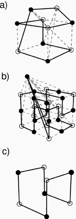
Figure 1: The construction of the lattice graphs for generation of a) Hamiltonian walk on even lattice; b) on odd lattice; c) Hamiltonian cycle. The walks are drawn as solid lines and the edges of the lattice graphs as dash lines.

From the discussion above, it may seem that generation of Hamiltonian walks on odd and even lattices, and generation of Hamiltonian cycles on even lattices, are three very different problems which should be treated separately. In fact, they can all be reduced to one another by the trick proposed in the article Conf-des . Let us introduce extended graph by adding some out-of-lattice vertices using the following rules:

• In case of even lattice, we add two out-of-lattice vertices of different colors (see Fig. 1a). We connect them to each other, and each of them - to all the lattice vertices of the opposite color.

• In case of odd lattice, we add only one out-of-lattice vertex, which is colored minor color and connected to all major color ”real” vertices (Figure 1b).

Constructed this way, extended lattices are always even. Therefore, all we have to do is to generate Hamiltonian cycles on the even lattices. As soon as that problem is addressed, we can generate Hamiltonian cycle on the extended lattice and obtain open Hamiltonian walk by just removing the out-of-lattice vertices.

II.2 The algorithm

The original combinatorial algorithm by Ramakrishnan et al Conf-des consists of two steps. First, it generates some configuration of sub-cycles and sub-chains with dead ends on the lattice by means of two-matching procedure; second, it transforms these pieces into a single Hamiltonian walk using another procedure called patching. The main novelty of our algorithm is that the formation of sub-cycles and sub-chains is forbidden, and we always generate the single Hamiltonian cycle on the extended lattice graph. Thus, patching stage becomes unnecessary. We explain in the Appendix A, why the formation of small loops and sub-chains in the original method Conf-des biases sampling of the Hamiltonian walks.

The algorithm works by placing links on the lattice graph. At the beginning, the lattice graph contains no links. Then, algorithm starts placing links randomly, connecting randomly chosen neighboring vertices (Figure 2a). Every time a new link is chosen, we check whether it forms an unwanted small subtitle or a dead end (Figure 2b), and the link is rejected if this happens. (The only little exclusion from the general rule is required for an even lattice, where the first link is always drawn between the out-of-lattice vertices, and this link is never removed on the later steps of the algorithm.) The algorithm stops when all vertices of the graph are saturated by two links each, and the links form a Hamiltonian cycle. The obvious difficulty is that randomly chosen vertex frequently cannot be linked to its randomly chosen neighbors, because the latter is already saturated (Figure 2c). This is the situation in which two-matching is applied.

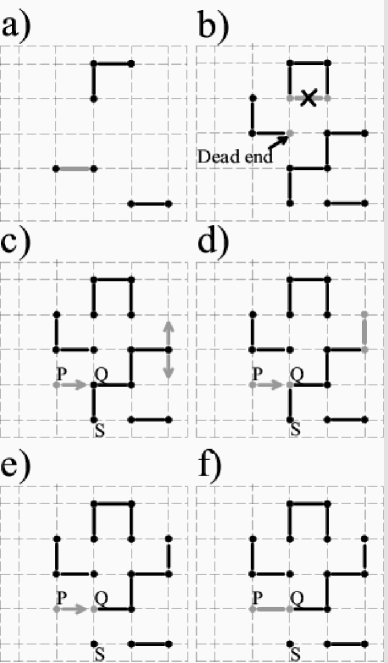
Figure 2: Schematic representation of the application of the algorithm. For simplicity, steps of the algorithm are shown in two dimensions. See text for further explanations.

Two-matching starts from picking up a vertex, $P$, which is currently either not connected, or has only one incoming link. Then, its random neighbor $Q$ is chosen as an opposite end of the new link. If $Q$ belongs to some linear sub-chain, we peak up randomly one of the links incoming to it and follow this direction along the sub-chain. When the sub-chain terminus is found, it is investigated for the possibility to be connected with one of its neighbors. For each vertex, all the non-saturated neighbors ending the sub-chain are placed on the special list. The neighbors are not included in the list if linking with them leads to the formation of sub-cycles or dead ends (Figure 2d). Then, a random vertex from the list (of course, if the list is not empty) is chosen, and the new link is drawn (Figure 2e). The growth of the sub-chain is followed by the switching of the links incident on $Q$. The link such as $QS$ (see Figure 2f; the link opposite to the one pointing to the end just elongated) is removed and the new link $PQ$ is drawn, subject to the following two conditions: i) the vertex $P$ is still unsaturated after the elongation of the sub-chain; ii) linking the vertices $P$ and $Q$ does not produce subtitle or dead end. Depending on the success of two processes contributing to the two-matching, the number of links on the graph increases by one, remains the same, or decreases by one. In our simulations, the latter case was rare and did not slow the process too much.

The new links are placed on the graph until finally a single cycle passing once and only once through every vertex of the graph (including the out-of-lattice ones) is formed.

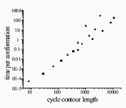
Figure 3: Performance of the algorithm for generation of Hamiltonian walks and cycles on cubic lattices. The results for even walks are shown as triangles, for odd walks as diamonds, for cycles as squares.

II.3 Algorithm performance test

We implemented the algorithm described just above to generate linear polymer chains up to the size $12\times 12\times 12$ on even lattices, up to $15\times 15\times 15$ on odd lattices, and the compact cycles of the sizes up to $22\times 22\times 22$. On the lattices larger than mentioned this algorithm becomes exponentially slow, however, for the investigated lattices, we found the CPU time necessary to generate one chain conformation demonstrates power law dependence on the length of the walk, $N$. The effectiveness of our algorithm executed on the Pentium III 1.1 GHz PC is demonstrated in Figure 3. The run time scales approximately as $N^{2.1}$ for both linear polymers and cycles for the moderate chain lengths. This is slower than performance reported in Conf-des for the original algorithm ($\sim N^{1.1}$). This is the price we must pay to ensure fair sampling. Still, our algorithm allows to generate compact polymer chains within the length range of several orders of magnitude.

II.4 Topological aspects

There exists abundant literature on computational studies of the knot composition of non-compact closed chains, starting with the pioneering work of Vologodskii et al Vologodskii ; VologodskiiReview ; Michels ; Koniaris ; Shima ; DeguchiTsuru . These studies are mostly motivated by the intent to model closed circular DNA. There are much fewer studies made with compact chains Tesi ; Mansfield , although the question of knots in proteins is widely considered a puzzle Mansfield1 ; Mansfield2 ; knotted_protein ; Nature_knots_protein .

We should particularly emphasize the work by Mansfield Mansfield , where he addressed knots in Hamiltonian cycles on the cubic lattice. What we add here to his analysis is we pull it to significantly longer loops, which turns out to be essential, and we also study the statistics of the sub-chains in the loop whose overall global topology is fixed.

As in all previous works, we applied the theory of knot invariants to determine the knot-type of a given conformation. Knot invariants are mathematical objects that serve as a ’signature’ of the knot-type. As a signature, knot invariants are, unfortunately, not unique to a given knot. The use of the appropriate types and number of knot invariants yields only a good likelihood that the knot has been identified correctly. This likelihood is high, in certain cases unity, if the number of crossings in the knot projection could be reduced to a sufficiently small number. The difficulty we have to face here is that compact conformations have typically very large numbers of crossings on the projection.

In this work, we calculated for a knot $K$ three invariants - the Alexander polynomial ($\Delta(t)_{K}$) evaluated at a certain value of $t$, ($\Delta(-1)_{K}$), the Vassiliev invariant of degree two ($v_{2}(K)$), and the Vassiliev invariant of degree three ($v_{3}(K)$) - as was also done in DeguchiTsuru . A connection is made between a conformation and its knot-type if the invariants calculated from the projection of the conformation coincide with the invariants associated with the knot-type.

In order to illustrate the necessity of topological invariants in identifying even the simplest knots, including the trivial knot (which is an unknot) we show Figure 4. In fact, the loop shown in this figure is a trefoil knot, but it is virtually impossible to realize this fact by eye.

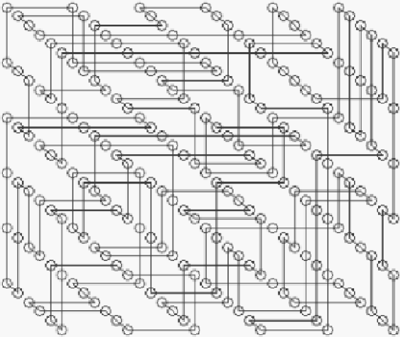
Figure 4: Projected nodes and links of a $6\times 6\times 6$ conformation. The knot formed is a trefoil.

Thus, after a compact conformation has been generated, the procedure for determining its knot-type involves the following steps: (1) Generate Plane Projection; (2) Preprocess Projection; (3) Compute Knot Invariants from Projection; (4) Match Conformation with Knot-type using Table 1.

II.4.1 Preprocessing Projection

The goal of preprocessing the projection is to simplify the knot by reducing the number of intersections or crossings of the projected links. The intuitive local ’moves’ that can accomplish this simplification are called Reidemeister moves (see, for instance, Mura ). Given the very complicated nature of typical compact conformations, we resort to combinations of Reidemeister moves, compounded, or ’macro’, as discussed in Kauffman .

For large conformations, a further simplification can be achieved by first ’inflating’ the conformation before taking the projection. A less dense conformation leads to a significant reduction of crossings. In fact, this was done for $14\times 14\times 14$ conformations before the Vassiliev invariants were evaluated.

II.4.2 Computing Knot Invariants

An algorithm for computing the Alexander polynomial $\Delta(t)_{K}$ is presented clearly in Vologodskii and will not be discussed any further here. Suffice it to say that the algorithm requires the construction of an ’Alexander’ matrix from the knot projection, with dimension equal to the number of crossings. The determinant is subsequently calculated after setting $t$ to $-1$ to obtain the single number $\Delta(-1)_{K}$.

The geometrical origin of this invariant may be traced to ’linking’ numbers calculated from a set of closed curves. These closed curves are associated with a ’Seifert surface’ whose boundary is the knot Mura .

The calculations for the Vassiliev invariants ($v_{2}(K)$,$v_{3}(K)$) are presented as diagrammatic formulas in Polyak . These formulas operate on a Gauss diagram, or equivalently on a Gauss code for a knot $K$. The set of Vassiliev invariants may be considered as a generalization of the Gauss integral formula for the linking number.

As mentioned earlier, it is possible for two distinct knots to have the same set of knot invariants. However, we expect that the false identification of a knot would be rare. For instance, the set of three knot invariants for the trivial knot is distinct from those of (prime) knots with $10$ minimum crossings or fewer ($249$ knots in all) in their projection.

Table 1: Values of knot invariants for a few knots.

KNOT	Alexander,	Vassiliev,	Vassiliev,	CHIRAL?
	$\left|\Delta(-1)_{K}\right|$	$v_{2}(K)$	$\left|v_{3}(K)\right|$
$0_{1}$	1	0	0	NO
(Trivial)
$3_{1}$	3	1	1	YES
$4_{1}$	5	-1	0	NO
$5_{1}$	5	3	5	YES
$5_{2}$	7	2	3	YES

III Results: compact chains

III.1 Statistics for the small lattices

As a first test of our algorithm, we compare the statistics of generated random samples with the results of exhaustive enumeration for $2\times 2\times 2$ and $3\times 3\times 3$ cubic lattices.

For the $2\times 2\times 2$ lattice the task is easy, because the complete list consists of only 3 symmetrically unrelated Hamiltonian walks. These walks are shown in the Figure 5. The unbiased algorithm should generate each of these 3 conformations with probabilities $1/3$. We generated samples of $100000$ walks using our algorithm and using the original algorithm of Ramakrishnan et al Conf-des . The average fractions of different walks in generated samples obtained with both algorithms are shown in Table 2. Clearly, the algorithm Conf-des fails this test; the reasons of its failure are explained in the Appendix A.

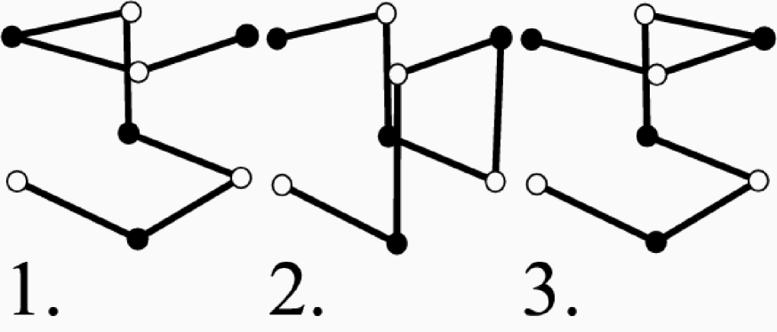
Figure 5: There are three symmetrically unrelated conformations possible on $2\times 2\times 2$ cubic lattice.

Table 2: The average fractions of different $2\times 2\times 2$ conformations in generated samples obtained with two algorithms.

	Conformation
Algorithm	1	2	3
Ramakrishnan et al Conf-des	0.278	0.358	0.364
present	0.328	0.328	0.344

For the $3\times 3\times 3$ lattice a little more elaborate procedure is necessary. Suppose, there are some $M$ conformations (for instance, $M=103346$ for $3\times 3\times 3$ lattice Shakhnovich ), and suppose we repeatedly apply one and the same algorithm to generate a number $K$ of Hamiltonian walks. Apart from glitches with the random number generators, subsequent applications of the algorithm are statistically independent. Therefore, for every conformation $i$ there is the occurrence probability $p_{i}$. For the unbiased algorithm, $p_{i}=1/M$; in general, $\epsilon_{i}=p_{i}-1/M$ measures the bias. To examine this bias, we compute the distribution $m_{k}$ - for every number of appearances $k$, $m_{k}$ is the number of conformations that appeared $k$ times in $K$ trials. Obviously, $m_{k}$ is normalized such that $\sum_{k=0}^{K}m_{k}=M$. Since appearances of every particular conformation are binomially distributed, we have

$$m_{k}=\sum_{i=1}^{M}p_{i}^{k}(1-p_{i})^{K-k}\frac{K!}{k!(K-k)!}\ ,$$ (1)

where the summation runs over all conformations. From here, it is not difficult to find that, first of all, the average (over all conformations) appearance number is $\overline{k}=K/M$, it is independent of a bias. The information about the bias is contained in further moments of the distribution. Specifically, we consider the further cumulants of the distribution of $\epsilon_{i}$: variance

$$\langle\epsilon^{2}\rangle_{cum} \equiv \langle\epsilon^{2}\rangle=$$ (2)

$$= \frac{1}{K^{2}}\left[\overline{\left(k-\overline{k}\right)^{2}}-\frac{K}{M}\right]\ ,$$

skewness

$$\langle\epsilon^{3}\rangle_{cum} \equiv \langle\epsilon^{3}\rangle=$$ (3)

$$= \frac{1}{K^{3}}\left[\overline{\left(k-\overline{k}\right)^{3}}-3\overline{\left(k-\overline{k}\right)^{2}}+2\frac{K}{M}\right]\ ,$$

and kurtosis

$$\langle\epsilon^{4}\rangle_{cum} \equiv \langle\epsilon^{4}\rangle-3\langle\epsilon^{2}\rangle^{2}=$$ (4)

$$= \frac{1}{K^{4}}\left[\overline{\left(k-\overline{k}\right)^{4}}-6\overline{\left(k-\overline{k}\right)^{3}}+\right.$$

$$\left.+11\overline{\left(k-\overline{k}\right)^{2}}-3\overline{\left(k-\overline{k}\right)^{2}}^{2}-6\frac{K}{M}\right]\ ,$$

where averaged (over all conformations) powers of $\epsilon$ are defined according to

$$\langle\epsilon^{n}\rangle=\frac{1}{M}\sum_{i=1}^{M}\epsilon_{i}^{n}$$ (5)

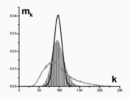
Figure 6: The computed distributions of not symmetrically related conformations on $3\times 3\times 3$ lattice by the frequency of generation obtained by our method (columns) and method of article Conf-des (grey line) compared with the distribution expected for the unbiased algorithm (black line). Here, $k$ is the number of times a conformation appeared in $K=10000000$ trials, while $m_{k}$, for every $k$, is the number of conformations which appeared $k$ times. The number of different Hamiltonian walks on $3\times 3\times 3$ lattice is $M=103346$.

We generated two samples of $K=10000000$ Hamiltonian walks by means of our algorithm and the one of the article Conf-des and compared the appearance of different Hamiltonian walks in these samples. The obtained distributions $m_{k}$ for both algorithms are shown in Fig. 6. The distribution (1) for the unbiased $\epsilon=0$ case (when it is simply a Gaussian with the mean $K/M$ and variance also $K/M$) is also presented in the same Figure. The parameters of the computed distributions are summarized in the Table 3.

Table 3: The parameters of computed distributions of conformations on $3\times 3\times 3$ lattice obtained with two algorithms.

Algorithm	$\frac{\left(\langle\epsilon^{2}\rangle_{cum}\right)^{1/2}}{1/M}$	$\frac{\left(\langle\epsilon^{3}\rangle_{cum}\right)^{1/3}}{1/M}$	$\frac{\left(\langle\epsilon^{4}\rangle_{cum}\right)^{1/4}}{1/M}$
Ramakrishnan
et al Conf-des	$0.34$	$0.34$	$0.35$
present	$0.12$	$0.09$	$0.21$

As the data indicate, our algorithm produces the distribution, which is close to the expected unbiased result. The distribution shape is very closely Gaussian, which means the bias is weak. At the same time, the algorithm of the article Conf-des showed poor results and produced the distribution, which is essentially skewed. This demonstrates strong biases of that method.

A not so good news about our algorithm is that the width of the distribution is still larger than expected for unbiased sampling. Given the width of the distribution we can estimate the bias from formula (2), $\epsilon=1.2\times 10^{-6}$. This signals certain bias, about $10\%$, in the generation of Hamiltonian walks. However, the bias is small, and certainly much smaller than for the previous algorithm. In what follows, we shall examine the statistics of Hamiltonian walks generated by our algorithm and neglecting its bias.

III.2 Statistics of segments and loops in generated walks

By the statistics of segments we understand the following. Imagine a long polymer compressed in a very compact state, and suppose a part of the chain, some $\ell$ monomers long, is labeled. For instance, it may be deuterated. Then, we can study the conformation of the labeled segment. Is it collapsed, with the overall size scaling as $\ell^{1/3}$? Is it extended, with end-to-end distance scaling as $\ell^{1}$? Does it exhibit any signs of regularity, such as helical structure of some sort? Or is it purely random, yielding Gaussian statistics with the size scaling as $\ell^{1/2}$? This is the question we want to address here.

To begin with, let us remind the major conclusions of the mean field theory (see, e.g., review in the book RedBook ). This theory suggests that labeled chain segment behaves similarly to the labeled chain in a macroscopic polymer melt or concentrated solution of different chains. Therefore, it obeys Flory theorem Flory ; Edwards ; DeGennesBook . To appreciate the highly non-trivial statement of the Flory theorem, one has to realize first of all that either labeled chain in the concentrated melt, or labeled $\ell$-segment in the globule, is subject to the volume exclusion constraint: trivially, other monomers cannot penetrate the volume occupied by any given monomer. As it is well known in polymer physics, volume exclusion leads to polymer swelling, with significant correlations between monomers, and with chain size scaling $\ell^{\nu}$, $\nu\approx 0.588\approx 3/5$. It is not difficult to realize that the presence of surrounding chains in the melt, or surrounding parts of the same chain in the globule, leads to some effective attraction between labeled monomers. Flory theorem says that this attraction exactly compensates the excluded volume effect. In other words, surrounding polymer medium shields excluded volume effect, leaving labeled chain with Gaussian statistics and the size proportional to $\ell^{1/2}$. This screening is sometimes called Edwards screening, it is similar to Debye screening in plasma.

What is the range of $\ell$ in which Gaussian scaling $\ell^{1/2}$ is expected? Of course, $\ell$ must be larger than the effective Kuhn segment - which is equal to unity for the lattice model. Another restriction, relevant for the globule and not for the melt, is that labeled segment as a whole should be away from globule boundaries, or surfaces. Assuming globule size about $N^{1/3}$ for the globule of density one and the chain of $N$ monomers, we arrive at the condition $\ell^{1/2}<N^{1/3}$, or $1<\ell<N^{2/3}$.

Although this is not very important for the present study, we would like to digress to inform the reader that even within the mean field level, there are delicate corrections to the simple picture as described above. To understand this, one should think of an auxiliary problem of a Gaussian polymer without excluded volume confined in a cavity with impermeable walls. Under such conditions, chain adopts a conformation with density peaked at the middle of the cavity and with density almost vanishing at the cavity walls RedBook . The contrast between this theoretical model and the real globule with flat distributed internal density suggests that self-consistent field acting inside the globule not only compresses the chain, acting like a cavity, but also pulls the monomers from globule center to the periphery. This pull slightly perturbs Gaussian statistics of the sub-chains, particularly those located nearby the globule boundary. Computationally, we shall not look into this delicate effect in our present study.

Thus, we compute the mean square end-to-end distances of the segments of Hamiltonian walks:

$$\langle R^{2}(\ell)\rangle=\frac{1}{K(N-\ell)}\sum_{j}^{K}\sum_{i}^{N-\ell}\left({\vec{r}}_{i+\ell}^{(j)}-{\vec{r}}_{i}^{(j)}\right)^{2}\ ,$$ (6)

where $\ell$ is the contour length of the segment of the walk (in units of steps), $K$ is the total number of walks in the sample, $N$ is the length of the walk, ${\vec{r}}_{i}^{(j)}$ is the position vector of the vertex visited $i$-th in the $j$-th walk.

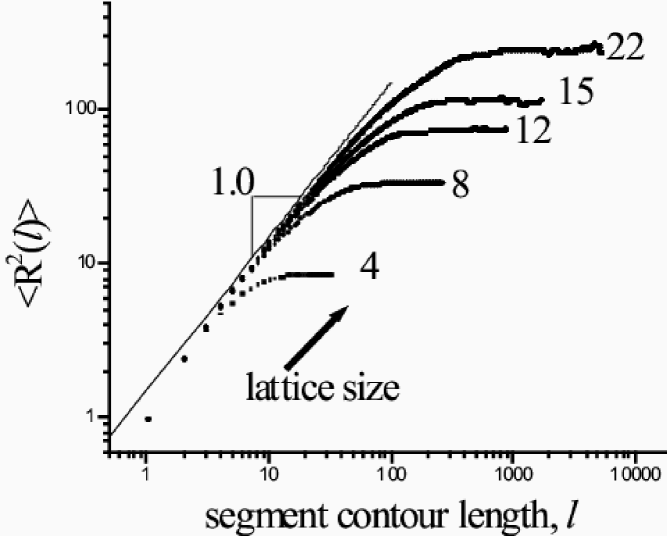
Figure 7: Mean square end-to-end distance of the segments of Hamiltonian walks vs. the lengths of segments is shown for the lattices of different sizes. The curves for linear walks and cycles on the lattices $4\times 4\times 4$, $8\times 8\times 8$ and $12\times 12\times 12$ coincide.

The results for the samples of Hamiltonian walks of different lengths are presented in Figure 7. In good agreement with mean field theory, on the scales smaller than $N^{2/3}$ the walks obey Flory theorem Flory and the average distance between the segment ends scales such that $\langle R^{2}(\ell)\rangle\sim\ell$. We would like to note here that Flory theorem does not tell us anything about the prefactor of this scaling. Fitting on the statistics of the lattice polymer cycles of the size $22\times 22\times 22$ suggests the prefactor to be equal $\approx 1.5>1$. For the polymer chain without excluded volume it is exactly equal to $1$. Therefore, the excluded volume effectively increases the Kuhn segment length.

On the scales $\ell\sim N$, the walk starts feeling the confinement by the lattice borders, and $\langle R^{2}(\ell)\rangle$ levels off.

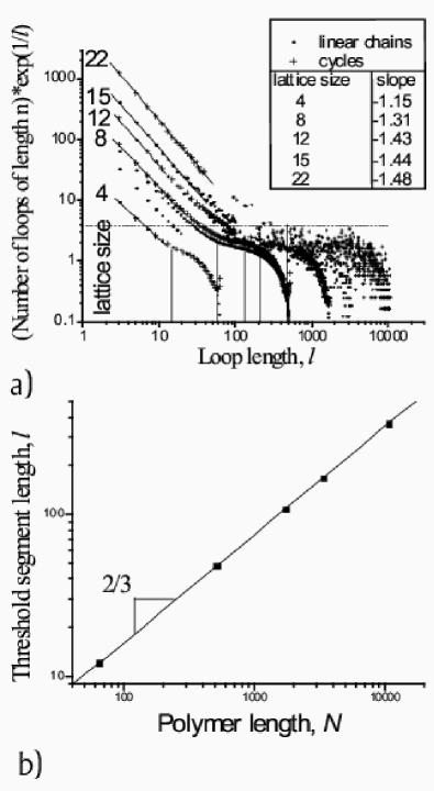
Figure 8: (a)The average number of loops of various contour length in generated Hamiltonian walks on the lattices of different size. Vertical lines display the cross-over values of $\ell$ at which looping probability saturates. Horizontal dash line corresponds to the predicted saturation level for the $22\times 22\times 22$ walks. (b) The dependence of the cross-over value of $\ell$ on the polymer length.

Another measure of the agreement between statistics of Hamiltonian walks and Flory theorem is the looping probability. The Figure 8a shows how often the loops of different contour lengths appear in the Hamiltonian walks. Here, we say that the walk makes a loop of the length $\ell$, if after visiting site with the coordinates ${\vec{r}}_{i}$ it visits one of this site neighbors in exactly $\ell$ steps. What does the mean field theory have to say about these loops?

As we saw for the statistics of end-to-end distances, on the scales $\ell<N^{2/3}$, the Hamiltonian walks are Gaussian. Then, the probability distribution of their end-to-end vectors ${\vec{R}}$ must obey Gaussian law $\sim\ell^{-3/2}\exp\left[-{\vec{R}}^{2}/\ell\right]$. For the loop, $R=1$. Therefore, average number of loops of the contour length $\ell$ should decay as $\ell^{-3/2}\exp(-1/\ell)$ with growing $\ell$. That is why the number of loops on the vertical axis of the Figure 8a is weighted by the factor of $\exp(-1/\ell)$. We can express surprise that power law $\ell^{-3/2}$ comes so slowly and appears only at large $N$ (see the table on the inset to Fig. 8a).

We can also check cross-over value of $\ell$ and how it depends on $N$. Vertical lines on the Figure 8a mark the characteristic segment lengths at which the cross-over takes place for the polymer chains of different length. And Figure 8b shows the dependency of these threshold values on the polymer length $N$. It is clearly seen that $\ell$ scales as $N^{2/3}$.

On the larger scales, $\ell>N^{2/3}$, the probability to find the loop of length $\ell$ saturates and becomes practically independent of $\ell$. To estimate its constant value, we can resort to the following argument. The random walk of a length greater than $N^{2/3}$ hits the borders of the lattice. The end of the longer walk may be found in any lattice site with nearly equal probability $1/N$. Since the loop formation condition is met by $\langle z\rangle$ of sites neighboring to the loop starting site, the loop probability is about $\sim\left.\langle z\rangle\right/N$. Here, $\langle z\rangle$ is the mean coordination number of the lattice (which takes into account that the sites on the surface have fewer neighbors than those in the bulk). At the same time, there are $N-N^{2/3}\approx N$ such loops possible, therefore, there must be about $\langle z\rangle$ loops of each length found in every walk. Indeed, the horizontal dash line on the Figure 8a corresponding to $\langle z\rangle$ of the compact walk of the size $22\times 22\times 22$ reasonably estimates the number of long loops in the globule of this size.

The results presented in Figure 8 are in full agreement with the theory, both in terms of the power law decay ($\ell^{-3/2}$) at moderate $\ell$, the range of the cross-over ($\ell\sim N^{2/3}$), and the constant levels at large $\ell$ ($\langle z\rangle$).

III.3 Correlation between ends in Hamiltonian walks

It is an interesting question in the theory of polymer globules, whether the ends of the polymer chain are effectively independent of each other in terms of their positions inside globules, or they repel (attract) due to the conditions of the connectedness and compactness of the chain. If the end of the chain is located in the bulk of the globule, there may be entropic cost associated with the rearrangement of the parts of the chain surrounding it due to necessity to keep the compactness of the globule. This local rearrangement of the polymer chain may affect the probability of the other end to locate in the vicinity. Effectively, this may lead either to the attraction, or to the repulsion of the ends of the chain. Theoretically, this issue remains currently unclear KardarOrland .

To check on the existence of such effective interaction between chain ends, we calculate the end-end correlation coefficient for the samples of generated Hamiltonian walks. This quantity is defined via the formula

$$c=\frac{\langle x_{1}x_{2}\rangle}{\sqrt{\langle x_{1}^{2}\rangle\langle x_{2}^{2}\rangle}},$$ (7)

where $x_{1}$ and $x_{2}$ are the $x$-coordinates of the two chain ends, $\langle\ldots\rangle$ means averaging over all sampled walks. For simplicity, we place coordinate system origin in the center of the cube, such that $\langle x_{1}\rangle=\langle x_{2}\rangle=0$. Due to the symmetry, correlations coefficients for $y$ and $z$ coordinates are the same as for $x$, while all the non diagonal elements (such as $\langle x_{1}y_{2}\rangle$ etc.) vanish.

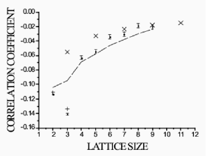
Figure 9: Mean diagonal end-end correlation coefficients for the Hamiltonian walks on the lattices of different sizes. The data of exact calculation for $2\times 2\times 2$ and $3\times 3\times 3$ lattices are shown as $+$. The data of exact calculation of correlation coefficients for the random pairs of dots on the odd lattices obeying the excluded volume condition and the chess board theorem are shown for the comparison as $\times$. The results obtained from generation of the walks with algorithm of the work Conf-des are shown as the dashed line.

The results obtained from the simulations on the lattices of the size $L=2,3,\ldots,10$ are presented in Figure 9 along with the data of the exhaustive enumeration for the $2\times 2\times 2$ and $3\times 3\times 3$ lattices and the exact results for the disconnected ends model (which, due to the chess board theorem, is only meaningful for odd lattices; for even lattices, two ends must be on the oppositely colored sites, and, therefore, are not correlated at all). The results for the small lattices are very close to exact (whereas the original algorithm Conf-des produces significant systematic errors). This is another good suggestion that our algorithm has weaker bias than that of the work Conf-des .

The fact that correlation coefficient is negative indicates that there is some effective repulsion between the chain ends. This effect decreases and supposedly goes to zero with increasing of lattice size. Moreover, correlation between ends very rapidly approaches correlation between disconnected points subject only to excluded volume condition. This observation suggests that even the small repulsive correlation between chain ends is mostly due to the benign excluded volume effect of the terminal monomers, and chain connectivity provides only faint, although also repulsive, contribution (probably mostly due to excluded volume of monomers next to the terminal ones).

IV Results: compact loops and their knots

IV.1 Average Crossing Number

Figure 10 displays the average number of crossings in the plane projection of a conformation, together with the reduced number and mathematical prediction, for the range of sizes $L=4$ to $L=20$. The crossing numbers are plotted against the length (number of monomers) $N=L^{3}$.

The prediction

$$C=\left(\frac{L^{3}}{3(L-1)^{2}}-1\right)\frac{L^{3}}{3}$$ (8)

for the average crossing number of an $L\times L\times L$ conformation follows from the assumption that every segment upon projection in some ’vertical’ direction produces crossings with all segments above and below it inside the cylinder of the cross-section unity. In this sense, the result for the average crossing number is trivial. However, it is interesting to note that for large $L$, the expression for the average crossing number scales as $C=L^{4}=N^{\frac{4}{3}}$, which is reminiscent of a ’four-thirds power law’ relating crossing number and ’rope length’ for tight knots Buck96 ; Canta ; BuckNature . This suggests that this four-thirds power law does not reflect on any intimate properties of tight knots, except their overall space filling character.

From the average crossing number, one could get an idea of how the amount of computational resources involved in the calculation of a knot invariant, say Alexander, scales with conformation size. The Alexander invariant entails computation of the determinant of a $C\times C$ matrix. Naively using Gaussian elimination, computation time would roughly scale as $C^{3}=N^{4}$.

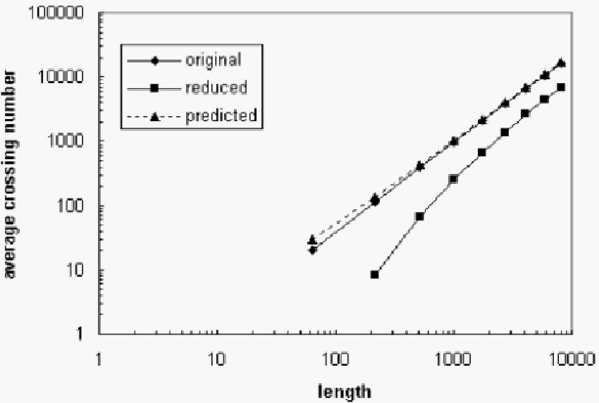
Figure 10: Average crossing numbers in the knot projection, before and after preprocessing with Reidemeister moves, together with mathematical prediction. These were plotted against the size (length $N=L^{3}$) of the conformation, from $L=4$ to $L=20$.

IV.2 Knot Probabilities

Figure 11 displays our results for the fraction of conformations (of a given size $N=L^{3}$) which are unknotted. For each $L$ from $4$ to $12$, $10^{5}$ conformations were generated. The last data point for the largest conformation we were able to analyze ($14\times 14\times 14$) represents $4$ trivial knots out of $350000$ conformations.

Since the total number of conformations of the length $N$ grows exponentially with $N$, it is not a surprise that the probability of a trivial knot decays exponentially with $N$ theorem1 ; theorem2 . Accordingly, computational data on trivial knot probability are customary fit to exponential. In our case, the exponential fit to the (last three) data points yielded an estimate for the unknotting probability as a function of $N$, $\sim\exp(-N/196)$, as shown in Figure 11.

Previously, there were some works measuring knotting probabilities for lattice polygons in confined geometries Tesi ; Mansfield . In particular, Mansfield Mansfield has examined knots of compact Hamiltonian cycles on a lattice - the same problem we consider here. However, these authors use one invariant, the Alexander polynomial, in their computations (although Mansfield Mansfield evaluated Alexander polynomial at $10$ different values of $t$). This is understandable, as the Vassiliev invariants are a relatively recent discovery Polyak , in particular the invention of explicit and computationally implementable formulas for their evaluation. Moreover, we were able to analyze larger conformations: the work Mansfield examined $N\leq 1000$, while we consider $N$ up to $14^{3}=2744$, almost three times larger.

Mansfield’s fit to his results ($\exp(-N/270)$) is shown in the thinner, dotted line in Figure 11. Importantly, our results for $N\leq 1000$ agree well with both the results and the fit by Mansfield Mansfield . However, examination of larger $N$ leads us to revise the estimation of characteristic length $N_{0}$ in $\exp(-N/N_{0})$ from $N_{0}\approx 270$ to $N_{0}\approx 196$. Moreover, our result for $N_{0}$ may turn out an overestimate, and real $N_{0}$ may eventually be found even smaller than $200$. Indeed, the leading source of inaccuracy in our results is due to the incomplete set of topological invariants. This can lead to errors of assigning the trivial knot status to some loops which are in fact not trivial knots. Such errors contaminate our trivial knot sets with non-trivial knots, leading to the overestimate of trivial knot probability, and this effect only increases with growing $N$, because at small $N$ it is much less likely to meet a non-trivial knot confused with trivial one by our set of knot invariants. Thus, we conclude that the trivial knot probability for compact polymers goes as

$$w_{\rm compact,\ trivial}\simeq\exp\left(-N/N_{0}\right)\ ,\ \ \ \ \ N_{0}\lesssim 196\ .$$ (9)

This result is essential for several reasons. We have shown in the section III.2 that the sub-chains inside the sufficiently big compact globule behave somewhat like Gaussian polymers, with $R^{2}(\ell)$ proportional to $\ell$ despite the obvious presence of volume exclusion constraint. This fact, consistent with Flory theorem, leads to the traditional understanding that the chains in the melt as well as sub-chains in the globule are Gaussian. From this, it would then be logical to assume that the trivial knot probability for them should also be the same as for corresponding Gaussian polymers, and not the same as for the swollen self-avoiding polymers. We remind that the trivial knot probability for Gaussian polymers, that is, for polygons of $N$ segments with no volume exclusion, also follows the exponential law $\exp(-N/N_{0})$, with $N_{0}$ varying from about $350$ for Gaussian random polygons (in which all segments have Gaussian distributed lengths) DeguchiTsuru to about $260$ for regular polygons (made of length $1$ segments) Koniaris ; Nathan . For the self-avoiding polymers, the value of $N_{0}$ is even larger Shima ; EXP(-28) . Our result now indicates that in regard to the knot forming ability of the polymer, chain compaction not only screens away the excluded volume, reducing $N_{0}$ from its value for ”thick” polymers to that for ”thin” ones, but produces the much more dramatic effect, decreasing $N_{0}$ significantly below its Gaussian value. In brief, compact polymers, although they satisfy Flory theorem, are not Gaussian for topological purposes, they are much (exponentially) more prone to forming knots.

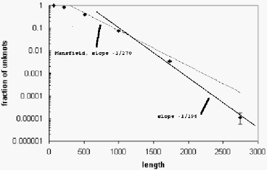
Figure 11: Trivial knot probabilities for conformations of size $L=4$ to $L=14$. The thinner dotted line represents Mansfield’s Mansfield fit to his data points.

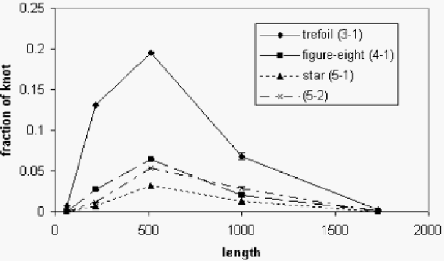
Figure 12: Probabilities of occurrence of a few knots.

The Figure 12 displays the probabilities of some non-trivial knots in compact loops as the function of the loop length. Similar to the studies made with non-compact chain models (see, e.g., DeguchiTsuru ; Shima ), the probability to obtain any particular knot starts from $0$ at small $N$, then reaches a maximum at some finite value of $N$, and then decreases and asymptotically approaches to $0$ with further growth of $N$. As in other cases, the qualitative explanation of this tendency is clear. When $N$ is small, the loop might be too short to form a given knot. In fact, for the lattice model, it is clear that for every knot there is a finite value of $N$ below which this knot cannot be formed at all, so its probability is exactly $0$ (for instance, the shortest loop capable of forming a non-trivial knot on the cubic lattice has $N=24$ segments). However, even for significantly larger $N$ there might still be relatively few conformations to realize the given knot, and that yields low probability. At the other end, when $N$ is exceedingly large, there are great many knots which can be comfortably formed, and their number keeps increasing with $N$, yielding a decaying probability to locate the given knot. We should emphasize that the results presented in Figure 12, although qualitatively reasonable, have somewhat preliminary character, because our use of the restricted set of topological invariants at the very high crossing numbers may lead to inaccurate knot assignments.

IV.3 Statistics of segments and loops in trivial knots

In this section, we want to address the following problem. Consider a sub-chain of some length $\ell$ which is large, but much smaller (in a proper sense) than the entire globule. Suppose further that the chain as a whole is closed, so it is a loop, and that this loop is a trivial knot. On the one hand, since $\ell\ll N$, it seems that the sub-chain has no way to ”know” what are the global topological properties of the entire loop. On the other hand, it is also obvious that the property of being a trivial knot is not a local but a global property of the loop. In some loose sense, we can say that since the entire loop has no knots, there is no way the sub-chain of the length $\ell\ll N$ may have knots. Of course, to speak about knots in a sub-chain we should somehow decide how to close its ends; what we are saying here is that the sub-chain of an unknotted loop must not have knots under the majority of natural ways to connect its ends. This logic then seems to suggest that the sub-chain may tend to be swollen compared to its random walk size $\ell^{1/2}$, based on the analogy with loops in unrestricted space in which trivial knots are known to swell Shima ; Nathan ; 3_5_uzla . However attractive, this logic at least does not exhaust the problem, because if sub-chain sizes were to scale as $\ell^{\mu}$ with $\mu\geq 1/2$, then these sub-chains would strongly overlap in the overall compact globule, making it difficult to avoid making knots between the sub-chains. All these inconclusive arguments are presented here in order to motivate the problem: how does the sub-chain size (say, end-to-end distance) scale with the sub-chain length if the sub-chain is buried deeply inside a collapse trivial knot?

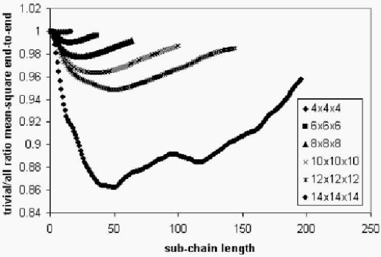
Figure 13: Ratio of sub-chain mean-square end-to-end distance in trivial knots and in all loops versus number of links in the sub-chain. For the chain of the length $N=L^{3}$, filling $L\times L\times L$ cube, results were plotted up to $L^{2}$.

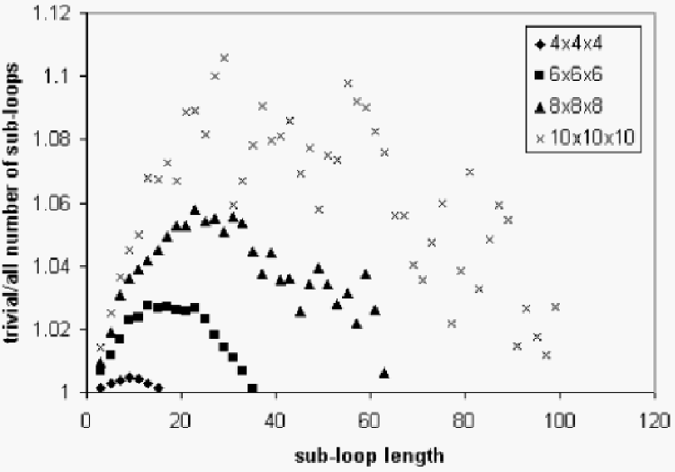
Figure 14: Ratio of number of sub-loops in trivial knots and in all loops, versus number of links in the sub-loop. Results for $L=12$ and $L=14$ were not plotted due to excessive ’noise’. This result complements figure 13.

Measurements of mean-square end-to-end distance (defined similarly to Eq. (6)) were made on sub-chains (segments) of compact chain conformations with trivial knots and on sub-chains of all conformations regardless of knot-type. The results (figure 13) show that sub-chains of trivial knots are smaller or more compact compared to sub-chains of all knots. A similar result was also obtained for the gyration radius, which is another measure of size. (The extrema in the plots are, of course, effects of the finite size of the conformations.)

Measurements of the number of sub-loops formed in each conformation were also made (Figure 14. A loop is formed when monomers not connected by a link are next to each other in space). The result for the number of sub-loops in conformations with trivial knots, compared to the number of sub-loops in conformations regardless of knot-type, is in complete agreement with the previous results: since sub-chains are more compact in overall trivial knots, they are more likely to form sub-loops.

These results should be contrasted to the corresponding results for gyration radius of (entire) non-compact rings, which indicate that trivial knots in such rings are, on average, larger compared to all other knots Shima ; Nathan . This is understood 3_5_uzla based on the argument that there are very compact conformations available for non-trivial knots are included in the average over all loops and are excluded from the average over trivial knots only. Clearly, for this ensemble of unrestricted loops, trivial knots remain swollen compared to the all-loops-average not only on the level of entire polymer, but also on the level of the sub-chains. In fact, this effect is expected to be scale-invariant at the length exceeding the characteristic knotting length $N_{0}$ 3_5_uzla . Based on this comparison, we can conclude that it must be significantly more difficult to confine a trivial knot loop into a small volume than to realize a similar confinement of a phantom polymer, either a chain or a loop. Indeed, to compress a trivial knot one has to reduce its entropy by forcing all the sub-chains to shrink. This means, confinement entropy for the trivial knot is a volume effect, it scales as $N$ in thermodynamic limit. It must be compared with confinement entropy of usual polymers which only scales as $N^{2/3}$ RedBook . This conclusion of the increased stiffness of trivial knots compared to other loops is consistent with the data of the work Nathan on the probability distributions of the unrestricted loop sizes: with decreasing overall loop size, this probability decreases much sharper for trivial knots than for averaged loops.

Although short of a proof, our results are consistent with the hypothesis of a ”crumpled globule,” which was formulated many years ago crumpled , and which remains in the rank of hypothesis till today.

V Conclusion

We formulated the new combinatorial algorithm for generation of Hamiltonian walks and cycles on the cubic lattices. This algorithm reduces biases compared to the previously known methods. The presented algorithm performs well on generation of the large compact self-avoiding walks.

We employed the proposed generation algorithm to verify Flory theorem in its applicability to the random compact chains. We found that the statistics of the sub-chains inside the large globule approaches Gaussian, as predicted by Flory theorem, for sufficiently long polymers. Unexpectedly, this happens at rather large values of chain length $N$, about $10^{5}$. Although it is not entirely clear what is the most reasonable numerical correspondence between $N$ for the lattice toy model and the number of residues a the real protein, it is safe to question the direct applicability of Gaussian statistics for the interior of even large protein globules. On the other hand, it should be understood that the deviations from Gaussian statistics found for modest $N$ compact chains are really small, and unless one is interested in sophisticated scaling analysis, they provide very reasonable qualitative fit to the data.

Using knot invariants, we were able to identify the trivial knots and the first few knots in a sample of loop conformations. We found that the probability of trivial knot in a compact conformation is significantly smaller than was previously believed, and that it is much smaller than for the corresponding Gaussian polymer. This suggests that there should be an abundance of knots in a random sample of compact conformations. We have also found that global restriction that the loop as a whole is a trivial knot has a dramatic statistical effect on the conformations of all sub-chains, making them significantly more compact than for other loops.

Our results suggest that low propensity of knots in real proteins might in fact be a statistically significant fact requiring an explanation, although it seems too early to speculate what this explanation might be, whether it is related to the physics of folding, or to some functional properties of proteins, or to some aspect of their evolution.

Appendix A Is the new combinatorial algorithm unbiased?

The building of the Hamiltonian walk on the lattice with the help of some combinatorial algorithm can be viewed as the process of labeling the edges of the lattice according to some rules (as two matching, patching or other procedures). One of the rules is that none of the lattice nodes may have more then two labeled edges incident on it. There are different configurations of the labeled edges possible on the lattice. We now would like to consider the space of all the possible such configurations. Such space itself can be represented as a graph, in which every configuration of labeled edges is a vertex, and two vertices are connected if and only if the corresponding configurations differ only by the labels of one lattice edge. Such space includes configuration in which none of the edges is labeled. We call such a configuration root. The space can be divided into the following subspaces:
i) configurations of labeled edges at which some of the lattice nodes do not have incoming labeled edges (disconnected nodes);
ii) configurations containing multiple sub-cycles and sub-chains, all the lattice nodes have two incident labeled edges except the ends of the sub-chains. No new lattice edge can be labeled. (Such configurations the algorithm Conf-des used to start patching procedure);
iii) Hamiltonian cycles.
The configuration space is schematically shown in the Figure 9. As an illustration we display different configurations possible on the extended $2\times 2\times 2$ lattice.

An arbitrary combinatorial algorithm building a Hamiltonian walk starts from the root node of the configuration space graph, then performs random walk along some path on the graph, and finishes its work at some node of subspace (iii). For the algorithm to be unbiased, the number of all possible paths leading to each node in the subspace (iii) should be equal.

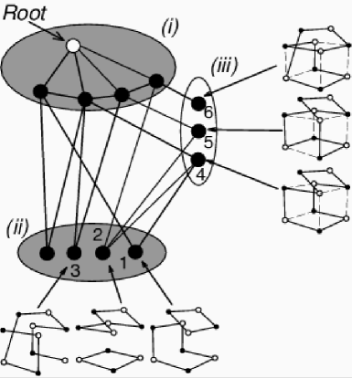
Figure 15: The space of possible configurations of links on the cubic lattice. Different subspaces and example configurations of links are shown.

Let us consider the procedures of labeling random links, branching and patching of algorithm Conf-des . The random labeling of links and branching of sub-chains may lead either directly to the formation of the Hamiltonian cycle from subspace (iii), or to the formation of some configuration from the subspace (ii). The latter situation is much more probable due to the size of the subspace (ii) is much larger than the size of (iii). Suppose the algorithm generated some configuration from (ii). Now the patching procedure has to transform it to the single cycle. Even if one supposes that configurations from (ii) and (iii) are generated with equal probability, it appears that the number of paths leading from (ii) to different Hamiltonian cycles in (iii) is different. This can be easily seen from the enumeration of all possible ways to label the $2\times 2\times 2$ lattice. The configurations 1 and 2 can be transformed to the Hamiltonian cycles 4 and 5, but there is no way to obtain the cycle 6 as a result of patching. Moreover, the number of paths to cycles 4 and 5 is also slightly different. In general, the probability to generate some Hamiltonian walk is proportional to the number of possible configurations of sub-cycles which can be transformed to this walk and to the number of ways to apply patching procedures to these configurations of sub-cycles. And this is the patching procedure that leads to the biased sampling of Hamiltonian walk. Figure 15 gives a simple example.

Also it can be shown that the formation of the configuration with dead ends (similar to the configuration 3 in Fig. 15) produces biased sampling of Hamiltonian walks too. The dead end forms if some vertex of the lattice which has only one incoming link has no unsaturated neighbors.

The algorithm Conf-des can be corrected by avoiding, on all stages, placing a new link if it leads to either the closing of a sub-cycle, or the formation of the dead ends. If the formation of the sub-cycles and the dead ends is forbidden, then paths starting from the root configuration and ending in the subspace (iii) do not pass through the subspace (ii), and the patching is not applied.

Undoubtedly, placing the links on the lattice in random order does not produce any biases. As for the branching of the sub-chains we are not so sure. However, in our simulations we did not see any worrisome signs from this procedure.

Appendix B Pseudocode

Input:	A lattice graph $LG($vertices $V$,edges $E)$.
Output:	Case 1: Hamiltonian cycle WE on the extended lattice graph;
	Case 2: (If $LG$ is even):Hamiltonian cycle $WL$ on $LG$.
Begin;
	Color vertices of $LG$ alternatively white and black;
	(if Case 1): Generate extended lattice graph $EG$;
	$PerformRandomBipartiteMatching();$
End.
Subroutines:
	$PerformRandomBipartiteMatching():$
	Begin;
		While(number of unsaturated vertices $>0$)
			Choose random unsaturated vertex $P$;
			Choose random neighbor $Q$;
			if ($Q$ unsaturated):
				$TryLinkVertices(P,Q)$;
			else if ($Q$ saturated):
				Choose direction along sub-chain, $QS$;
				Find end of sub-chain, $T$;
				$TryGrowSubchain(T)$;
				Remove link $QR$;
				$TryLinkVertices(P,Q)$;
			End if;
		End while;
	End.

$TryLinkVertices(P,Q)$:
Begin;
	Draw link $PQ$;
	Find dead ends and cycles;
	if dead ends found, or (length of cycle $<$ length of complete Hamiltonian walk):
		Remove link $PQ$;
End.
$TryGrowSubchain(T)$;
Begin;
	List unsaturated neighbors of $T$;
	While List is not empty:
		Choose random vertex $X$ from List;
		$TryLinkVertices(X,T)$;
		if link $XT$ is drawn:
			End.
		else:
			Remove link $X$ from List;
	End while;
End.

References

- (1) R. Ramakrishnan, J. F. Pekny, J. M. Caruthers, J. Chem. Phys. 103(17) 7592 (1995)
- (2) U. Mayor, N. Guydosh, C. Johnson, J. Günter Grossmann, S. Sato, G. Jas, S. Freund, D. Alonso, V. Daggett, A. Fersht Nature 421(6925) 863-867 (2003)
- (3) E. Rhoades, E. Gussakovsky, G. Haran Proc. Nat. Ac. Sci. 100(6) 3197-3202 (2003)
- (4) B. Schuler, E. Lipman, W. Eaton Nature 419(6908) 743-748 (2002)
- (5) J. Shimada, E. Kussell, E. Shakhnovich J. Molec. Biol. 308 79-95 (2001)
- (6) J. Shimada, E. Shakhnovich Proc. Natl. Acad. Sci. 99 11175-11180 (2002)
- (7) D. Klimov, D. Thirumalai Proc. Natl. Acad. Sci. 97 2544-2549 (2000)
- (8) C. Snow, H. Nguyen, V. Pande, M. Gruebele Nature 420 (6911) 102-106 (2002)
- (9) J. Ponder, D. Case ”Force Fields for Protein Simulations,” preprint, 2003
- (10) N.-V. Buchete, J. E. Straub, and D. Thirumalai Journal of Chemical Physics 118, n. 16, pp. 7658-7671, 2003.
- (11) D. K. Klimov, D. Thirumalai Journal of Computational Chemistry 23, n. 1, 161-165 (2002)
- (12) D. Gordon, G. Hom, S. Mayo, N. Pierce Journal of Computational Chemistry 24, n. 2, 232-243 (2003)
- (13) J. Karanicolas, C.L. Brooks III Proc. Natl. Acad. Sci. 100, n. 7, 3954-3959 (2003)
- (14) H. Nguyen, M. Jäger, A. Moretto, M. Gruebele, J. Kelley Proc. Natl. Acad. Sci. 100, n. 7, 3948-3953 (2003)
- (15) V. Pande Proc. Natl. Acad. Sci. 100, n. 7, 3955-3956 (2003)
- (16) H.Edelsbrunner, P. Koehl Proc. Natl. Acad. Sci. 100, n. 5, 2203-2208 (2003)
- (17) P. Rogen, B. Fain Proc. Natl. Acad. Sci. 100, n. 1, 119-124 (2003)
- (18) R. Du, A.Yu. Grosberg, T. Tanaka Physical Review Letters 84, n. 8, 1828-1831, 2000.
- (19) R. Du, A.Yu. Grosberg, T. Tanaka, M. Rubinstein Physical Review Letters 84, n. 11, 2417-2420, 2000.
- (20) E. Kussell, J. Shimada, E. Shakhnovich cond-mat/0103038
- (21) E. Kussell, J. Shimada, E. Shakhnovich cond-mat/0108357
- (22) M. Mansfield Nature Struct. Biol. 1, 213-214 (1994)
- (23) M. Mansfield Nature Struct. Biol. 4, 116-117 (1997)
- (24) W. Taylor Nature 406(6798) 916 - 919 (2000)
- (25) W. Taylor, K. Lin Nature 421(6918) 25 (2003)
- (26) A. Yu. Grosberg, A. R. Khokhlov, Statistical Physics of Macromolecules, AIP Press, New York, (1994)
- (27) D. P. Yee, H. S. Chan, T. F. Havel, K. A. Dill, J. Mol. Biol., 241(4) 557-573 (1994)
- (28) A. Maritan, C. Micheletti, A. Trovato, J. R. Banavar, Nature 406(6793) 287-290 (2000)
- (29) J. Banavar, A. Maritan Reviews of Modern Physics 75, n. 1, 23-34 (2003)
- (30) E. Shakhnovich, A. Gutin, J. Chem. Phys. 93 5967 (1990)
- (31) V.S. Pande, C. Joerg, A.Yu. Grosberg, T. Tanaka, J. Phys. A: Math. Gen. 27(18) 6231-6236 (1994)
- (32) Markov Chains and Monte Carlo Calculations in Polymer Science, Monographs in Macromolecular Chemistry, edited by G. G. Lowry, Marcel-Dekker, New York, (1970)
- (33) A. Kloczkowski, R. L. Jernigan, J. Chem. Phys. 109(12) 5134-5146 (1998)
- (34) A. Kloczkowski, R. L. Jernigan, J. Chem. Phys. 109(12) 5147-5159 (1998)
- (35) A. Kloczkowski, R. L. Jernigan, Macromolecules 30(21) 6691-6694 (1997)
- (36) A.V. Vologodskii, A.V. Lukashin, M.D. Frank-Kamenetskii, and V.V. Anshelevich, Zh. Eksp. Fiz. 66, 2153 (1974); Sov. Phys. JETP 39, 1059 (1974).
- (37) A.V.Vologodskii, M.D.Frank-Kamenetskii Sov. Phys. Uspekhi 134 641 (1981); A.V.Vologodskii Topology and Physics of Circular DNA, CRC Press, Boca Raton, 1992.
- (38) J.P.J. Michels and F.W. Wiegel, Phys Lett. 90A, 381 (1982).
- (39) K. Koniaris and M. Muthukumar, Phys. Rev. Lett. 66, 2211 (1991).
- (40) M.K. Shimamura and T. Deguchi, Phys. Rev. E 64, 020801 (2001).
- (41) T. Deguchi and K. Tsurusaki in Lectures at Knots 96, edited by S. Suzuki (World Scientific Publ. Co., 1997), pp. 95-102.
- (42) M.C. Tesi, E.J. Janse van Rensburg, E. Orlandini, and S.G. Whittington, J. Phys. A: Math Gen. 27, 347-360 (1994).
- (43) M.L. Mansfield, Macromolecules 27, 5924-5926 (1994)
- (44) K. Murasugi, Knot Theory and Its Applications (Birkhauser, Boston 1996), Chapters 5 and 6.
- (45) L.H. Kauffman in Lectures at Knots 96, edited by S. Suzuki (World Scientific Publ. Co., 1997).
- (46) M. Polyak and O. Viro, Int Math. Res. Not. No. 11, 445 (1994)
- (47) P.Flory, Principles of Polymer Chemistry, Cornell University Press, Ithaca,(1953)
- (48) M. Doi, S. F. Edwards The Theory of Polymer Dynamics, Clarendon, Oxford, 1986
- (49) P.-G. De Gennes Scaling Concepts in Polymer Physics, Cornell Univ. Press, Ithaca, 1979
- (50) M.Kardar, H.Orland (private communication)
- (51) G. Buck and J. Simon in Lectures at Knots 96, edited by S. Suzuki (World Scientific Publ. Co., 1997), pp. 219-234.
- (52) J. Cantarella, R.B. Kusner, and J.M. Sullivan, Nature, 392, pp. 237-238 (1998).
- (53) G. Buck, Nature, 392, pp. 238-239 (1998).
- (54) D.W.Sumners, S.G.Whittington Journal of Physics A: Math.& Gen., 21, 1689, (1988)
- (55) N.Pippenger Disc. Appl. Math., 25 273 (1989)
- (56) N. Moore, R. Lua, A. Grosberg (to be published)
- (57) K.V.Klenin, A.V.Vologodskii, V.V.Anshelevich, A.M.Dykhne, M.D.Frank-Kamenetskii J. Biomol. Struct. Dyn. 5 1173-1185 (1988)
- (58) A.Yu. Grosberg Physical Review Letters 85, n. 18, 3858-3861 (2000)
- (59) A.Yu.Grosberg, S.K.Nechaev, E.I.Shakhnovich Biofizika (Moscow) 23, n. 2, 265-272 (1988); A.Yu.Grosberg, S.K.Nechaev, E.I.Shakhnovich Le Journal de Physique (France) 49, n. 11, 2095-2100 (1988)