Self-consistent approach for calculations of exciton binding energy in quantum wells

Abstract

We introduce a computationally efficient approach to calculating the characteristics of excitons in quantum wells. In this approach we derive a system of self-consistent equations describing the motion of an electron-hole pair. The motion in the growth direction of the quantum well in this approach is separated from the in-plane motion, but each of them occurs in modified potentials found self-consistently. The approach is applied to shallow quantum wells, for which we obtained an analytical expression for the exciton binding energy and the ground state eigenfunction. Our results are in excellent agreement with standard variational calculations, while require reduced computational effort.

I Introduction

Excitons play an important role in the band edge optical properties of low-dimensional semiconductor structures such as quantum wells, quantum wires, and quantum dots.Harrison (1999) Quantum confinement of electrons and holes in such structures results in increased binding energy of excitons, their oscillator strength, and a life-time. As a result, excitons, for instance, in quantum wells, are observed even at room temperatures, and play, therefore, a crucial role in various optoelectronic applications.Burstein and Weisbuch (1995); Mendez and von Klitzing (1989); Nolte (1999) To be able to calculate effectively and accurately exciton binding energies in the quantum heterostructures is an important problem, and therefore, a great deal of attention has been paid to it during several decades.Miller et al. (1981); Bastard et al. (1982); Greene et al. (1984); Efros (1986); Andreani and Pasquarello (1990); Gerlach et al. (1998); Iotti and Andreani (1997); Kossut et al. (1997); Harrison et al. (1996); de Leon and Laikhtman (2000); Ekenberg and Altarelli (1987); Chang et al. (1988); Warnock et al. (1993); Piorek et al. (1995); Voliotis et al. (1995); Stahl and Balslev (1987); Balslev et al. (1989); Merbach et al. (1998); Castella and Wilkins (1998) However, this problem is rather complicated, and while significant progress has been achieved, new material systems and new type of applications require more flexible, accurate and effective methods.

Presently, the best results are usually obtained within the framework of the variational approach, where a certain form of the exciton wave function, depending on one or more variational parameters is being postulated. The exciton energy is then calculated by minimizing the respective energy functional with respect to the variational parameters. Unfortunately, even in the simplest (and, therefore, less accurate) realization of this approach it is not possible to express a value of the binding energy as a function of quantum well parameters. The best one can hope for is to obtain a set of complicated equations, which relate material parameters to several variational parameters. The latter are found numerically, and then used for numerical computation of the exciton energy. These difficulties result from the fact that variables in the Hamiltonian describing relative motion of the electron-hole pair cannot be separated: the presence of the quantum well potential breaks the translational invariance of the system, making it impossible to separate in-plane motion of the electrons and holes from the motion in the direction of confinement.

The standard variational approach is based upon a choice of a specific form of a trial function, which is usually chosen in the form of a product of three terms.Miller et al. (1981); Bastard et al. (1982); Greene et al. (1984); Andreani and Pasquarello (1990) The first two are one-particle one-dimensional electron and hole wave functions for confined motion across the quantum well. The third term describes the relative motion of an electron and a hole due to Coulomb interaction. The accuracy of the results depends on the complexity of the third term of the trial function and the number of variational parameters. The more parameters, the lower the binding energy, but, of course, the more extensive the calculations. There is ample literature dealing with accurate variational numerical calculations of exciton binding energy in quantum wells.Miller et al. (1981); Bastard et al. (1982); Greene et al. (1984); Efros (1986); Andreani and Pasquarello (1990); Gerlach et al. (1998); Iotti and Andreani (1997); Kossut et al. (1997); Harrison et al. (1996); de Leon and Laikhtman (2000); Ekenberg and Altarelli (1987); Chang et al. (1988); Warnock et al. (1993); Piorek et al. (1995); Voliotis et al. (1995). Most advanced of the calculations include the effects of Coulomb screening due to dielectric constant mismatch, as well as effective mass mismatch at heterojunctions and band degeneracy. Andreani and Pasquarello (1990); Gerlach et al. (1998)

Another approach discussed in the literatureStahl and Balslev (1987); Balslev et al. (1989); Merbach et al. (1998); Castella and Wilkins (1998) is based upon an expansion of the electron-hole envelope wave function in terms of the complete system of eigenfunctions of a one-particle Hamiltonian describing motion of electrons (holes) in the respective quantum well confining potentials. The coefficients of this expansion represent the wave functions of the in-plane motion. They satisfy an infinite set of differential equations, which are coupled because of mixing of different electron and hole sub-bands induced by Coulomb interaction. Such a system can be solved only numerically after an appropriate truncation of the basis. Another way is to solve the system in diagonal approximation and to treat the off-diagonal elements with the help of perturbation theory. The improvement of accuracy in this approach faces difficulties related to the unknown errors due to basis truncation.

Despite the significant achievement of the current approaches, they suffer from some principal limitations imposed by their very nature, and which cannot be, therefore, easily overcome. For instance, traditional variational approaches are limited by the need to deal with a variational function of a particular form, which tremendously restricts the functional space over which the minimum of the energy is being searched. This problem cannot be circumvented by an increase in the number of the variational parameters because of the difficulties solving optimization problems with three or more parameters. Besides, calculations presented in most papers are not self-consistent (some limited attempts to introduce self-consistency, which were made in the pastWarnock et al. (1993); Piorek et al. (1995) are discussed below in Section II). At the same time calculations would become more important for material systems with wide band-gap materials. Thus, it is necessary to develop a method of calculating exciton binding energies, which would be more flexible and accurate than the existing methods, and which would allow to treat effects due to electron-hole interaction in a self-consistent way.

In this work we suggest such an approach, which is based upon application of the ideas of the self-consistent Hartree method to the excitons in quantum wells. The idea of this approach is instead of imposing a particular functional dependence on the envelope wave function, to make a more flexible conjecture regarding the form of this function. Particularly, we present the total function as a combination of some unknown functions, which depend on fewer than the total number variables. Applying the variational principle to this combination we derive a system of equations describing both the motion of electrons and holes in the direction of confinement, and the relative two-dimensional in-plane motion of the exciton. Effective potentials entering these equations have to be found self-consistently along with the wave functions.

This approach has a number of advantages compared to the previous methods. First of all, in its most general statement it must give better results for the exciton energy because we span a much larger functional space in the search for the minimum. Second, as it will be discussed below, this approach automatically gives a self-consistent description. Third, the approach naturally allows to incorporate external electric and magnetic fields, stress, disordered potential acting on electrons and holes in QW because of inherent inhomogeneities of structure. All these effects, which modify the single particle part of the Hamiltonian, appear automatically in self-consistent equations for the variational functions. We show that for the case of strong confinement in QW the self-consistent approach with factorized form of the envelope wave function allows one to achieve a very good agreement with the results of the variational method for the most elaborate trial functions used in the literature before. The relative motion of the exciton in the in-plane directions is described in this treatment by the Coulomb potential averaged with the wave functions of electron’s (hole’s) motion in the direction of confinement. The latter, in turn, is characterized by an effective confining potential, which is obtained by combining the initial quantum well potential with the appropriately averaged Coulomb potential. Unlike the perturbative methodStahl and Balslev (1987), our approach takes into account the Coulomb mixing of the electron and hole sub-bands in a non-perturbative way, and is expected to give more accurate results even for the cases when such mixing is important.

We show that the effective exciton potential has two different regimes of behavior. For large distances the potential has three-dimensional Coulomb tails, while at very small distances it becomes logarithmic as it would be for the true Coulomb potential of a point charge in two dimensions. A crossover between these two regimes takes place around distance $r\sim d$, which is the average electron-hole separation in the quantum well in the $z$-direction.

Since the main purpose of this paper is to present the new approach and compare it with the results of calculations carried out by other methods, we chose a simplified model of a QW neglecting some of the effects that can be incorporated in the future. Moreover, we apply our approach to a particular case of a shallow quantum well, which allows for obtaining some analytical results, which give important qualitative insight into the properties of more generic models as well. We use a $\delta$-functional model to describe shallow quantum wells that allows us to obtain an explicit form of the effective Coulomb potential. As a result, we derive a simple analytical formula for the exciton binding energy that depends only on one variational parameter. This formula gives results comparable to the best numerical results obtained by the standard variational approach. Thus we demonstrate that the method is both efficient and accurate; it can be applied to any quantum well with an average size of confinement smaller than the three-dimensional effective Bohr radius.

The paper is organized as follows. In Sec. II, we discuss the model and derive the general self-consistent equations. In Sec. III we derive an analytical expression and discuss the different limits of the effective exciton potential. Section IV presents the comparison of the binding energies results for the self-consistent approach and the standard variational method. The last section presents the conclusions of our work. The auxiliary details for the calculations can be found in three appendices.

II The model: 2D exciton in self-consistent field

We assume that both conduction and valence bands are non-degenerate, and that they both have an isotropic parabolic dispersion characterized by the masses $m_{e}$ and $m_{h}$ (the heavy hole mass), respectively. Throughout the paper we use effective atomic units (a.u.), which means that all distances are measured in units of the effective Bohr radius $a_{B}=\hbar^{2}\epsilon/\mu^{*}e^{2}$, energies in units of $\mu^{*}e^{4}/\hbar^{2}\epsilon^{2}\equiv 2\textrm{ Ry}$, and masses in units of reduced electron-hole mass $\mu^{*}$, where $1/\mu^{*}=1/m_{e}^{*}+1/m_{h}^{*}$. In this notation $m_{e,h}=m_{e,h}^{*}/\mu^{*}$, where $m_{e,h}^{*}$ are effective masses of an electron and a heavy hole. We assume that both the barrier and the well have close dielectric constants $\epsilon$ as well as dispersion laws. Thus, we neglect a dielectric constant difference and an effective mass mismatch. One of the goals of this paper is to compare our method with existing approaches. Therefore, we have made some of these simplifications deliberately. Important effects such as valence-band mixing, non-parabolicity of the conduction band, dielectric constant and effective mass mismatches can be added to the model at later stages once the method is fully developed.

After the standard procedure of excluding the center-of-mass of the perpendicular motion in the plane of the layers,Miller et al. (1981); Bastard et al. (1982) the excitonic Hamiltonian is given by

$$\hat{H} = E_{g}+H_{e}+H_{h}+K_{r}+V_{reh},$$ (1)

$$H_{e} = -\frac{1}{2m_{e}}\frac{\partial^{2}}{\partial z_{e}^{2}}+V_{1}(z_{e}),$$

$$H_{h} = -\frac{1}{2m_{h}}\frac{\partial^{2}}{\partial z_{h}^{2}}+V_{2}(z_{h}),$$

$$K_{r} = -\frac{1}{2}\left[\frac{\partial^{2}}{\partial r^{2}}+\frac{1}{r}\frac{\partial}{\partial r}\right],$$

$$V_{reh} = -\frac{1}{\sqrt{r^{2}+(z_{e}-z_{h})^{2}}},$$

where $E_{g}$ is a gap energy, $z$ is the growth direction, $r$ measures a relative electron-hole distance in the transverse direction $r=\sqrt{(x_{e}-x_{h})^{2}+(y_{e}-y_{h})^{2}}$, and $V_{1,2}$ are the quantum well confining potential in $z$ direction for the electron and the hole, respectively. We have already assumed that the ground state must be independent of an angle in the $xy$ plane, and excluded the corresponding term from the kinetic energy of the relative motion, $K_{r}$.

A variational principle can be used in two different ways for calculation of approximate solutions for the Schrödinger equation with the Hamiltonian (1). The first approach is the standard variational method. It is well described in the literature.Miller et al. (1981); Bastard et al. (1982); Greene et al. (1984); Andreani and Pasquarello (1990); Iotti and Andreani (1997); Kossut et al. (1997); Harrison et al. (1996); Gerlach et al. (1998); de Leon and Laikhtman (2000); Ekenberg and Altarelli (1987); Chang et al. (1988) According to this method, one needs to start from a variational principle for the functional $E[\Psi]$:

$$E\left[\Psi\right]=\int\;\Psi^{*}\hat{H}\Psi\,dV=\textrm{min}$$ (2)

with the additional normalization condition

$$\int\;|\Psi|^{2}\,dV=1.$$ (3)

Then look for an approximate wave function within a class of functions of predetermined analytical coordinate dependence. These functions depend on several variational parameters, $\lambda_{1},\lambda_{2},\ldots$. Then the total energy

$$E=E(\lambda_{1},\ldots,\lambda_{n}),$$ (4)

and numerical values of variational parameters can be obtained from minimization conditions

$$\frac{\partial E(\lambda_{1},\ldots,\lambda_{n})}{\partial\lambda_{i}}=0,\quad i=1,2,\ldots,n.$$ (5)

The success of the method depends essentially on the choice of the trial function. It must be simple enough to lend itself easily to the calculations, but must vary in a sufficiently large domain for the energy obtained to be closed to the exact one.

Another way to calculate the approximate solutions of Eq.  (1) is to utilize the self-consistent approach. This approach also starts from the variational principle, Eqs.  (2) and (3). However, instead of choosing a particular coordinate dependence of the trial function, we only assume a particular functional dependence on different coordinates for the entire wave function. Namely, we construct an approximate entire wave function $\Psi(z_{e},z_{h},r)$ with the help of the unknown functions $\psi_{1},\psi_{2},\ldots$, where each function $\psi_{k}$ depends on a lesser number of variables than the entire wave function. Considering variations of these functions independently, from the variational principle, Eqs. (2) and (3), we obtain coupled integro-differential equations for $\psi_{k}$.

If localization in the quantum well is strong (the exciton “$z$-size” is smaller than its Bohr radius), then it is reasonable to suggest that the exact wave function for the ground state of Hamiltonian (1) is close to the simple product of functions of different coordinates

$$\Psi_{\textrm{exact}}(r,z_{e},z_{h})\longrightarrow\Psi_{\textrm{trial}}(r,z_{e},z_{h})=\psi(r)\chi_{e}(z_{e})\chi_{h}(z_{h}).$$ (6)

Assuming normalization of every function in this product, we substitute function $\Psi$ in Eq. (2) by the trial function (6), vary each function in a product separately, and obtain the system of coupled integro-differential equations

$$\left[K_{r}+\overline{V}_{r}(r)\right]\psi(r) = E_{X}\psi(r),$$ (7)

$$\left[H_{e}+\overline{V}_{e}(z_{e})\right]\chi_{e}(z_{e}) = E_{e}\chi_{e}(z_{e}),$$ (8)

$$\left[H_{h}+\overline{V}_{h}(z_{h})\right]\chi_{h}(z_{h}) = E_{h}\chi_{h}(z_{h}),$$ (9)

where the following notations for effective potentials are introduced:

$$\overline{V}_{r}(r) = \langle\chi_{e}\chi_{h}|V_{reh}|\chi_{e}\chi_{h}\rangle,$$ (10)

$$\overline{V}_{e,h}(z_{e,h}) = \langle\psi\chi_{h,e}|V_{reh}|\psi\chi_{h,e}\rangle.$$ (11)

The angle brackets imply that the integration of the Coulomb potential with corresponding wave functions is carried out over two of three independent variables.

Solving system of equations (7)–(9) we obtain the best approximation for the entire wave function in the form of a product (6). The corresponding value of the total energy is given by Eq. (2) that can be rewritten in the form

$$E=\langle\Psi|\hat{H}|\Psi\rangle=E_{e}+E_{h}+E_{X}-\langle\chi_{e}|\overline{V}_{e}|\chi_{e}\rangle-\langle\chi_{h}|\overline{V}_{h}|\chi_{h}\rangle.$$ (12)

The latter expression can be obtained by averaging each of Eqs.  (7)–(9) and adding them together. The electrostatic term between the electron and the hole is counted three times in the summations, and so has to be subtracted twice to give Eq. (2). Thus the total energy is not just the sum of the exciton binding energy and the electron and the hole confining energies. The last two terms in Eq. (12) describe the renormalization of the total energy due to non-separability of the Hamiltonian.

In order to solve Eqs. (7)–(9) we apply the method of successive approximations. For strong localization inside the quantum well, the corrections to the single-particle energies due to effective Coulomb interaction potentials $\overline{V}_{e,h}(z_{e,h})$ in Eqs. (8) and (9) are small. Therefore, we begin by neglecting their contributions ($\overline{V}^{(0)}_{e,h}$=0) and solve the equations

$$H_{e,h}\chi_{e,h}^{(0)}(z)=E_{e,h}^{(0)}\chi_{e,h}^{(0)}(z).$$ (13)

The obtained eigenfunctions are then substituted into Eq. (10) in order to get $\overline{V}^{(0)}_{r}(r)$, a zero approximation for $\overline{V}_{r}(r)$. This potential in turn should be substituted into Eq. (7). The resulting equation,

$$\left[K_{r}+\overline{V}^{(0)}_{r}(r)\right]\psi^{(0)}(r)=E^{(0)}_{X}\psi^{(0)}(r),\\$$ (14)

describes the formation of a two-dimensional exciton by an effective electron-hole interaction. The physical meaning of this effective interaction is a quantum mechanical average of the Coulomb potential with confinement wave functions. The ground state eigenfunction computed from Eq. (7) can then be substituted into Eq. (11) to calculate a new approximation $\overline{V}^{(1)}_{e,h}(z_{e,h})$ for the effective potentials. This process can be continued until the potentials are self-consistent to a high order of accuracy, i.e. until the condition

$$\langle\psi|\overline{V}_{r}|\psi\rangle\approx\langle\chi_{e}|\overline{V}_{e}|\chi_{e}\rangle\approx\langle\chi_{h}|\overline{V}_{h}|\chi_{h}\rangle$$ (15)

is fulfilled. Eqs. (7)–(12) with the condition (15) represent the complete system of equations for finding the minimum of the total energy for the Hamiltonian (1) if the trial function has a particular functional dependence (6).

The described procedure has several advantages in comparison with the standard variational method. First of all, at each step we solve one-dimensional differential equations. Second, even if the resulting Eq. (7) for the exciton in the effective field cannot be solved analytically, the explicit form of the effective potential (10) gives some additional understanding of the form of the exciton eigenfunction, and hence improves the accuracy of calculations. Finally, the convergence of the successive iterations itself allows us to estimate to what degree a given functional dependence of the trial function is close to the exact wave function. The energy difference between the successive approximations shows how far the approximate energy is from the exact ground state energy. Certainly, we should expect a slow convergence for very broad and ultra-narrow quantum wells, where the entire wave function must be close to the wave function of the three-dimensional exciton. In this case, however, we can modify our self-consistent theory, rewriting Hamiltonian (1) in terms of the new independent variables: the three-dimensional radius $R$ (which is determined by $R=\sqrt{r^{2}+z^{2}}$), the angle $\theta$ (that links $z$ and $R$ coordinates: $z=R\cos\theta$) and the coordinate $Z$ of center-of-mass in the $z$ direction [$Z=(m_{e}z_{e}+m_{h}z_{h})/M$]. Then we can apply the variational principle for a trial function $\Psi_{\textrm{trial}}(R,\theta,Z)=\psi(R)f(\theta)g(Z)$, and obtain corresponding self-consistent equations for functions $\psi,\;f\;,g$. We do not want to dwell on this issue in this paper, since our primary interest is mainly focused on experiments where the average size of the particle localization in the $z$ direction is smaller than the effective three-dimensional Bohr radius of the exciton. In the next section, we present the comparison of our self-consistent approach with the results of the standard variational method for the shallow quantum well. It is worth noting that the first iteration of our approach might be considered as an improved version of the standard variational method with a separable trial function (6), in which functions $\chi_{e,h}$ are the electron and the hole eigenfunctions without the interaction, and ${\psi(r)}$ is chosen in the form of a $1s$ function for a two-dimensional exciton.

We would like to note that some attempts to treat the Coulomb term in the Hamiltonian (1) in a self-consistent manner have been made in the past.Efros (1986); Warnock et al. (1993); Piorek et al. (1995); Balslev et al. (1989); Merbach et al. (1998); Castella and Wilkins (1998) For example, in Refs. Warnock et al., 1993; Piorek et al., 1995 an incomplete self-consistent procedure for single-particle wave functions was performed. Due to the more complicated form of the trial function $\Psi_{\textrm{trial}}=\psi(r,z_{e}-z_{h})\chi_{e}(z_{e})\chi_{h}(z_{h})$ the authors in Refs. Warnock et al., 1993; Piorek et al., 1995 treated the first term $\psi(r,z_{e}-z_{h})$ in the product by the standard variational method, adjusting variational parameters. Then an attempt was made to look for self-consistent corrections to the electron and hole wave functions, $\chi_{e,h}$, with the help of equations similar to our Eqs. (8) and (9). In principle, it is possible to write the complete system of self-consistent equations for the trial function in the form $\psi(r,z_{e}-z_{h})\chi_{e}(z_{e})\chi_{h}(z_{h})$. To do this, one needs to start again from the variational principle, Eqs. (2) and (3). Then by varying each function separately in the product one can get the complete system of the integro-differential equations similar to Eqs. (7)–(9). This system and the final expression for the total energy will have a more complicated form due to non-orthogonality of functions in the product for the entire trial function.

On the other hand, the first iteration of our method results in Eq. (14), which coincides with the zero approximation of the “truncated basis” approach,Balslev et al. (1989); Castella and Wilkins (1998) when only the ground state confinement eigenfunctions are left. Our derivation of Eq. (7) shows, however, that it is more significant than merely a truncation of all but one term in the basis. The successive iterations of the Eqs. (7)–(9) take into account the Coulomb mixing of the electron and hole sub-bands in a non-perturbative way, and give more accurate results even for the cases when such mixing is important. Numerical calculations confirm that, indeed, Eq. (7) produces results, which are very close to those obtained by standard variational methods.

III Effective potential for exciton in $\delta$-functional shallow well

We define a shallow quantum well as such a well, in which only one bound state exists for both electrons and holes. In general, the energy spectrum of the quantum well with height $U$ and finite length $L$ is $E_{n}=\pi^{2}x_{n}^{2}/(2mL^{2})$, where $x_{n}$ are the roots of the following transcendental equation:

$$x = n-2/\pi\arcsin\left(\frac{\pi}{Lu_{0}}x\right),\quad n=1,2,\ldots,N$$ (16)

$$n-1 \leq x_{n}\leq n.$$

Here we introduced a corresponding wave vector $u_{0}=\sqrt{2mU}$ that characterizes potential height. The number of levels in the well is given by the condition

$$N=1+\left[\frac{u_{0}L}{\pi}\right],$$ (17)

where $[\cdots]$ denotes the integer part of the number. The condition given by Eq. (17) can also be interpreted as a condition of a new level appearing when the potential grows in the well. For example, the second level appears when $u_{0}$ is equal to the wave vector of the ground state in the infinite well with the same length $L$: $u_{0}=\pi/L$.

A transcendental form of Eq. (16) as well as a piecewise character of the eigenfunctions present additional obstacles for further calculations of the exciton binding energies. Therefore, different approximations of the finite quantum well are often used. For a wide quantum well with several energy levels inside, the model of an infinite quantum well with a slightly larger effective length $L_{\textrm{eff}}=L/x_{1}$ is an appropriate one.Miller et al. (1985) It gives the same ground energy and correct wave function behavior. However, for shallow quantum wells with one level inside, the use of this model is not justified. Indeed, for an infinite quantum well the ground state energy grows with the decrease of the well’s width, while the ground state energy in the finite well has a different dependence, and tends to the finite limit $U_{0}$ when the width tends to zero: $E_{1}\longrightarrow U-U^{2}L^{2}m/2$. Narrow quantum wells have a different analytical limit of the $\delta$-functional potential,Iotti and Andreani (1997)

$$V(z)=U-\alpha\delta(z),$$ (18)

where $\alpha$ is a $\delta$-potential strength. If we define this parameter as

$$\alpha=UL_{\textrm{eff}}=\sqrt{\frac{2U}{m}-\frac{\pi^{2}x_{1}^{2}}{m^{2}L^{2}}}$$ (19)

where $L_{\textrm{eff}}$ is chosen to match the ground state energy of the finite well problem, then the well-width range of applicability of this approximation is extended up to the moment of the appearance of the second level in the finite quantum well. For typical parameters in AlGaAs/GaAs structures it corresponds to a well size $L\approx 40\AA$. Obviously, $L_{\textrm{eff}}\rightarrow L$ when $L$ tends to zero. Figure 1 shows typical energy dependence on well’s width for the electron in the AlGaAs/GaAs quantum well for the finite quantum well and its approximations. Comparing the behavior of curves for the ground state of the finite width well and its $\delta$-functional approximation with strength $\alpha=UL$, one can see that $\delta$-functional curve stays always on the left. It means that the effective length parameter, determined by Eq. (19) should be smaller than the actual well width, which is opposite to the case of effective infinite quantum well width. In some sense, the model of $\delta$-functional QW is complimentary to the model of effective infinite quantum wellMiller et al. (1985) (EIQW), which is used to approximate finite QW with large widths (and/or barrier heights), when the number of levels in a well is large. Indeed, the more discrete levels exist in the QW the better the EIQW model works, but it fails gives a wrong eigenstate dependence on $L$, when the well has only one level. On the other hand the $\delta$-functional QW is not applicable for quantum wells with more than one level. The delta-functional approximation is applicable both to very narrow QW and to wells with a small band-gap offset,Iotti and Andreani (1997) i.e. when the well width and/or the band offsets are very small so that the carrier wave functions are mostly in the barrier region.

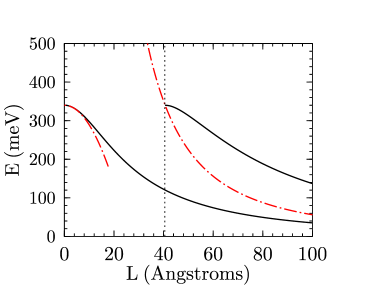
Figure 1: The energy levels dependence on the well’s width. The ground and the first excited levels (solid lines) are shown for the finite quantum well. Dot-dashed lines show the ground state level for the infinite well of the same width and $\delta$-functional potential (18) with $\alpha=UL$. A vertical dashed line is the well’s width at which the second level in the finite quantum well appears. It shows the range of applicability of the $\delta$-functional potential with the effective strength $\alpha=UL_{\textrm{eff}}$. Parameters are taken for a conduction band electron in an Al_0.3Ga_0.7As/GaAs quantum well (see below in a text).

For the $\delta$-functional potential it is more convenient to count energies from the barrier band edge rather than from the bottom of the well. In terms of the total Hamiltonian (1) it means that the energy band gap constant is the barrier’s energy band gap: $E_{g}^{\textrm{bar}}=E_{g}^{\textrm{well}}+U_{e}+U_{h}$. The energy and wave function of a single localized state are well-known:

$$E_{e,h}=-\frac{\kappa_{e,h}^{2}}{2m_{e,h}},\qquad\chi_{e,h}(z)=\sqrt{\kappa_{e,h}}\exp(-\kappa_{e,h}|z|).$$ (20)

Parameters $\kappa_{e,h}=\alpha_{e,h}m_{e,h}$ determine the localization of wave functions of an electron and a hole, respectively. It is worth noting that even for a very shallow quantum well, the localization length ($\sim 1/\kappa$) might be much less than the effective Bohr radius. In this case, we can expect a quasi-two dimensional behavior for the exciton, justifying the approximation for the mean field function in form (6). In the case of the AlGaAs/GaAs quantum wells, the electron (hole) localization length is smaller than Bohr’s radius up to $L\approx 5\AA$.

With the help of the wave functions (20), it is possible to obtain the analytical expression for the effective exciton potential $\overline{V}^{(0)}_{r}(r)$. The details of these calculations are given in Appendix A. The result is

$$\overline{V}^{(0)}_{r}(r;\kappa_{e},\kappa_{h})=-\frac{2\kappa_{e}\kappa_{h}}{\kappa_{h}^{2}-\kappa_{e}^{2}}\left[\kappa_{h}T(\kappa_{e}r)-\kappa_{e}T(\kappa_{h}r)\right],$$ (21)

where the function $T(\kappa r)$ is a combination of zeroth-order Struve and Neuman functions:Abramowitz and Stegun (1965)

$$T(\kappa r)=\frac{\pi}{2}\left[\textbf{H}_{0}(2\kappa r)-\textrm{Y}_{0}(2\kappa r)\right].$$ (22)

The behavior of the potential (21) is shown in Figure 2.

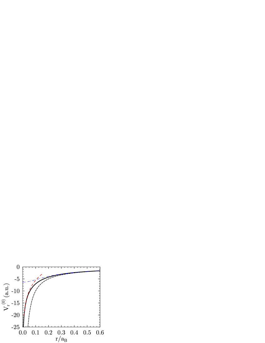
Figure 2: An effective self-consistent potential $\overline{V}^{(0)}_{r}$ profile for a two-dimensional exciton. The solid thick line represents Eq. (21). The dashed-dotted line is the approximation $(r^{2}+d^{2})^{-1/2}$, the dashed line is the logarithmic regime Eq. (25) for small $r$, the dotted line represents $1/r$ behavior. All data are for $d/a_{B}=0.16$ corresponding to $L=20\AA$ finite quantum well in AlGaAs/GaAs materials.

The behavior of the potential (21) has two regimes that are determined by the parameter

$$d=\sqrt{\frac{1}{2}\left(\frac{1}{\kappa_{e}^{2}}+\frac{1}{\kappa_{h}^{2}}\right)}.$$ (23)

This parameter has the meaning of an average electron-hole separation in the $z$ direction. For large distances, potential (21) has asymptotic behavior

$$V_{\textrm{asym}}(r)\approx-\frac{1}{\sqrt{r^{2}+d^{2}}},\qquad r\gtrsim d.$$ (24)

At small distances, the attraction becomes stronger. It has logarithmic behavior:

$$V_{\textrm{sm}}(r)\approx\frac{1}{d}\left[\ln(r/d)-1+\gamma\right],\qquad r\lesssim d,$$ (25)

where $\gamma=0.5772$.

Thus, the effective electron-hole interaction for the exciton in the quantum well starts from the true logarithmic Coulomb potential of a point charge in two dimensions that smoothly transforms at distances $r\sim d$ to the screening potential (24) with three-dimensional Coulomb tails. For the strong confinement $d\ll 1$ we can approximate $V_{\textrm{eff}}(r)$ by Eq. (24) for all distances and take into account the logarithmic part on the next step as a perturbation.

It is interesting to note that potential (24) can be obtained without the self-consistent procedure from the following simple intuitive consideration. At the first step, lets us neglect the electron-hole interaction in Hamiltonian (1). Then, we can solve the one-dimensional one-particle Schrödinger equations in the quantum well, and find the average square of the distance between the electron and the hole as

$$d^{2}=\langle\chi_{e}(z_{e})\chi_{h}(z_{h})|(z_{e}-z_{h})^{2}|\chi_{e}(z_{e})\chi_{h}(z_{h})\rangle.$$ (26)

This yields the same result as Eq. (23). The next step in the approximation of the Hamiltonian (1) is to include the Coulomb attraction term, where $(z_{e}-z_{h})^{2}$ is substituted by its average value $\langle\ (z_{e}-z_{h})^{2}\ \rangle$.

IV Numerical results: comparison with standard variational approach

The Schrödinger equation for a radial wave function in the central field (21) does not have an analytical solution. To obtain an approximate analytical expression for the exciton binding energy we will use the following procedure.

First of all, let us stress again that despite the fact that we consider a shallow quantum well with one single particle eigenvalue inside, the strong confinement persists up to very small widths. The parameter $d$ is a good indicator of such confinement. For example, in Table 1 the data are presented for Al_0.3Ga_0.7As-GaAs materials. We can see that for the well’s width of $10\AA$ this parameter is about one quarter of the three-dimensional Bohr radius and even smaller for larger quantum wells. For the case of strong confinement, $d\ll 1$, the effective potential (21) can be represented by Eq. (24) almost everywhere. Therefore, at the first step, it is reasonable to substitute the potential (21) by its asymptotic form (24) for all distances.

Appendix B yields the details of numerical calculations and analytical limits for the ground state in the potential. Although the Schrödinger equation with the potential (24) also does not have an analytical solution, we discovered that the ground state energy, obtained by the variational method for the single parameter trial function

$$\varphi_{trial}=\frac{2\exp(d/\lambda)}{\sqrt{\lambda(\lambda+2d)}}\exp(-\sqrt{r^{2}+d^{2}}/\lambda),$$ (27)

coincides with the exact one with excellent accuracy. To check this, we performed a precise numerical integration of the Schrödinger equation based on Pruefer transformation and a shooting method. The difference in the ground state energies for the whole range of the parameter $d$ was less than $0.01\%$, or $\sim 10^{-3}$ meV! Such an agreement can be explained by the fact that trial function (27) has a correct analytical behavior for both small and large distances, $r$.

The expression for the ground state energy obtained for the trial function (27) is given by

$$E_{X}^{(0)}(\lambda)=-\frac{2}{\lambda}\frac{1}{1+2d/\lambda}+\frac{1}{\lambda^{2}}\left[1-\frac{(2d/\lambda)^{2}E_{1}(1,2d/\lambda)\exp(2d/\lambda)}{1+2d/\lambda}\right],$$ (28)

where $\textrm{E}_{1}(x)$ is the exponential integral.Abramowitz and Stegun (1965) The variational parameter $\lambda$ changes from $1.1$ to $0.74$ when the average electron-hole distance $d$ varies from 0.11 to 0.48. The latter corresponds to the quantum well widths range from $40\AA$ to $5\AA$ for the AlGaAs/GaAs structures. The behavior of the parameter $\lambda$ as a function of $d$ is shown in the insert of Fig. 3. At small $d$ it has the following form:

$$\lambda\approx\frac{1}{2}+4d+\frac{d^{2}}{\lambda^{2}}\left[4\ln\left(\frac{2d}{\lambda}\right)-12\lambda+4\gamma+1\right].$$ (29)

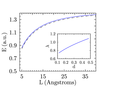
Figure 3: The exciton binding energies in the shallow quantum well for different well widths $L$. The solid line represents the two-dimensional exciton ground state, Eqs. (28) and (30) in the effective potential. The dotted-dashed line is the exciton binding energy obtained with the help of the variational method with the trial function (32). The insert shows the dependence of the parameter $\lambda$ on the average electron-hole separation $d$ in Eq.  (28). Both parameters are expressed in Bohr radius units and are presented for the same range of quantum well widths.

At small distances the effective potential (21) differs from Eq. (24). The correction to the energy due to this difference can be taken into account with the help of perturbation theory:

$$E_{X}^{(1)} = \langle\varphi_{trial}|\Delta V|\varphi_{trial}\rangle\approx\int_{0}^{d}\varphi_{trial}^{2}(r)\left[\frac{1}{d}\ln(r/d)\right]r\,dr$$ (30)

$$= -\frac{2d}{\lambda^{2}}\left[\frac{1}{2}-0.557\frac{2d}{\lambda}+0.563\left(\frac{2d}{\lambda}\right)^{2}+\cdots\right].$$ (31)

The last column of the Table 1 represents the final sum $E_{X}^{sc}=E_{X}^{(0)}+E_{X}^{(1)}$ for the exciton binding energy obtained by the self-consistent approach.

Table 1: Effective parameters of single quantum well potentials, electron, hole and exciton binding energies for different quantum well widths, $L$. Single particle electron and hole energies, $E_{e,h}^{(0)}$, are the initial step in the self-consistent field iterations [see Eq. (13)] when effective Coulomb terms $\overline{V}_{e,h}$ are omitted. These energies determine the strength parameters, $L_{\textrm{eff}}^{e,h}$, for corresponding $\delta$-potentials and the average distance, $d$, between an electron and a hole [Eq. (23)]. Energies $E_{X}^{(1),(2),(3)}$ are the exciton binding energies obtained by variational method with the trial functions given by Eqs. (32),(33), and (34), respectively. The last column shows the energy $E_{X}^{sc}=E_{X}^{(0)}+E_{X}^{(1)}$ [see Eqs. (28),(30)] obtained by the first iteration of the self-consistent approach. The calculations are based on the following physical constants:Miller et al. (1985) $m_{e}^{*}=0.067m_{0}$, $m_{h}^{*}=0.45m_{0}$, $U_{e}=340$ meV, $U_{h}=70$ meV, $\epsilon=13.8$. For these parameters the effective Bohr radius is $a_{B}=125\AA$ and the energy atomic unit is equal to 8.33 meV.

$L\ (\AA)$	$L_{\textrm{eff}}^{e}\ (\AA)$	$L_{\textrm{eff}}^{h}\ (\AA)$	$d(a.u.)$	$-E_{e}^{(0)}$ (a.u.)	$-E_{h}^{(0)}$ (a.u.)	$-E_{X}^{(1)}$ (a.u.)	$-E_{X}^{(2)}$ (a.u.)	$-E_{X}^{(3)}$ (a.u.)	$-E_{X}^{\textrm{sc}}$ (a.u.)
10	9.15	8.89	0.257	5.11	1.37	1.0799	1.0975	1.1041	1.0948
20	15.16	14.12	0.158	14.02	3.46	1.2617	1.2779	1.2843	1.2754
30	18.63	16.88	0.130	21.18	4.95	1.3314	1.3467	1.3527	1.3443
40	20.70	18.43	0.118	26.12	5.90	1.3655	1.3802	1.3855	1.3779

To check the accuracy of our method we compared the results of the self-consistent approach with the results of the standard variational method for three different trial functions. These trial functions have the following forms:

$$\psi^{(1)}(z_{e},z_{h},r;\lambda) = \sqrt{\kappa_{e}\kappa_{h}}\exp(-\kappa_{e}|z_{e}|-\kappa_{h}|z_{h}|)\exp(-r/\lambda),$$ (32)

$$\psi^{(2)}(z_{e},z_{h},r;\lambda,\beta) = \sqrt{\kappa_{e}\kappa_{h}}\exp(-\kappa_{e}|z_{e}|-\kappa_{h}|z_{h}|)\exp(-\sqrt{r^{2}+\beta^{2}}/\lambda),$$ (33)

$$\psi^{(3)}(z_{e},z_{h},r;\lambda,\beta) = \sqrt{\kappa_{e}\kappa_{h}}\exp(-\kappa_{e}|z_{e}|-\kappa_{h}|z_{h}|)\exp(-\sqrt{r^{2}+\beta^{2}(z_{e}-z_{h})^{2}}/\lambda),$$ (34)

The first two functions are separable, while the third one is non-separable. The first wave function has one variational parameter $\lambda$, and two others have two variational parameters $\lambda$ and $\beta$.

The details of variational calculations are given in Appendix C. Our results and their comparison with data obtained by the standard variational procedure are presented in Table 1.

We can see that the single parameter separable trial function, $\psi^{(1)}(z_{e},z_{h},r;\lambda)$, gives higher binding energy with maximal relative difference of $1.3\%$. The non-separable trial functions have slightly lower binding energies than the first iteration of the self-consistent approach. The maximum relative difference between the self-consistent binding energy $E_{X}^{sc}$ and the binding energy $E_{X}^{(2)}$ is $0.24\%$ (for AlGaAs/GaAs structures it corresponds to a difference of $0.02$ meV). For $E_{X}^{(3)}$ it is $0.84\%$ ($0.07$ meV). These results demonstrate that even the first iteration of our approach gives an excellent agreement with the variational results. Subsequent iterations further decrease the ground state energy. Preliminary research on the convergence of the self-consistent approach shows that the next iteration gives the value of the binding energy lower than the variational calculations with trial functions (33) and (34). These results will be published elsewhere. However, in the particular case considered here the difference by $0.07$ meV between more complicated variational approach and the results presented here is already much smaller than the accuracy of, for instance, optical absorption experimentsVoliotis et al. (1995), which is of the order of $2$ meV. From this point of view the discrepancy between the two methods is negligible. At the same time, our approach is about $100$ times faster than the variational method even with the simple enough trial function, Eq. (33). It also helps to avoid a numerically difficult task of finding minima of several non-polynomial functions. The additional physical information about the effective potential allows one to find one of the variational parameters of function (33) without minimization.

V Conclusions

We introduce a self-consistent approach for calculations of the exciton binding energy in a quantum well. For the case of strong confinement, the self-consistent Hamiltonian is separable and consists of three parts: one-dimensional Hamiltonians for electron and hole confined motions across the quantum well, and the Hamiltonian, which describes the motion of a two-dimensional exciton in the effective central field potential. This effective potential is a result of averaging over $z$ coordinates of the Coulomb interaction and the quantum well potential. As a function of distance the effective potential has two different regimes of behavior which are determined by the average distance between electron and hole inside the quantum well, $d$. For small distances, $r\lesssim d$, the effective potential has a logarithmic form of a Coulomb potential of a point charge in two dimensions. At a distance $r\sim d$ this behavior crosses over to the three-dimensional Coulomb screened potential, $-1/\sqrt{r^{2}+d^{2}}$. For the case of the shallow quantum well, analytical formulae, Eqs. (28) and (30), for the exciton binding energy are obtained. Even though the use of these formulae requires computational time which is by orders of magnitude smaller than that of standard variational calculations, the results obtained by both methods are in an excellent agreement. The differences between the exciton binding energies in two approaches are generally smaller than $1\%$. For AlGaAs/GaAs structures it corresponds to differences smaller than $0.1$ meV, i.e. smaller than correctionsAndreani and Pasquarello (1990) due to non-parabolicity of the bulk conduction band or dielectric constant and effective mass mismatches. One can expect that the developed method can lay the foundation for models that incorporate these important effects as well as take into account an influence of the external electric field.

All results discussed above are obtained for the first successive iteration. Obviously, the next iterations will lower the ground state energy even more. For example, the next step is the substitution of the wave function (27) into Eq. (11), which is approximately equivalent to the appearance of additional oscillatory potentials in Eqs. (8) and (9):

$$\overline{V}_{e,h}(z_{e,h})\approx-\overline{(r^{2}+d^{2})^{-1/2}}+\frac{\overline{(r^{2}+d^{2})^{-3/2}}}{2}\left(z_{e,h}^{2}-\overline{z^{2}_{e,h}}\right).$$ (35)

These potentials will slightly change the single-particle energies and will localize the tails of the eigenfunctions of the electron and the hole ground states. The latter will be manifested in a decrease of the average electron-hole distance $d$, and, therefore, will lower the exciton binding energy in the next successive iteration of Eq. (7).

In derivation of our results we used three different approximations. They are: (i) the self-consistent approach itself, (ii) the use of the factorized form of the wave function, (iii) and the use of the delta-functional potential for a shallow quantum well. The self-consistent approach is broader than the standard variational method since we do not have to specify a particular functional dependence for a trial function. Instead, we just suggest that the trial function consists of some combination of unknown functions. The factorized form is the simplest form for such a combination but it is not required by our method. The method can be applied to other physical models where different types of trial functions would be more natural. For example, for a wide double quantum well, the better choice of the trial function of the ground state is a superposition of two factorized single-well functions. It will result in a system of coupled equations similar (but more complicated) to Eqs. (7)–(9). This approach can also be straightforwardly expanded to include other effects, which were neglected in this paper. For instance, in order to take into account the dielectric mismatch,Andreani and Pasquarello (1990); de Leon and Laikhtman (2000); Gerlach et al. (1998) we would need to correct the expression for the effective potentials, Eq. (10) and Eq. (11), including effects of image charges into the respective integrals. The valence band degeneracy and anisotropy can be included by introducing a four component trial function, for which the self-consistent equations will have the similar form as Eqs. (7)–(9), but they should be understood as matrix equations.

Turning to the particular factorization used in our problem, it is obvious that the more strongly the exciton is localized in the $z$-direction (size of wave function in $z$-direction compared to the three-dimensional Bohr radius) the better our approximation works. If we consider the case of Al_0.3Ga_0.7As-GaAs quantum well, it means that our method will work for any quantum well with a width less that $100\ \AA$, but the best convergence will happen somewhere around $30-50\ \AA$. Correspondingly, the factorized form of the trial function for the self-consistent method is applicable for any structure (e.g., asymmetric quantum well or quantum well in electric field), if a wave function localized in $z$-direction has such an extension. In a similar matter the self-consistent approach can be applied to the lower dimension systems such as quantum wires and quantum dots. Moreover, preliminary consideration showed that the problem of divergency of the exciton ground state in a one-dimensional Coulomb potential, which arises in other approaches to quantum wires, in this method does not appear at all.

The $\delta$-functional potential is a good approximation if a one-dimensional quantum well has only one level (is shallow). For a typical case of Al_0.3Ga_0.7As-GaAs quantum well, it gives an applicability range of $L<40\ \AA$. The approximation of the $\delta$-functional potential gives simple single-particle wave functions that significantly simplify calculations of the effective potentials in Eqs. (10) and (11). If asymmetric quantum well or double quantum wells, or quantum well in electric field are shallow, the delta-functional approach will be applicable to such models. An asymmetric quantum well can be modelled by a quantum barrier and the $\delta$-functional potential ($\delta(z)\rightarrow\delta(z)[1+A\theta(z)]$, where $\theta$ is the step function). An advantage of using the $\delta$-functional potential is especially clear in the case of the quantum confined Stark effect for a shallow quantum well, where it allows one to obtain additional results related to the field-induced resonance widths for a single-particle as well as for the exciton quasi-bound states. These results will be published elsewhere.

Appendix A Effective potential for 2D exciton

The effective field for quasi 2D exciton is given by the integral

$$V_{\textrm{eff}}(r)=-\int_{-\infty}^{\infty}dz_{e}\int_{-\infty}^{\infty}dz_{h}\frac{\left|\chi_{e}(z_{e})\right|^{2}\left|\chi_{h}(z_{h})\right|^{2}}{\sqrt{r^{2}+(z_{e}-z_{h})^{2}}}.$$ (36)

For a shallow quantum well approximated by the $\delta$-function potential it gives

$$V_{\textrm{eff}}(r)=-\int_{0}^{\infty}dz_{1}\int_{0}^{\infty}dz_{2}e^{-2\kappa_{1}z_{1}}e^{-2\kappa_{2}z_{2}}\left[\frac{2\kappa_{1}\kappa_{2}}{\sqrt{r^{2}+(z_{1}-z_{2})^{2}}}+\frac{2\kappa_{1}\kappa_{2}}{\sqrt{r^{2}+(z_{1}+z_{2})^{2}}}\right]=V_{1}+V_{2}.$$ (37)

After making the coordinate transformation $\xi=z_{1}-z_{2},\ \eta=z_{1}+z_{2}$ and taking into account that

$$\int_{0}^{\infty}dz_{1}\int_{0}^{\infty}dz_{2}f(\xi,\eta)=\frac{1}{2}\int_{0}^{\infty}d\eta\int_{-\eta}^{\eta}d\xi f(\xi,\eta)=\frac{1}{2}\int_{0}^{\infty}d\xi\int_{\xi}^{\infty}d\eta\left[f(-\xi,\eta)+f(\xi,\eta)\right],$$ (38)

the first integration in these two interated integrals becomes trivial and the second integration can be expressed through the function

$$T(\kappa r)=\int_{0}^{\infty}\frac{\exp(-2\kappa t)dt}{\sqrt{r^{2}+t^{2}}}=\frac{\pi}{2}\left[\textbf{H}_{0}(2\kappa r)-\textrm{Y}_{0}(2\kappa r)\right],$$ (39)

where $\textbf{H}_{0}$ is the zeroth-order Struve function and $\textrm{Y}_{0}$ is the zero-order Neumann or Bessel function of the second kind.Abramowitz and Stegun (1965) Then potentials $V_{1}$ and $V_{2}$ can be expressed as

$$V_{1,2}=-\frac{\kappa_{1}\kappa_{2}}{\kappa_{1}\pm\kappa_{2}}\left[T(\kappa_{2}r)\pm T(\kappa_{1}r)\right],$$ (40)

and the final result yields Eq. (21)

$$V_{\textrm{eff}}(r;\kappa_{1},\kappa_{2})=-\frac{2\kappa_{1}\kappa_{2}}{\kappa_{2}^{2}-\kappa_{1}^{2}}\left[\kappa_{2}T(\kappa_{1}r)-\kappa_{1}T(\kappa_{2}r)\right].$$ (41)

In the case when $\kappa_{1}=\kappa_{2}\equiv\kappa$ this expression is reduced to

$$V_{\textrm{eff}}(r;\kappa)=-\kappa\left[T(\kappa r)-\kappa T^{\prime}(\kappa r)\right],$$ (42)

where

$$T^{\prime}(\kappa r)=\frac{\partial T}{\partial\kappa}=2r\left[\frac{\pi}{2}\textrm{Y}_{1}(2\kappa r)-\frac{\pi}{2}\textbf{H}_{1}(2\kappa r)+1\right].$$ (43)

Appendix B Eigenvalues and eigenfunctions in $2D$ central potentials

The Schrödinger equation for a radial wave function in a central field is

$$\left[\frac{\partial^{2}}{\partial r^{2}}+\frac{1}{r}\frac{\partial}{\partial r}-\frac{m^{2}}{r^{2}}-2U(r)+2E\right]\varphi(r)=0.$$ (44)

For the Coulomb potential, $U(r)=-Z/r$, the ground state is well-known:

$$E_{1}=-2Z^{2},\quad\varphi_{1}(r)=\frac{4Z}{\sqrt{2\pi}}e^{-2rZ}.$$ (45)

Let us consider now the potentialPonomarev et al. (1999)

$$U(r)=-1/\sqrt{r^{2}+d^{2}}.$$ (46)

The ground state energy and the eigenfunction for Eq. (44) with the potential (46) are presented in Fig. 4.

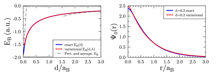
Figure 4: (a) The ground state energy for the potential $-(r^{2}+d^{2})^{-1/2}$, Eq. (46), as functions of the parameter $d$. Solid line, representing numerical results, and dashed line, obtained by the use of variational formula (48), are practically indistinguishable. The dot-dashed lines correspond to perturbation theory for small $d$ and an asymptotic oscillatory energy $-d^{-1}+d^{-3/2}$ for $d\gg 1$. (b) The ground state wave function for $d=0.2$. The numerical results are shown by the solid line. The dashed line corresponds to Eq. (47) for normalized trial function.

It turns out that the numerical results are in an extremely good agreement ($\sim 0.01\%$) with the results of variational method for the trial function

$$\varphi_{trial}=\frac{2\exp(d/\lambda)}{\sqrt{\lambda(\lambda+2d)}}\exp(-\sqrt{r^{2}+d^{2}}/\lambda),$$ (47)

where $\lambda$ is the only variational parameter. The corresponding value for ground state energy is obtained from minimization of the functional

$$E_{X}(\lambda)=-\frac{2}{\lambda}\frac{1}{1+2d/\lambda}+\frac{1}{\lambda^{2}}\left[1-\frac{(2d/\lambda)^{2}E_{1}(1,2d/\lambda)\exp(2d/\lambda)}{1+2d/\lambda}\right].$$ (48)

Such a good agreement can be explained by the fact that the trial function (47) has correct asymptotic behavior in both limits of small and large $r$.

Far away from the “atomic residue” $U(r)\sim-1/r$, the wave function for the $s$-state obeys the Schrödinger equation

$$-\frac{\Delta}{2}\varphi-\frac{1}{r}\varphi=-\frac{\alpha^{2}}{2}\varphi$$

with the solution

$$\varphi(r)=A_{\alpha}r^{1/\alpha-1/2}e^{-\alpha r},$$ (49)

where terms of the order of $\varphi/r^{2}$ are neglected. Here $A_{\alpha}$ and $\alpha$ are atomic parameters. Their magnitudes are determined by the behavior of an electron inside the “atom”.

Simple analytical estimates for the cases of small and large $d$ for ground state energy and the asymptotic coefficient $A_{\alpha}$ can be made. When $d\ll 1$ the potential is only slightly different from the Coulomb potential and the contribution to the energy can be obtained using perturbation theory:

$$E_{X}=-2+\langle 0|V|0\rangle\approx-2+16d\left(1+2d\ln(2d)\right).$$ (50)

Note, that due to the big factor in front of $d$ in Eq. (50), the convergence radius for the perturbation series is small enough.

Assuming that the asymptotic form (49) of the wave function is valid for all values of $r$, we obtain the following simple estimate for $A_{\alpha}$

$$2\pi A_{\alpha}^{2}\int_{0}^{\infty}r^{2/\alpha}\exp(-2\alpha r)\,dr=1\Rightarrow A_{\alpha}=\frac{2^{1/\alpha-1/2}\alpha^{1/\alpha+1}}{\sqrt{\pi\Gamma(2/\alpha)}}.$$ (51)

In the opposite case, when $d\gg 1$ the solution has to be close to the oscillatory one

$$E_{X}=-\frac{1}{d}+\frac{1}{d^{3/2}}(n+1),$$ (52)

where $n=0,1,2...$. The main contribution to the normalization comes from the Gaussian part of the wave function because the contribution of the Coulomb tails is negligible. One obtains for the state with $n=0$

$$\varphi(r)\approx\varphi_{osc}(r)=\sqrt{\frac{\omega}{\pi}}\exp\left(-\omega r^{2}/2\right),$$ (53)

where $\omega=1/d^{3/2}$. Then,

$$A_{\alpha}=\frac{1}{\sqrt{\pi}d^{3/4}}.$$ (54)

Appendix C Variational method for excitons in $\delta$-function quantum wells

Following standard procedures the envelope variational exciton wave function in a quantum well can be presented as a product of three terms,

$$\Psi(z_{e},z_{h},r;\lambda_{i})=\chi_{e}(z_{e})\chi_{h}(z_{h})\phi(r,z_{e},z_{h};\lambda_{i}),$$ (55)

where $\lambda_{i}$ is the set of variational parameters and $\phi$ is the variational wave function which minimizes the total energy of the Hamiltonian (1). Two other factors $\chi_{e,h}(z_{e,h})$ are simply normalized eigenfunctions of the one-particle electron or hole Hamiltonians of the quantum well:

$$E_{e,h}\chi_{e,h}(z_{e,h}) = \left[-\frac{1}{2m_{e,h}}\frac{\partial^{2}}{\partial z_{e,h}^{2}}-\alpha_{e,h}\delta(z_{e,h})\right]\chi_{e,h}(z_{e,h}),$$

$$\chi_{e,h}(z_{e,h}) = \sqrt{\kappa_{e,h}}\exp(-\kappa_{e,h}|z_{e,h}|),$$

$$\kappa_{e,h} = m_{e,h}\alpha_{e,h},\qquad E_{e,h}=\kappa_{e,h}^{2}/2m_{e,h}.$$ (56)

To obtain more confident results we made calculations with three different trial functions $\psi$:

$$\psi^{(1)}(r;\lambda) = \exp(-r/\lambda),$$ (57)

$$\psi^{(2)}(r;\lambda,\beta) = \exp(-\sqrt{r^{2}+\beta^{2}}/\lambda),$$ (58)

$$\psi^{(3)}(r,|z_{e}-z_{h}|;\lambda,\beta) = \exp(-\sqrt{r^{2}+\beta^{2}(z_{e}-z_{h})^{2}}/\lambda),$$ (59)

The first two functions are independent of $z$ coordinates, while the third one is non-separable with respect to $z$. The first wave function has one variational parameter $\lambda$, and two others have two variational parameters $\lambda$ and $\beta$.

The total exciton energy is the minimum of the functional

$$E=\frac{\langle\Psi|\hat{H}|\Psi\rangle}{\langle\Psi|\Psi\rangle}.$$ (60)

For the first two trial functions, which are independent of $z$, the functional (60) can be further simplified. In this case, the energy can be presented as

$$E=E_{e}+E_{h}+\overline{K}/N+\overline{V}/N,$$ (61)

where

$$N = \langle\Psi|\Psi\rangle,\equiv\langle\psi(r)|\psi(r)\rangle\,$$ (62)

$$\overline{K} = \langle\psi(r)|\hat{K_{r}}|\psi(r)\rangle\ \equiv\frac{1}{2}\int\left(\nabla\psi\right)^{2}dA,$$ (63)

$$\overline{V} = -\langle\Psi|\frac{1}{\sqrt{r^{2}+(z_{e}-z_{h})^{2}}}|\Psi\rangle\ \equiv\int\left(V_{\textrm{eff}}(r)|\psi(r)|^{2}\right)dA,$$ (64)

Calculations for the trial function $\psi^{(2)}$ yield

$$N^{(2)} = \frac{\exp(-2\beta/\lambda)\lambda(\lambda+2\beta)}{4},$$

$$\overline{K}^{(2)} = \frac{\exp(-2\beta/\lambda)}{8}\left[1+\frac{2\beta}{\lambda}-\left(\frac{2\beta}{\lambda}\right)^{2}\textrm{E}_{1}(2\beta/\lambda)\exp(2\beta/\lambda)\right],$$

$$\overline{V}^{(2)} = -\frac{2\kappa_{1}\kappa_{2}}{\kappa_{2}^{2}-\kappa_{1}^{2}}\left[\kappa_{2}V(\kappa_{1},\lambda,\beta)-\kappa_{1}V(\kappa_{2},\lambda,\beta)\right],$$ (65)

where $\textrm{E}_{1}(x)$ is the exponential integralAbramowitz and Stegun (1965) and

$$V(\kappa,\lambda,\beta)=\int_{0}^{\pi/2}\cos(\phi)\;d\phi\int_{0}^{\infty}\exp(-2\kappa R\sin(\phi)-2\sqrt{R^{2}\cos^{2}(\phi)+\beta^{2}}/\lambda)R\;dR.$$ (66)

For the first trial function $\psi^{(1)}(r;\lambda)\equiv\psi^{(2)}(r;\lambda,0)$ all integrals have analytical expressions:

$$N^{(1)} = \frac{\lambda^{2}}{4},$$

$$\overline{K}^{(1)} = \frac{1}{8},$$

$$V(\kappa,\lambda,0) = \frac{\lambda^{2}}{4}\frac{1}{1+\lambda^{2}\kappa^{2}}\left[\lambda\kappa-1+\frac{1}{\sqrt{1+\lambda^{2}\kappa^{2}}}\ln\left(\frac{1}{\lambda\kappa}\frac{\sqrt{1+\lambda^{2}\kappa^{2}}+1}{\sqrt{1+\lambda^{2}\kappa^{2}}-\lambda\kappa}\right)\right].$$ (67)

Integrals for the non-separable trial function $\psi^{(3)}$ can be numerically estimated following the procedure described in Ref. Harrison et al., 1996; Harrison, 1999

References

- Harrison (1999) P. Harrison, ed., Quantum wells, wires, and dots: theoretical and computational physics (John Wiley and Sons, Chichester, 1999).
- Burstein and Weisbuch (1995) E. Burstein and C. Weisbuch, eds., Confined Electrons and Photons: New Physics and Applications (Plenum Press, New York, 1995).
- Mendez and von Klitzing (1989) E. E. Mendez and K. von Klitzing, eds., Physics and Applications of Quantum Wells and Superlattices (Plenum Press, New York, 1989).
- Nolte (1999) D. D. Nolte, Journal of Applied Physics 85, 6259 (1999).
- Miller et al. (1981) R. C. Miller, D. A. Kleinman, W. T. Tsang, and A. C. Gossard, Phys. Rev. B 24, 1134 (1981).
- Bastard et al. (1982) G. Bastard, E. E. Mendez, L. L. Chang, and L. Esaki, Phys. Rev. B 26, 1974 (1982).
- Greene et al. (1984) R. L. Greene, K. K. Bajaj, and D. E. Phelps, Phys. Rev. B 29, 1807 (1984).
- Efros (1986) A. L. Efros, Sov. Phys. Semicond. 20, 808 (1986).
- Andreani and Pasquarello (1990) L. C. Andreani and A. Pasquarello, Phys. Rev. B 42, 8928 (1990).
- Gerlach et al. (1998) B. Gerlach, J. Wusthoff, M. O. Dzero, and M. A. Smondyrev, Phys. Rev. B 58, 10568 (1998).
- Iotti and Andreani (1997) R. C. Iotti and L. C. Andreani, Phys. Rev. B 56, 3922 (1997).
- Kossut et al. (1997) J. Kossut, J. K. Furdyna, and M. Dobrowolska, Phys. Rev. B 56, 9775 (1997).
- Harrison et al. (1996) P. Harrison, T. Piorek, W. E. Hagston, and T. Stirner, Superlatt. Microstruct. 20, 45 (1996).
- de Leon and Laikhtman (2000) S. de Leon and B. Laikhtman, Phys. Rev. B 61, 2874 (2000).
- Ekenberg and Altarelli (1987) U. Ekenberg and M. Altarelli, Phys. Rev. B 35, 7585 (1987).
- Chang et al. (1988) S. K. Chang, A. V. Nurmikko, J. W. Wu, L. A. Kolodziejski, and R. L. Gunshor, Phys. Rev. B 37, 1191 (1988).
- Warnock et al. (1993) J. Warnock, B. T. Jonker, A. Petrou, W. C. Chou, and X. Liu, Phys. Rev. B 48, 17321 (1993).
- Piorek et al. (1995) T. Piorek, P. Harrison, , and W. E. Hagston, Phys. Rev. B 52, 14111 (1995).
- Voliotis et al. (1995) V. Voliotis, R. Grousson, P. Lavallard, and R. Planel, Phys. Rev. B 52, 10725 (1995).
- Stahl and Balslev (1987) A. Stahl and I. Balslev, Electrodynamics of the Semiconductor Band Edge (Springer, Berlin, 1987).
- Balslev et al. (1989) I. Balslev, R. Zimmermann, and A. Stahl, Phys. Rev. B 40, 4095 (1989).
- Merbach et al. (1998) D. Merbach, E. Schöll, W. Ebeling, P. Michler, and J. Gutowski, Phys. Rev. B 58, 10709 (1998).
- Castella and Wilkins (1998) H. Castella and J. W. Wilkins, Phys. Rev. B 58, 16186 (1998).
- Miller et al. (1985) D. A. B. Miller, D. S. Chemla, T. C. Damen, A. C. Gossard, W. Wiegmann, T. H. Wood, and C. A. Burrus, Phys. Rev. B 32, 1043 (1985).
- Abramowitz and Stegun (1965) M. Abramowitz and I. A. Stegun, eds., Handbook of Mathematical Functions (Dover, New York, 1965).
- Ponomarev et al. (1999) I. V. Ponomarev, V. V. Flambaum, and A. L. Efros, Phys. Rev. B 60, 5485 (1999).