Solution of the local field equations for self-generated glasses

Abstract

We present a self-consistent local approach to self generated glassiness which is based on the concept of the dynamical mean field theory to many body systems. Using a replica approach to self generated glassiness, we map the problem onto an effective local problem which can be solved exactly. Applying the approach to the Brazovskii-model, relevant to a large class of systems with frustrated micro-phase separation, we are able to solve the self-consistent local theory without using additional approximations. We demonstrate that a glassy state found earlier in this model is generic and does not arise from the use of perturbative approximations. In addition we demonstrate that the glassy state depends strongly on the strength of the frustrated phase separation in that model.

I Introduction

The familiar example of vitrification upon super-cooling molecular fluids provides proof that an effectively non-ergodic disordered state can be generated in a system without pre-existing quenched disorder. Such self-generated glassiness may be a more widespread possibility in the material world than is currently acknowledged.  Candidate solid state systems with extremely slow dynamics often have impurities remaining from their synthesis so there is always a suspicion that non-ergodicity comes from disorder.mang01 ; Millis96 ; Dagotto ; nmr01 ; nmr02 ; nmr03 ; nmr3b ; nmr04 ; msr01 ; msr02 ; msr03 While a rather successful microscopic theory of molecular glasses now exists based on the idea of an underlying random first order transitionKTW89a ; KTW89b ; KTW89c ; KTW89d , this theory, like all theories of liquid state phenomena, contains approximations that can only be checked a posteriori through their agreement with simulations or experiments. To deepen and widen our understanding of glassy dynamics beyond the molecular fluid example, it would be desirable to have a model which can be analyzed in a formally exact fashion using familiar tools of continuum field theory. Such a theory would also help clarifying which features of the current theory of structural glasses are robust and ”protected”TOE and which are fortuitously correct.

Both, the recent treatment of the thermodynamics of fragile glasses developed within a replica formulationMP991 and the closely related approach using density functional theory for super-cooled liquidsSSW85  suggest that the major aspects of glass formation  stem from the very strong local correlations of a dense super-cooled fluid. This is very different  from systems with critical dynamics close to second order phase transitions, where long wavelength fluctuations are paramount. One finds experimentally that dynamics on essentially all wavelengths slows to nearly the same extent as the glass transition is approached. This suggests that the search for an solvable limit of the glass problem should focus on the strong but local nonlinearities.

Major progress has recently been made in the theoretical understanding of strongly interacting systems with predominantly local correlations. Strongly correlated electron systems like Mott insulators or systems with strong electron-phonon interactions have been investigated with the dynamic mean field theorydmft1 ; dmft2 (DMFT). Originally, this approach was based on the assumption that all non-trivial correlations of a given system are strictly local (for the precise definition of a local theory, see below) and then allowed for a solution of such systems without further approximations. More recently several generalizations of the approach have been developed, which allow the inclusion of collective excitationsSi ; CK90 as well as short range correlations in so called cluster DMFT theoriescluster2 ; cluster3 ; cluster .

In this paper we will follow the main strategy of the dynamic mean field approach and apply it to the replica theory of self generated glassiness. This allows us to solve completely for the long time correlation function (Edwards-Anderson parameter) as well as the configurational entropy of a glass within a local theory. Even though the origin of glassiness is not quenched disorder, there is a similarity between our theory and the mean field theory of spin glasses which is also exact in the limit of a purely local approach. Solvable local limits like the Sherrington-Kirkpatrick model, turned out to be extremely fruitful for the investigation of more realistic models. To identify and solve such a local problem is therefore of general interest. Another appealing aspect of the approach developed here is that the recent generalizations of the DMFT to cluster systems offer a feasible way to develop a controlled series of approximations for candidate glassy systems that successively extend the range of local correlations taken into account.cluster2 ; cluster3 ; cluster . Clearly, before this becomes possible we have to set up and analyze the strictly local (i.e. mean field) theory. The solutions of the local field theories discussed in this paper rely on a self consistency condition that is uniformly applied to the replicated statistical mechanics problem. The droplet effects that give rise to the activated transitions in molecular fluids cannot be described by this uniform replica symmetry breaking ansatz. While the self consistent replica field theory is applicable to account for some geometric effects in finite dimensions the latter highly nonperturbative effects are absent, but are suppressed if the coordination number is high. We should also mention that related interesting approach to self-generated glassiness in a model in infinite dimensions (where the locality of the problem is exactly guaranteed) that was recently presented by Lopatin and Ioffe.Lopatin

We demonstrate that a uniformly frustrated system with competition of interactions on different length scales undergoes a glass transition once inhomogeneous fluctuations become strong enough if no ordered phase forms via nucleation. Specific calculations are carried out for the case of the Brazovskii modelBrazovskii , which describes systems with tendency towards micro-phase separation. Glassiness was shown to exist in this model in Refs.SW00, ; SWW00, . However, it remained unclear to what extent this is merely a consequence of an approximate solution using perturbation theory or is indeed the correct mean field behavior of this model.

In the next section we briefly summarize the replica approach to self generated glassiness, present the main idea of the dynamic mean field theory and solve the local theory for self generated glassiness in case of the Brazovskii model. We  summarize the results of this paper in Section III.

II Theory

II.1 The replica approach

In this paper we consider physical systems consisting of $\ L$-components (types of atoms or molecules) and with short ranged $3^{\mathrm{rd}}$, $4^{\mathrm{th}}$ and higher  order virial coefficients. No specific assumption is made with respect to the (possibly non local)  $2^{\mathrm{nd}}$ virial coefficient.  In terms of a density field $\rho_{l}\left(\mathbf{x}\right)=\sum_{i}\delta\left(\mathbf{x-X}_{i,l}\right)$ of particles of type $l=1,...,L$ ( $L=1$ in case of a one component system) we then have an effective energy:

$$H\left[\phi\right]=H_{0}\left[\phi\right]+\int d^{d}xV\left(\phi_{l}\left(\mathbf{x}\right)\right)$$ (1)

with

$$H_{0}=\int d^{d}xd^{d}x^{\prime}\sum_{ll^{\prime}}\phi_{l}\left(\mathbf{x}\right)G_{0ll^{\prime}}^{-1}\left(\mathbf{x},\mathbf{x}^{\prime}\right)\phi_{l^{\prime}}\left(\mathbf{x}^{\prime}\right).$$ (2)

where $\phi_{l}\left(\mathbf{x}\right)=\rho_{l}\left(\mathbf{x}\right)-\overline{\rho}_{l}$ is the deviation of the density from its average value. The key assumption made in Eqs.1 and 2 is the local character of $V\left(\phi\right)$ which includes the higher order virial coefficients. For example, Eq.1, might be a representation of the density functional used by Ramakrishnan and Youssoff with $G_{0ll^{\prime}}^{-1}\left(\mathbf{x},\mathbf{x}^{\prime}\right)=c_{ll^{\prime}}\left(\mathbf{x}-\mathbf{x}^{\prime}\right)$ the direct correlation function of the fluidHansen and

$$V\left(\phi\right)=\sum_{l}\left(\overline{\rho}_{l}+\phi_{l}\left(\mathbf{x}\right)\right)\left[\log\left(\overline{\rho}_{l}+\phi_{l}\left(\mathbf{x}\right)\right)-1\right]$$ (3)

the ideal gas free energy.

The partition function of the system is given by

$$Z_{\mathrm{eq}}=\int D\phi\exp\left(-H\left[\phi\right]/T\right)$$ (4)

and determines the equilibrium properties of the system. In a system with complex energy landscape where we expect that the system might undergo vitrification, the knowledge of the equilibrium partition function is not sufficient anymore.

A widely accepted viewKTW89a ; KTW89b is that a glassy system may be  considered to be trapped in local metastable states for very long time and can therefore not realize a considerable part of the entropy of the system,  called the configurational entropy $S_{\mathrm{c}}=\log\mathcal{N}_{\mathrm{ms}}$, where $\mathcal{N}_{\mathrm{ms}}$ is the number of metastable states. If $\mathcal{N}_{\mathrm{ms}}$ is exponentially large with respect to the size of the system, $S_{\mathrm{c}}$ becomes extensive and ordinary equilibrium thermodynamics fails. There are several theoretical approaches which offer a solution to this breakdown of equilibrium many body theory. On the one hand one can solve for the time evolution of correlation and response functions, an approach which explicitly reflects the dynamic character of the glassy state. Mostly because of its technical simplicity, an alternative (but equivalent) approach is based on a replica theoryMon95 ; MP991 . Even though this approach does not allow one to calculate the complete time evolution, long time correlations as well as stationary response functions can be determined which are in agreement with the explicit dynamic theory. We will use the replica approach because of its relative simplicity.

The central quantity of the replica theory to self generated glassiness is the replicated partition functionMon95 ; MP991

$$Z\left(m\right)=\int D^{m}\phi e^{-\sum_{\alpha}^{m}H\left[\phi_{\alpha}\right]\ +g\int\frac{dx}{2m}\sum_{\alpha,\beta}^{m}\phi_{\alpha}\left(\mathbf{x}\right)\phi_{\beta}\left(\mathbf{x}\right)}.$$ (5)

$Z\left(m\right)$ must be analyzed in the limit $m\rightarrow 1$ and $g\rightarrow 0$ which is taken at the end of the calculation. One can interpret $Z\left(m\right)$ as the result of a quenched average over random field configurations with infinitesimal disorder strength $g$ and a distribution function which is determined by the partition function of the system itself. A similar approach (however for finite $g$) was proposed by Deam and EdwardsED75 in the theory of the vulcanization transition where the distribution of random cross-links of a polymer melt is also determined by the actual partition function of the polymer system itselfPaul .  Then, just as in the present approach, the number of replicas, $m$, is taken to the limit $m\rightarrow 1$, as opposed to the usual $m\rightarrow 0$ limit used for systems with averaging over ”white”  quenched disorder distributions. In the vulcanization problem, $g$ is related to the cross link density and, in distinction to the theory presented here, remains finite.  Physically, the analysis of $Z\left(m\right)$ addresses whether the system drives itself  ($m\rightarrow 1$)  into a glassy state if exposed to an infinitesimally weak randomness ($g\rightarrow 0$). It can be shownWSW02 that this approach is equivalent to the solution of the dynamic equations for the correlation and response functionCK93 of the system that takes aging and long term memory effects into account.

$F\left(m\right)=-\frac{T}{m}\log Z\left(m\right)$ determines the configurational entropy, $S_{\mathrm{c}}$, and the averaged free energy of systems trapped in metastable states, $\widetilde{F}$, viaMon95 ; MP991 ; SWW00

$$\widetilde{F} = \lim_{g\rightarrow 0}\left.\frac{\partial\left(mF\left(m\right)\right)}{\partial m}\right|_{m\rightarrow 1}$$

$$S_{c} = \lim_{g\rightarrow 0}\left.\frac{m^{2}}{T}\frac{\partial F\left(m\right)}{\partial m}\right|_{m\rightarrow 1}.$$ (6)

The equilibrium free energy, $F=-T\log Z_{\mathrm{eq}}$ can be shown to be $F=\widetilde{F}-TS_{\mathrm{c}}$. This makes evident that $TS_{\mathrm{c}}$ is indeed a part of the free energy which cannot be realized if the system is trapped in metastable states.

The limit $m\rightarrow 1$ is only appropriate above the Kauzmann temperature, $T_{\mathrm{K}}$, at which $S_{\mathrm{c}}$ vanishes. Below  $T_{\mathrm{K}}$ one has to perform the limit $m\rightarrow T/T_{\mathrm{eff}}$ with effective temperature $T_{\mathrm{eff}}>T$   characterizing the spectrum of metastable states. How to determine $T_{\mathrm{eff}}$ in case of a rapid quench is discussed in Ref. WWSW02, , whereas an interesting alternative to determine $T_{\rm eff}$ for slowly quenched systems was proposed in Ref.Lopatin, . In the present paper we restrict ourselves to the behavior $T>T_{\mathrm{K}}$ even though our approach can be generalized to the case with arbitrary $m<1$ easily.

II.2 Mapping onto a local problem

The major problem is the determination of the partition function $Z\left(m\right)$. Even for the liquid state (i.e. $m=1$ and $g=0$ at the outset) this is a very hard problem without known exact solution and we are forced to use computer simulations or  to develop approximate analytical theories. In developing such an approximate theory we take advantage of the fact that glass forming systems are often driven by strong local correlations, as opposed to the pronounced long ranged correlations at a second order phase transition or the critical point of the liquid-vapor coexistence curve. This is transparent both, in the mode coupling theory of under-cooled liquidsmc and in the self-consistent phonon approachesSSW85 , where a given molecule is locally caged by its environment built of other molecules.

When we call a physical system local this does not necessarily imply that all its correlation functions infinitely rapidly decay in space. In the language of many body theory it only implies that the irreducible self energy $\Sigma_{ll^{\prime}}\left(\mathbf{k}\right)\simeq\Sigma_{ll^{\prime}}$ is independent of momentum for the important range of parameters. Here, $\Sigma_{ll^{\prime}}$ is related to the correlation function  $G_{ll^{\prime}}\left(\mathbf{k}\right)=\left\langle\phi_{l,\mathbf{k}}\phi_{l^{\prime},\mathbf{-k}}\right\rangle$ via Dyson equation

$$G\left(\mathbf{k}\right)^{-1}=G_{0}\left(\mathbf{k}\right)^{-1}-\Sigma\text{ }$$ (7)

which is an $L\times L$ matrix in case of the equilibrium  liquid state theory. If we study the emergence of glassy states we have to use the replica theory and Eq.7 becomes an $\left(mL\times mL\right)$ matrix equation with $G_{ll^{\prime}}^{\alpha\beta}\left(\mathbf{k}\right)=\left\langle\phi_{l,\mathbf{k}}^{a}\phi_{l^{\prime},\mathbf{-k}}^{\beta}\right\rangle$, $G_{0ll^{\prime}}^{\alpha\beta}\left(\mathbf{k}\right)=G_{0ll^{\prime}}\left(\mathbf{k}\right)\delta_{a\beta}$ as well as self energy matrix $\Sigma_{ll^{\prime}}^{\alpha\beta}$.

Traditionally, the self energy is introduced because it has a comparatively simple structure within perturbation theory. However, in the theory of strongly correlated Fermi systems it has been recognized that the existence of a momentum independent self energy allows conceptually new insight into the dynamics of many body systems, describing states far from the strict perturbative limit.dmft1 ; dmft2 We will adopt the main strategy of this dynamic mean field theory for our problem.

We use the fact that the free energy $F\left(m\right)$ determined by Eq.5 can be written asKB70

$$F\left(m\right)=\frac{1}{2}\mathrm{tr\log}\left(G_{0}^{-1}-\Sigma\right)+\frac{1}{2}\mathrm{tr}\left(\Sigma G\right)+\frac{1}{2}\Phi\left[G\right],$$ (8)

where the trace goes for each $\mathbf{k}$-point over the $\left(mL\times mL\right)$-matrix components together with a sum over $\mathbf{k}$. The latter can also be written as a matrix trace of real space functions $G\left(\mathbf{x,x}^{\prime}\right)$ etc. The functional $\Phi\left[G\right]$ is well defined in terms of Feynman diagrams as the sum of skeleton diagrams of the free energy. In what follows we will not try to calculate $\Phi$ but merely use the fact that such a functional exists. From the definition of $\Phi$ it follows that it determines the self energy via a functional derivative:

$$\Sigma_{ll^{\prime}}^{\alpha\beta}\left(\mathbf{x,x}^{\prime}\right)=-\frac{\delta\Phi\left[G\right]}{\delta G_{l^{\prime}l}^{\beta\alpha}\left(\mathbf{x}^{\prime}\mathbf{,x}\right)}.$$ (9)

Since we made the assumption that $\Sigma$ is momentum dependent, Fourier transformation yields $\Sigma_{ll^{\prime}}^{\alpha\beta}\left(\mathbf{x,x}^{\prime}\right)=\Sigma_{ll^{\prime}}^{\alpha\beta}\delta\left(\mathbf{x-x}^{\prime}\right)$. Thus, the functional derivative, Eq.9, vanishes if $\mathbf{x}\neq\mathbf{x}^{\prime}$, which implies that for a local theory, $\Phi$ solely depends on the local, momentum averaged, correlation function,

$$\overline{G}_{ll^{\prime}}^{\alpha\beta}=\int\frac{d^{d}k}{\left(2\pi\right)^{d}}G_{ll^{\prime}}^{\alpha\beta}\left(\mathbf{k}\right)\text{.}$$ (10)

Since all our interactions, $V\left[\phi\right]$ are (by assumption) local as well, we conclude that there exists a local problem with Hamiltonian

$$\mathcal{H}=\sum_{ll^{\prime},\alpha\beta}\phi_{l}^{\alpha}\mathcal{J}_{ll^{\prime}}^{\alpha\beta}\phi_{l^{\prime}}^{\beta}+a_{0}^{d}\sum_{\alpha}V\left[\phi_{l}^{a}\right],$$ (11)

which has an identical functional $\Phi\left[\mathcal{G}\right]$ of its own  correlation function  $\mathcal{G}$, which is also a $\left(mL\times mL\right)$-matrix but does not depend on position or momentum. $a_{0}$ is a typical microscopic length scale, for example a hard core diameter and needs to be specified for each system. It results from the fact that a sensible local theory can only be formed after some appropriate discretization

$$\int d^{d}xV(\phi_{l}(x))\rightarrow a_{0}^{d}\sum_{i}V(\phi_{l}(x_{i}))\,.$$ (12)

Even though, $\mathcal{H}$ has no spatial structure anymore, the perturbation theory up to arbitrary order is the same for both systems. This holds for an arbitrary choice of the so called Weiss field, $\mathcal{J}$.

Following Ref.dmft2, we use the freedom to chose $\mathcal{J}$ in order to guarantee that $\mathcal{G}=\overline{G}$. This implies that not only the functional $\Phi$ but also its argument are the same for the actual physical system and the auxiliary local one. It then follows that the self energy of  the original system $\Sigma_{ll^{\prime}}^{\alpha\beta}$ is, up to a trivial prefactor which results from the above discretization, equal to the self energy of the auxiliary system, $a_{0}^{d}\Sigma_{ll^{\prime}}^{\alpha\beta}$. The prefactor $a_{0}$ can for example be determined by comparing the leading order in perturbation theory of the two problems, Eq.1 and Eq.11. Then we solely need to solve the much simpler problem, $\mathcal{H}$, and determine for an assumed Weiss field $\mathcal{J}$   the local self energy as well as the local propagator related by

$$\overline{G}=\left(\mathcal{J}-a_{0}^{d}\Sigma\right)^{-1}\text{. }$$ (13)

We made the right choice for $\mathcal{J}$ if simultaneously to Eq.13 it is true that self energy and averaged correlation function are related by:

$$\overline{G}=\int\frac{d^{d}k}{\left(2\pi\right)^{d}}\left(G_{0}\left(\mathbf{k}\right)^{-1}-\Sigma\right)^{-1}.$$ (14)

If  this second equation is not fulfilled we need to improve the Weiss field $\mathcal{J}$ until Eq.13 and Eq.14 hold simultaneously, posing a self consistency problem. This is the most consistent way to determine the physical correlation functions under the assumption of a momentum independent self energy. This approach has been applied to a large class of problems in the field of strongly correlated Fermi systems, and promises, as we argue here, to be very useful in rather different contexts. The major technical task of the DMFT is to solve $\mathcal{H}$ for given $\mathcal{J}$. This will be done for the specific choice of a replica symmetric correlation function

$$G_{ll^{\prime}}^{\alpha\beta}\left(q\right)=K_{ll^{\prime}}\left(q\right)\delta_{\alpha\beta}+F_{ll^{\prime}}\left(q\right),$$ (15)

which implies a similar form for the self energy

$$\Sigma^{\alpha\beta}=\Sigma_{ll^{\prime}}^{K}\delta_{\alpha\beta}+\Sigma_{ll^{\prime}}^{F}.$$ (16)

Below we will present a general approach to study the stability of this choice  and analyze it for a specific example.

II.3 Example: the Brazovskii model of micro-phase separation

We are now in the position to apply our approach to a specific physical system. We consider a one component system ($L=1$) governed by the three dimensional Brazovskii modelBrazovskii ,

$$H=\frac{1}{2}\int d^{3}x\left(\varepsilon_{0}^{2}q_{0}^{2}\phi^{2}+\frac{u}{2}\phi^{4}+\frac{q_{0}^{-2}}{4}\left(\left[\nabla^{2}+q_{0}^{2}\right]\phi\right)^{2}\right)$$ (17)

which has a broad range of applicability in systems with micro-phase separation like the theory of micro-emulsionsStillinger83 ; Deem94 ; WWSW02 , block copolymersLeibler ; Fredrickson or even doped transition metal oxidesEK93 ; SW00 ; SWW00 . In Refs.KT89, ; Kivelson, it was argued that it might be used as a simple continuum model for glass forming liquids.  The bare correlation function follows from Eq.17

$$G_{0}\left(q\right) = \frac{1}{\varepsilon_{0}^{2}q_{0}^{2}+\ \frac{1}{4q_{0}^{2}}\left(q^{2}-q_{0}^{2}\right)^{2}}$$ (18)

$$\simeq \frac{1}{\varepsilon_{0}^{2}q_{0}^{2}+\ \left(q-q_{0}\right)^{2}}.$$

The interesting behavior of the Brazovskii model arises  from the large phase space of low energy fluctuations which is evident from the gradient term, $\nabla^{2}+q_{0}^{2}$, in the Hamiltonian. All fluctuations with momenta $\left|\mathbf{q}\right|=q_{0}$ can, independent of the direction of $\mathbf{q}$, be excited most easily. The wave number $q_{0}$ is related to various physical quantities in all these different systems. In microemulsions, $q_{0}$ is determined by the volume fraction of amphiphilic molecules whereas it is inversely proportional to the radius of gyration in block copolymers and to the strength of the Coulomb interaction in doped transition metal oxides. Clearly, the role played by the microscopic length scale $a_{0}$ of the previous section is $q_{0}^{-1}$.  As discussed in Appendix A, an explicit calculation within the self consistent screening approximation gives $a_{0}\simeq 1.7q_{0}^{-1}$. For simplicity we use $a_{0}=q_{0}^{-1}$, which corresponds to a rescaling of the coupling constant.

If the self energy is momentum independent the correlation function has the form

$$G\left(q\right)=\frac{1}{\left(q-q_{0}\right)^{2}+\varepsilon^{2}q_{0}^{2}},$$ (19)

with $\varepsilon^{2}=\varepsilon_{0}^{2}-q_{0}^{-2}\Sigma>0$, which yields

$$\overline{G}=\int\frac{d^{3}q}{\left(2\pi\right)^{3}}G\left(q\right)=\frac{q_{0}}{2\pi\varepsilon}.$$ (20)

In Refs.SW00, ; SWW00, it was shown that a self generated glass transition can occur and the configurational entropy was calculated. A glassy state occurs for all finite $q_{0}$ and leads to $S_{\mathrm{c}}\propto Vq_{0}^{3}$, with volume $V$. However, these results were obtained by using perturbation theory and in particular the discussion of Ref.BCK96, suggests that the self consistent screening approximation might strongly over estimate the tendency towards glassiness. An important question is therefore whether the glassy state obtained in Refs.SW00, ; SWW00, is  generic or arises solely as consequence of a poor approximation.  This issue was also raised in the recent numerical simulations in Ref.Geissler, . The approach developed in this paper is able to answer this question. In order to facilitate the comparison with the perturbative results we summarize the results of Refs. SW00, ; SWW00, in Appendix A however using an argumentation more adapted to the dynamic mean field approach.

II.3.1 DMFT for the liquid state

Ignoring glassiness for the moment, the local Hamiltonian is given by

$$\mathcal{H}=\frac{1}{2}\mathcal{J}\phi^{2}+\frac{uq_{0}^{-3}}{4}\phi^{4}.$$ (21)

which leads to the partition sum $\mathcal{Z}=\int_{-\infty}^{\infty}d\phi e^{-\mathcal{H}}$ and correlation function

$$\overline{G}=\frac{\int_{-\infty}^{\infty}d\phi\phi^{2}e^{-\mathcal{H}}}{\mathcal{Z}}.$$ (22)

$\mathcal{Z}$ and $\overline{G}$ are elementary integrals that can be expressed in terms of elliptic functions. The Weiss field which leads to the correct propagator can be obtained as $\ \mathcal{J}=\frac{\varepsilon_{0}^{2}+2\pi\varepsilon-\varepsilon^{2}}{q_{0}}$ which, together with Eqs.20 and 22, leads to a single nonlinear algebraic equation for $\varepsilon$. The solution can be obtained easily. Results for $\varepsilon_{0}^{2}=-4$ (strong segregation limit) as well as $\varepsilon_{0}^{2}=-1$ (weaker segregation limit) are shown in Fig.1 and are compared with the corresponding behavior as obtained using a Hartree theory which gives $\varepsilon_{\mathrm{Hartree}}=-\frac{u/q_{0}}{\varepsilon_{0}^{2}2\pi}$.  Leading order perturbation theory (i.e. Hartree theory) does give the proper small $u$ behavior, however strong deviations occur in case of the weak segregation limit (small $\left|\varepsilon_{0}^{2}\right|$).

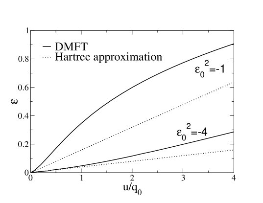
Figure 1: Dimensionless inverse correlation length of the equilibrium liquid state as function of the coupling constant (scaled by the modulation wave number $q_{0}$ for different segregation strength $\epsilon_{0}^{2}$. The DMFT results (solid lines) are compared with the leading order Hartree approximation (dashed lines). Strong deviations for small dimensionless coupling constants $u/q_{0}$ occur in the limit of weak segregation strength. Note, the results are obtained by ignoring the possibility of a fluctuation induced first order transition which will become relevant if $|\epsilon_{0}^{2}|>c(u/q_{0})^{(}2/3)$ with $c$ a constant of order unity.

In our treatment of the equilibrium behavior we have made the assumption that no phase transition to a state with long range order of $\left\langle\phi\left(\mathbf{x}\right)\right\rangle$ takes place. This is consistent with the Hartree theory which excludes a diverging correlation length for finite temperatures, and thus, excludes the possibility of a second order phase transition. However this assertion contrasts with the result found by BrazovskiiBrazovskii who showed that the model, Eq.17, undergoes a fluctuation induced first order transition to a modulated state with order parameter

$$\left\langle\phi\left(\mathbf{x}\right)\right\rangle=\phi_{0}\cos\left(\mathbf{q}_{0}\cdot\mathbf{x}\right),$$ (23)

where $\left|\mathbf{q}_{0}\right|=q_{0}$ and arbitrary but fixed direction. For small coupling constant this transition occurs if $\left|\varepsilon_{0}^{2}\right|>\frac{3}{\left(8\pi\right)^{2/3}}\left(\frac{u}{q_{0}}\right)^{2/3}$. The criterion for the glass transition discussed in this paper is very similar to the parameter values leading to the fluctuation induced first order transition. We have not analyzed both transitions within an identical theoretical approach but find in Appendix A that perturbation theory yields for the occurrence of the glass transition $\left|\varepsilon_{0}^{2}\right|\propto\left(\frac{u}{q_{0}}\right)^{3/5}$. In what follows we will always assume that the glass transition occurs instead of the fluctuation induced first order transition. In the laboratory this will likely be  a kinetic issue, that needs a nucleation theory for quantitative predictions. The results of Ref.Hohenberg, where a nucleation theory of the Brazovskii transition was developed demonstrate that indeed the nucleation kinetics of the order parameter, Eq.23 is very complex, i.e. under-cooling should be possible.

II.3.2 DMFT in the glassy state

To use the replica theory of the glassy state we have to specify the replica structure of the correlation function. We first choose a given structure and discuss its stability later. In replica space we start from the following structure of the propagators and self energies:

$$G_{\alpha\beta}\left(q\right) = K\left(q\right)\delta_{\alpha\beta}+F\left(q\right)$$

$$\Sigma_{\alpha\beta} = \Sigma_{K}\delta_{\alpha\beta}+\Sigma_{F}.$$ (24)

Inverting the matrix Dyson equation in replica space leads to:

$$K\left(q\right) = \frac{1}{\left(q-q_{0}\right)^{2}+\kappa^{2}q_{0}^{2}}$$ (25)

$$mF\left(q\right) = \frac{1}{\left(q-q_{0}\right)^{2}+\varepsilon^{2}q_{0}^{2}}-\frac{1}{\left(q-q_{0}\right)^{2}+\kappa^{2}q_{0}^{2}}$$

with the convenient definitions:

$$\kappa^{2}q_{0}^{2} = \varepsilon_{0}^{2}q_{0}^{2}-\Sigma_{K}\left(q\right)$$ (26)

$$\varepsilon^{2}q_{0}^{2} = \varepsilon_{0}^{2}q_{0}^{2}-\Sigma_{K}\left(q\right)-m\Sigma_{F}\left(q\right).$$

The diagonal elements $K\left(q\right)+F\left(q\right)$ can be interpreted as the equilibrium, liquid state correlation function and is only determined by $\varepsilon$ which can be related to the liquid state correlation length $\xi\simeq\frac{1}{\varepsilon q_{0}}$. On the other hand $F\left(q\right)=\lim_{t\rightarrow\infty}\lim_{t^{\prime}\rightarrow\infty}\left\langle\phi_{q}\left(t\right)\phi_{-q}\left(t+t^{\prime}\right)\right\rangle$ characterizes long time correlations in analogy to the Edwards-Anderson parameter.  Clearly, if $\Sigma_{F}\neq 0$ then $\kappa>\varepsilon$   and $F\left(q\right)>0$.  Depending of whether one considers $q$ values close to or away from $q_{0}$, $F\left(q\right)$ is governed by the correlation length $\xi$ or the Lindemann length of the glass $\lambda_{0}=q_{0}^{-1}\left(\kappa^{2}-\varepsilon^{2}\right)^{-1}$, respectively. The physical significance of  $\lambda_{0}$ is the length scale over which defects and imperfections of  an crystalline state can wander after long time was discussed in Ref.SWW00 . Finally, the correlation function $K\left(q\right)$ (which is solely determined by the short length $\frac{1}{\kappa q_{0}}<\xi$) is the response function of a local perturbation. Obviously, any response of the glassy system is confined to very small length scales even though the instantaneous correlation length can be considerable. This is a clear reflection of the violation of the fluctuation dissipation relation within the replica approach. Averaging these functions over momenta gives:

$$\overline{K} = \int\frac{d^{3}q}{\left(2\pi\right)^{3}}K\left(q\right)=\frac{q_{0}}{2\pi\kappa},$$

$$\overline{F} = \int\frac{d^{3}q}{\left(2\pi\right)^{3}}F\left(q\right)=\frac{q_{0}}{2\pi m}\left(\frac{1}{\varepsilon}-\frac{1}{\kappa}\right).$$ (27)

The  auxiliary local Hamiltonian is

$$\mathcal{H}=\frac{1}{2}\sum_{ab}\mathcal{J}_{ab}\phi_{a}\phi_{b}+\frac{uq_{0}^{-3}}{4}\sum_{a}\phi_{a}^{4}.$$ (28)

Within DMFT we then find for its correlation function

$$\mathcal{G}=\overline{K}\delta_{ab}+\overline{F}.$$ (29)

In addition, the Weiss field is given by:

$$\mathcal{J}_{\alpha\beta}=\mathcal{J}\delta_{\alpha\beta}-\mathcal{C}.$$ (30)

These relations together with Eq.27 can be used to express the Weiss fields in terms of the $\varepsilon$ and $\kappa$:

$$\mathcal{J} = \frac{2\pi\kappa+\varepsilon_{0}^{2}-\kappa^{2}}{q_{0}}$$

$$\mathcal{C} = \frac{2\pi\left(\kappa-\varepsilon\right)+\varepsilon^{2}-\kappa^{2}}{mq_{0}}.$$ (31)

Thus, we have to determine $\overline{K}$ and $\overline{F}$ for given $\mathcal{J}$ and $\mathcal{C}$ and make sure that the latter are chosen such that Eqs.27 and 31 are fulfilled.

The partition sum of the local problem is given by

$$\mathcal{Z}\left(m\right)=\int d^{m}\phi e^{-\sum_{\alpha=1}^{m}\mathcal{H}_{0}\left[\phi_{\alpha}\right]+\frac{1}{2}\mathcal{C}\left(\sum_{\alpha}\phi_{\alpha}\right)^{2}},$$ (32)

where $\mathcal{H}_{\mathrm{0}}\left[\phi_{\alpha}\right]=\frac{1}{2}\mathcal{J}\phi_{a}^{2}+\frac{uq_{0}^{-3}}{4}\phi_{a}^{4}$.  $d^{m}\phi$ refers to the fact that $\phi$ is an $m$-component vector and the integral goes over an $m$-dimensional space with arbitrary $m$. The coupling between different replicas can be eliminated by performing a Hubbard-Stratonovich transformation, which leads to

$$\mathcal{Z}\left(m\right)=\int\frac{d\lambda}{\sqrt{2\pi\mathcal{C}}}e^{-\frac{\lambda^{2}}{2\mathcal{C}}}\Omega\left(\lambda\right)^{m}$$ (33)

where

$$\Omega\left(\lambda\right)=\int d\phi e^{-\left(\mathcal{H}_{0}\left[\phi\right]+\lambda\phi\right)}$$ (34)

is the equilibrium partition function however in an external field $\lambda$, with Gaussian distribution function.

In order to determine the propagators of the local problem, we consider the sum of the diagonal elements

$$\sum_{a}\overline{G}_{aa}=m\left(\overline{K}+\overline{F}\right)\$$ (35)

which is equal to $-2\frac{\partial\log\mathcal{Z}\left(m\right)}{\partial\mathcal{J}}$, yielding

$$\overline{K}+\overline{F}=-2\int\frac{d\lambda e^{-\frac{\lambda^{2}}{2\mathcal{C}}}\Omega\left(\lambda\right)^{m-1}}{\mathcal{Z}\left(m\right)\sqrt{2\pi\mathcal{C}}}\frac{\partial}{\partial\mathcal{J}}\Omega\left(\lambda\right).$$ (36)

The derivative with respect to $\mathcal{J}$ leads to

$$\frac{\partial}{\partial\mathcal{J}}\Omega\left(\lambda\right)=-\frac{1}{2}\int d\phi e^{-\left(\frac{1}{2}\mathcal{J}\phi^{2}+\frac{uq_{0}^{-3}}{4}\phi^{4}+\lambda\phi\right)}\phi^{2}$$ (37)

which gives the final expression for the diagonal element of the replica correlation function

$$\overline{K}+\overline{F}=\frac{\int\frac{d\lambda}{\sqrt{2\pi\mathcal{C}}}e^{-\frac{\lambda^{2}}{2\mathcal{C}}}\Omega\left(\lambda\right)^{m}\left\langle\phi^{2}\right\rangle_{\lambda}}{\mathcal{Z}\left(m\right)}$$ (38)

with

$$\left\langle\phi^{2}\right\rangle_{\lambda}=\frac{\int d\phi e^{-\left(\frac{1}{2}\mathcal{J}\phi^{2}+\frac{uq_{0}^{-3}}{4}\phi^{4}+\lambda\phi\right)}\phi^{2}}{\Omega\left(\lambda\right)}.$$ (39)

In addition we also need to determine the off diagonal elements in replica space of the correlation function. We use

$$\sum_{a,b}\overline{G}_{ab}=m\overline{K}+m^{2}\overline{F}\$$ (40)

which equals to $2\frac{\partial\log\mathcal{Z}\left(m\right)}{\partial\mathcal{C}}$ and obtain an equation which can be used to determine the off diagonal elements $\overline{F}$

$$\overline{K}+m\overline{F}=-\frac{\int\frac{d\lambda}{\sqrt{2\pi\mathcal{C}}}e^{-\frac{\lambda^{2}}{2\mathcal{C}}}\Omega\left(\lambda\right)^{m}\mathcal{C}^{-1}\left\langle\phi\right\rangle_{\lambda}\lambda.}{\mathcal{Z}\left(m\right)}$$ (41)

Evidently, Eqs.38 and 41 are only independent if $m$ differs from $1$.

We next analyze these equations for small but finite $m-1$. This can be done by expanding Eqs.38 and 41 into a Taylor series for small $m-1$ and comparing order by order. First we consider the zeroth order term and find that both equations yield for $m=1$, the results for the liquid state which determine $\varepsilon$. The next step is to consider the first corrections linear in $m-1$. This allows us to check whether there are nontrivial solutions for $\kappa>\varepsilon$ and thus for the off diagonal self energy and long time correlation function.

The difference between Eqs.38 and 41 gives

$$\overline{F}=\frac{\int\frac{d\lambda}{\sqrt{2\pi\mathcal{C}}}e^{-\frac{\lambda^{2}}{2\mathcal{C}}}\Omega\left(\lambda\right)^{m}\left(\left\langle\phi^{2}\right\rangle_{\lambda}+\mathcal{C}^{-1}\left\langle\phi\right\rangle_{\lambda}\lambda\right)}{\left(1-m\right)\mathcal{Z}\left(m\right)}.$$ (42)

Expanding the numerator for $m$ close to $1$ gives

$$\overline{F}=\frac{\delta I\ }{\mathcal{Z}\left(m=1\right)}$$ (43)

with

$$\delta I=-\int\frac{d\lambda\left(\mathcal{C}^{-1}\left\langle\phi\right\rangle_{\lambda}\lambda+\left\langle\phi^{2}\right\rangle_{\lambda}\right)e^{-\frac{\lambda^{2}}{2\mathcal{C}}}\Omega\left(\lambda\right)\log\Omega\left(\lambda\right)}{\sqrt{2\pi\mathcal{C}}}.$$ (44)

As expected, it follows that $\overline{F}=0$ if $\kappa=\varepsilon$, where $\mathcal{C}=0$. This can be seen from the expansion $\left\langle\phi\right\rangle_{\lambda}\simeq-\left\langle\phi^{2}\right\rangle_{\lambda}\lambda$, valid for small $\lambda$ and by substituting $\mu=\lambda/\sqrt{\mathcal{C}}$. It follows that

$$\overline{F}\left(\kappa=\varepsilon\right)\ \propto\int\frac{d\mu}{\sqrt{2\pi}}e^{-\frac{\mu^{2}}{2}}\left(1-\mu^{2}\right)=0.$$ (45)

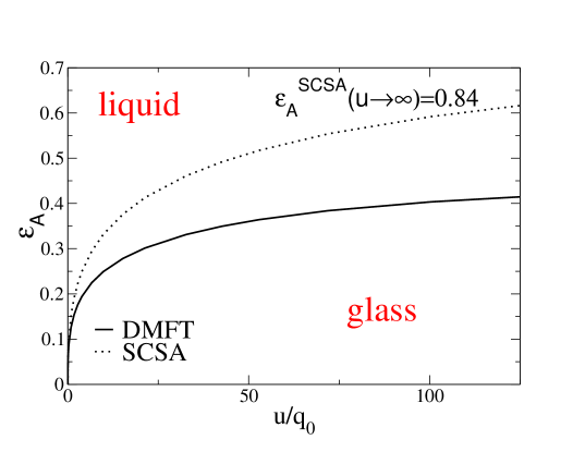
Figure 2: Dimensionless inverse correlation length as function of the coupling constant at the dynamical glass transition $\epsilon_{A}$ obtained within the DMFT, in comparison with the result of the self consistent screening approximation. For large $u$ a universal value of the correlation length (in units of $q_{0}^{-1}$ for glassiness results, whereas the critical value of the spatial correlations to reach a glassy state increases considerably in the weak coupling limit.

In Fig.2 we show our results for the dimensionless inverse correlation length $\varepsilon_{\mathrm{A}}=\varepsilon\left(u_{\mathrm{A}}\right)$ at the onset of glassiness. We have to distinguish the two different regimes of strong and weak phase separation, characterized by $\left|\varepsilon_{0}^{2}\right|>1$ and $\left|\varepsilon_{0}^{2}\right|<1$, respectively.  In the case of strong phase separation we find a universal  value $\varepsilon_{\mathrm{A}}\simeq 0.45$. The universality of this result is in qualitative agreement with results obtained with perturbation theory which also gives such a generic value which is however numerically larger ($\varepsilon_{\mathrm{A}}\simeq 0.8385$). In addition we obtain that at the transition the ratio $\kappa_{\mathrm{A}}/\varepsilon_{\mathrm{A}}$ $\simeq 3.5$, which is close to the result $\kappa_{\mathrm{A}}/\varepsilon_{\mathrm{A}}=3.1$, obtained within perturbation theory.The onset of glassiness in the model Eq.17 occurs in the strong phase separation limit and, for given $q_{0}$, is uniquely determined by the value of the correlation length $\xi=\left(\varepsilon q_{0}\right)^{-1}$, and not explicitly dependent on $u$ or $T$.  The exact solution of the dynamic mean field problem leads to the interesting result that this value for $\xi$ is larger than what follows within perturbation theory. For small $\frac{u}{q_{0}}$, the result of the perturbation theory is $\varepsilon_{\mathrm{A}}\simeq 0.42\left(\frac{u}{q_{0}}\right)^{2/5}$. In this limit the DMFT gives the interesting result that $\varepsilon_{\mathrm{A}}$ is larger than the value obtained within perturbation theory. The effect is small and numerically hard to identify. It implies that the criterion for glassiness as obtained within DMFT becomes very close to the one found by Brazovskii for the fluctuation induced first order transition. Most important  however is that we do indeed find that there is a nontrivial solution $\kappa>\varepsilon$. The emergence of a self generated glassy state is therfore not a consequence of the perturbative solution used in Refs.SW00, ; SWW00, . Our calculation is performed for a temperature $T=1$. We can reintroduce the temperature into the calculation by substituting $u\rightarrow uT$. A critical value for $u$ leads to a temperature $T_{\mathrm{A}}$ (for fixed $u$) where within mean field theory an exponential number of metastable states emerges.

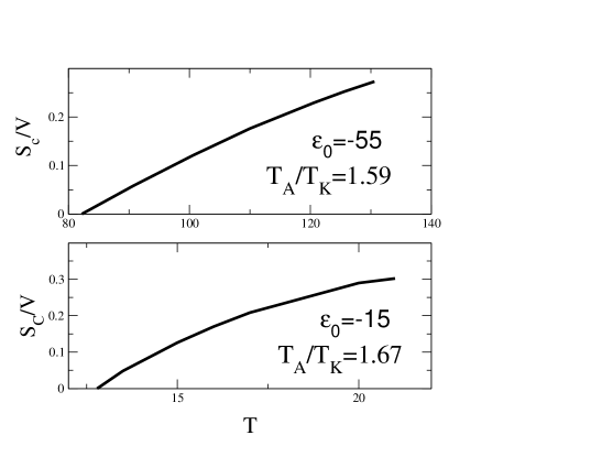
Figure 3: Configurational entropy density $S_{c}/V$ (with system volume $V$) as function of temperature for two different values of the segregation strength $\epsilon_{0}^{2}$.

Once the correlation functions are determined we can use the fact that the functional $\Phi\left[G\right]$ is the same for the local problem as well as the original one to obtain

$$F\left(m\right)=\mathcal{F}\left(m\right)+\frac{T}{2m}\left(\mathrm{tr\log}G^{-1}-a_{0}^{-d}\mathrm{Tr\log}\overline{G}^{-1}\right).$$ (46)

Here $\mathrm{Tr}$ refers to the trace over replicas, but  does not include the momentum integration, as opposed to $\mathrm{tr}$ which corresponds to a trace with respect to all degrees of freedom. Finally, $\mathcal{F}\left(m\right)=-\frac{T}{m}\log\mathcal{Z}\left(m\right)$ is the counter part of $F\left(m\right)$ for the local problem. Using Eq.6 an expression for the configurational entropy follows:

$$\frac{S_{c}}{V} = -\frac{1}{2}\sum_{q}[\log\mathbf{(}1-\frac{F(q)}{G(q)}\mathbf{)+}\frac{F(q)}{G(q)}]-\frac{a_{0}^{-d}}{2}\log\left(\frac{\kappa}{\varepsilon}\right)$$ (47)

$$+\frac{a_{0}^{-d}}{2}(1-\frac{\varepsilon}{\kappa})-a_{0}^{-d}\left.\frac{\partial\log\mathcal{Z}\left(m\right)/m}{\partial m}\right|_{m\rightarrow 1},$$

where $G(q)=K(q)+F(q)$ and

$$\left.\frac{\partial\mathcal{Z}\left(m\right)}{\partial m}\right|_{m\rightarrow 1}=\int\frac{d\lambda}{\sqrt{2\pi\mathcal{C}}}e^{-\frac{\lambda^{2}}{2\mathcal{C}}}\Omega\left(\lambda\right)\log\Omega\left(\lambda\right).$$ (48)

As expected, in the limit $\kappa\rightarrow\varepsilon$ without glassy long time correlations, it follows $\mathcal{Z}\left(1\right)=\Omega\left(0\right)$ as well as $\left.\frac{\partial\mathcal{Z}\left(m\right)}{\partial m}\right|_{m\rightarrow 1}=\Omega\left(0\right)\log\Omega\left(0\right)$ and $F(q)$ goes to zero, leading to $S_{c}\left(\kappa=\varepsilon\right)=0$.  The configurational entropy is finite only for nontrivial solutions $\kappa>\varepsilon$. The temperature, $T_{\mathrm{A}}$, where this happens for the first time is equal to the dynamic transition temperature of the system. The result for $S_{c}\left(T\right)$ also enables us to determine the Kauzmann temperature, $T_{\mathrm{K}}<T_{\mathrm{A}}$, where $S_{\rm c}$ vanishes. In Fig.3, we show $S_{\rm c}(T)$ for two different $\left|\varepsilon_{0}^{2}\right|.$ The configurational entropy vanishes as $T_{\mathrm{K}}$ is approached: $S_{c}\propto T-T_{\mathrm{K}}$. The regime $(T_{\rm A}-T_{\rm K})/T_{\rm A}$ between the onset of slow dynamics and entropy crisis increases for decreasing strength of the phase separation.

II.4 Stability of the solution

An important simplification of our approach resulted from the simple form, Eq.24, of the correlation function in replica space. All diagonal elements as well as all off diagonal elements are assumed to be identical. Whether this assumption is indeed stable can be addressed by evaluating the eigenvalues of the stability matrix

$$\widehat{H}_{\alpha\beta;\gamma\delta}=\frac{\delta^{2}F}{\delta G^{\alpha b}\left(q\right)\delta G^{\gamma\delta}\left(q^{\prime}\right)}.$$ (49)

If there are negative eigenvalues of $\widehat{H}$ our assumption for the replica structure is unstable. Following Ref.dAT78, we find that the lowest eigenvalue with respect to the replica indices is determined by the lowest eigenvalue of the matrixWSW02

$$\widehat{h}_{\mathbf{q,q}^{\prime}}=\delta\left(\mathbf{q-q}^{\prime}\right)K^{-2}\left(q\right)+v_{0}$$ (50)

in momentum space, where $v_{0}=\frac{\delta^{2}\Phi}{\delta\overline{G}^{\alpha\beta}\delta\overline{G}^{\alpha\beta}}-2\frac{\delta^{2}\Phi}{\delta\overline{G}^{\alpha\beta}\delta\overline{G}^{\alpha\delta}}+\frac{\delta^{2}\Phi}{\delta\overline{G}^{\alpha\beta}\delta\overline{G}^{\gamma\delta}}$ with distinct $\alpha,\beta,\gamma$ and $\delta$. In deriving this result we started from Eq.8 but used the fact that the functional $\Phi$ only depends on the momentum averaged correlation function, such that $v_{0}$ becomes momentum independent. Eq.50 is similar to the Schrödinger equation in momentum space of a single particle with bare Hamiltonian $K^{-2}\left(q\right)$ and local potential $v_{0}$. The lowest eigenvalue, $E$, of this problem is given by

$$1=v_{0}\int\frac{d^{3}q}{\left(2\pi\right)^{3}}\left(K^{-2}\left(q\right)+E\right)^{-1}.$$ (51)

This equation can be analyzed if we find a way to calculate $v_{0}$ which, due to Eq.9, is determined by the first derivative of the self energy with respect to the correlation function $\frac{\delta\Sigma_{\alpha\beta}}{\delta\overline{G}_{\gamma\delta}}$. This derivative can be evaluated by following closely Baym and KadanoffKB70 . First we add to the local Hamiltonian an additional term $-\sum_{\alpha\beta}U_{\alpha\beta}\phi_{a}\phi_{\beta}$ and analyze all correlation functions for finite $U$. At the end we  will take the limit $U\rightarrow 0$ and the correlation function has the simple structure Eq.50. For finite $U$, the correlation function is determined from the function $\mathcal{Z}\left[U\right]$:

$$\overline{G}_{\alpha\beta}\left[U\right]=\left\langle\phi_{\alpha}\phi_{\beta}\right\rangle=-\frac{\delta\log\mathcal{Z}\left[U\right]}{\delta U_{\alpha\beta}}$$ (52)

The self energy is a functional of only $\overline{G}\left[U\right]$ and not of $U$ explicitly such that

$$\frac{\delta\Sigma_{\alpha\beta}}{\delta U_{\gamma\delta}}=\sum_{\mu\nu}\frac{\delta\Sigma_{\alpha\beta}}{\delta\overline{G}_{\mu\nu}}\frac{\delta\overline{G}_{\mu\nu}}{\delta U_{\gamma\delta}}$$ (53)

If we furthermore introduce

$$L_{\alpha\beta;\gamma\delta} = \frac{\delta G_{\alpha\gamma}}{\delta U_{\delta\beta}}$$ (54)

$$= \left\langle\phi_{\alpha}\phi_{\beta}\phi_{\gamma}\phi_{\delta}\right\rangle-\left\langle\phi_{\alpha}\phi_{\gamma}\right\rangle\left\langle\phi_{\delta}\phi_{\beta}\right\rangle$$

which can be evaluated explicitly once $U=0$, one finds

$$\sum_{\mu\nu}\left(G_{\alpha\mu}^{-1}G_{\nu\gamma}^{-1}-\frac{\delta\Sigma_{\mu\nu}}{\delta\overline{G}_{\alpha\gamma}}\right)L_{\alpha\beta;\gamma\delta}=\delta_{\mu\delta}\delta_{\beta\nu}$$ (55)

which determines $\frac{\delta\Sigma_{\mu\nu}}{\delta\overline{G}_{\alpha\gamma}}$ and thus $v_{0}$.

Applying this approach to the Brazovskii model we find that the replica structure is marginally stable at the temperature $T_{\mathrm{A}}$ where the glassy state occurs for the first time. Below $T_{\mathrm{A}}$ the replica symmetric ansatz Eq.50 becomes unstable however it can be made stable if the replica index $m$ does not approach $1$ anymore but rather takes a value $m=\frac{T}{T_{\mathrm{eff}}}$ which defines the effective temperature $T_{\mathrm{eff}}$ of the glass. This is a situation similar to one step replica symmetry breaking with break point given by $m$.Mon95 A detailed discussion of this issue is presented in Ref.WSW02, .

Stability of the replica symmetric  ansatz was only possible because we consistently made the assumption of the dynamical mean field theory. Going beyond the local approach, for example by using cluster DMFT techniques, enables one to study whether or not nonlocal phenomena change the replica structure of the theory.

III Conclusions

Based on the recent development in the theory of strongly interacting electron systems we developed a dynamic mean field theory for self generated glasses in a continuum field theory model. The key assumption of our approach, which applies to physical systems with short range higher order virial coefficients, is that glass formation is the consequence of predominantly local correlations. It is then possible to map the problem onto a purely local theory with same interaction and with a Gaussian part of the energy which is determined self consistently.  The comparatively simple approach can easily be applied to multi component systems.  Most importantly, recent developments in the cluster DMFT approach allow one to generalize this theory to include at least short range non-local effects. Owing to its local character a generalization of the present treatment to include spatially inhomogeneous states (corresponding with instantons) and thereby explicitly treat the mosaic formation predicted in random first order transitions seems well within reach.

IV Acknowledgments

We would like to thank Giulio Biroli, Paul Goldbart and Harry Westfahl Jr. for helpful discussions. This research was supported by an award from Research Corporation (J.S.), the Institute for Complex Adaptive Matter, the Ames Laboratory, operated for the U.S. Department of Energy by Iowa State University under Contract No. W-7405-Eng-82 (S.W. and J. S.), and the National Science Foundation grants DMR-0096462 (G. K.) and CHE-9530680 (P. G. W.).

Appendix A Self-consistent screening approximation

In this appendix we summarize the solution of the Brazovskii model within self-consistent screening approximation of Refs.SW00, ; SWW00, . In Ref. SW00, a complete numerical solution of the self consistent screening approximation was developed which did not make any assumption with respect to the momentum dependence of the self energy.  It was found that $\Sigma\left(q\right)$ does weakly depend on $q$ for $q<2q_{0}$ allowing to approximate $\Sigma\left(q\right)\simeq\Sigma\left(q_{0}\right)$ momentum independent. This simplification was helpful to develop an analytical solution of the same problem, presented in Ref.SWW00, . Here we will show that the results of Ref.SWW00, can easily be re-derived by performing a dynamic mean field theory where the local problem is solved within perturbation theory.

It is useful to first summarize the problems which result in a perturbative treatment of the problem,  something that can already be seen in the liquid state. Consider a given Feynman diagram for the self energy of a theory with interaction $u\phi^{r}$ ($r=4$ in our case). The number of internal lines is $I_{n}=\frac{1}{2}\left(nr-2\right)$, whereas the number of internal momentum integrations of the original theory is $L_{n}=I_{n}-\left(n-1\right)=n\left(\frac{r}{2}-1\right)$. In a local theory we have for each running line a contribution $q_{0}^{-3}\overline{G}$ (i.e. we replace $G\left(q\right)$ by its momentum averaged value). Thus, we obtain for a contribution to the self energy of order $n$

$$\delta\Sigma^{\left(n\right)}\sim u^{n}\left(q_{0}^{3}\right)^{L_{n}}\left[q_{0}^{-3}\overline{G}\right]^{I_{n}}$$ (56)

Using $r=4$ and $\overline{G}$ of Eq.20 it follows $\delta\Sigma^{\left(n\right)}\sim\frac{uq_{0}}{\varepsilon}\left(\frac{u}{q_{0}\varepsilon^{2}}\right)^{n-1}$. Clearly, in the limit of $\varepsilon<1$, where glassiness was found in Refs.SW00, ; SWW00, , the perturbation series is a sum terms which are increasingly larger in magnitude.e. strongly divergent. The self consistent screening approximation corresponds to the sum

$$\Sigma_{\mathrm{SSC}}\sim-\sum_{n=1}^{\infty}\left(-1\right)^{n}\delta\Sigma^{\left(n\right)}\propto-\frac{uq_{0}}{\varepsilon}\frac{1}{1+\frac{u}{q_{0}\varepsilon^{2}}}.$$ (57)

Even though $\Sigma_{\mathrm{SSC}}=-\ q_{0}^{2}\varepsilon$ is small for small $q_{0}\varepsilon^{2}$, it is not clear at all whether this procedure leads to reliable results, making evident the need to use a method not based on the summation of diagrams.

Using the replica approach for the local problem we obtain within the self consistent screening approximation for the local self energies:

$$a_{0}^{3}\Sigma_{K} = -2\left(D_{K}K+D_{K}F+D_{F}K\right)$$

$$a_{0}^{3}\Sigma_{F} = -2D_{F}F$$ (58)

with collective propagators

$$D_{K} = \frac{1}{q_{0}^{3}u^{-1}+\Pi_{K}},$$

$$D_{F} = -\frac{\Pi_{F}D_{K}^{2}}{\ 1+\Pi_{F}D_{K}}\ ,$$ (59)

where $\Pi_{K}=K^{2}+2KF$ and $\Pi_{F}=F^{2}$. This corresponds to the summation of bubble diagrams as summarized in detail in Ref.SWW00, and follows from the functional

$$\Phi[G]=a_{0}^{-d}{\rm Tr}{\rm log}D^{-1}$$ (60)

with $D_{ab}=D_{K}\delta_{ab}+D_{F}$. Since we are solving a classical (time independent) local problem we do not need to perform any momentum integrations in the evaluation of the diagrams.

Using the expressions for the momentum averaged propagator, Eq.27, we find for $\Sigma_{F}=\left(\kappa^{2}-\varepsilon^{2}\right)q_{0}^{2}$:  

$$a_{0}^{3}\Sigma_{F}=\frac{4\pi\varepsilon}{q_{0}\left(\ 1+\varepsilon^{2}v^{-1}\right)}\frac{\ \left(1-\frac{\varepsilon}{\kappa}\right)^{3}}{\varepsilon^{2}v^{-1}+1-\left(1-\frac{\varepsilon}{\kappa}\right)^{2}},\$$ (61)

where $v=\frac{1}{\left(2\pi\right)^{2}}uq_{0}^{2}a_{0}^{3}$. With the choice $a_{0}=\ \frac{\pi^{2/3}}{2^{1/3}}q_{0}^{-1}\simeq 1.7q_{0}^{-1}$ this agrees with the result of Ref.SWW00, , analyzed in the strong coupling limit $v^{-1}\rightarrow 0$. In what follows we simply use $a_{0}=q_{0}^{-1}$ to be able to compare the results of the self consistent screening with the solution of the DMFT approach of this paper. In the limit $v^{-1}\rightarrow 0$ a solution $\kappa>\varepsilon$ exists for the first time if $\varepsilon<\varepsilon_{\mathrm{A}}\simeq 0.84$. At the transition $\kappa_{\mathrm{A}}\simeq 3.1\varepsilon_{\mathrm{A}}$.  A detailed physical discussion of these results is given in Ref.SWW00, . For weak coupling it follows $\varepsilon_{\mathrm{A}}\simeq 0.422\left(\frac{u}{q_{0}}\right)^{2/5}$ with $\kappa_{\mathrm{A}}\simeq 2.19\varepsilon_{\mathrm{A}}$.

References

- (1) D. N. Argyriou, J. W. Lynn, R. Osborn, B. Campbell, J. F. Mitchell, U. Ruett, H. N. Bordallo, A. Wildes, C. D. Ling, Physical Review Letters 89, 036401 (2002).
- (2) A. J. Millis, Phys. Rev. B 53, 8434 (1996).
- (3) E. Dagotto, T. Hotta, and A. Moreo, Physics Reports (2001).
- (4) M.-H. Julien, F. Borsa, P. Carretta, M. Horvatic, C. Berthier, and C. T. Lin, Phys. Rev. Lett. 83, 604 (1999).
- (5) A. W. Hunt, P. M. Singer, K. R. Thurber, and T. Imai, Phys. Rev. Lett. 82, 4300 (1999).
- (6) N. J. Curro, P. C. Hammel, B. J. Suh, M. Hücker, B. Büchner, U. Ammerahl, and A. Revcolervschi, Phys. Rev. Lett. 85, 642 (2000).
- (7) J. Haase, R. Stern, C. T. Milling, C. P. Slichter, and D. G. Hinks, Physica C 341, 1727 (2000).
- (8) N. J. Curro, Journal of Physics and Chemistry of Solids 63, 2181(2002).
- (9) Ch. Niedermeyer, C. Bernhard, T. Blasius, A. Golnik, A. Moodenbaugh, and J. I. Budnik, Phys. Rev. Lett. 80, 3843 (1998).
- (10) C. Panagopoulos, J. L. Tallon, B. D. Rainford, T.Xiang, J. R. Cooper, and C. A. Scott, Phys. Rev. B 66, 064501 (2002).
- (11) J. L. Tallon, J. W. Loram, C. Panagopoulos, cond-mat/0211048, to appear in J. Low Temp. Phys.
- (12) R. Monasson, Phys. Rev. Lett. 75, 2875 (1995).
- (13) M. Mézard and G. Parisi, Phys. Rev. Lett. 82, 747 (1999). (1989).
- (14) Y. Singh, J. P. Stoessel, and P. G. Wolynes, Phys. Rev. Lett. 54, 1059 (1985).
- (15) T. R. Kirkpatrick and P. G. Wolynes, Phys. Rev. A 35, 3072 (1987).
- (16) T. R. Kirkpatrick and P. G. Wolynes, Phys. Rev. B 36, 8552 (1987).
- (17) T. R. Kirkpatrick and D.Thirumalai, and P. G. Wolynes, Phys. Rev. A 40, 1045 (1989).
- (18) T. R. Kirkpatrick and D. Thirumalai, Phys. Rev. Lett. 58, 2091 (1987).
- (19) R. B. Laughlin and D. Pines, Proc. of the Natl. Acad. of Sciences 97 27 (2000).
- (20) T. V. Ramakrishnan and M. Yussouff, Phys. Rev. B 194, 2775 (1979); M. Youssouff, Phys. Rev. B 23, 5871 (1983).
- (21) Q. Si and J. L. Smith, Phys. Rev. Lett. 77, 3391 (1996).
- (22) R. Chitra and G. Kotliar, Phys. Rev. B 63, 115110 (2001).
- (23) M. H. Hettler, A. N. Tahvildar-Zadeh, M. Jarrell, T. Pruschke, H. R. Krishnamurthy, Phys. Rev. B 58, R7475 (1998).
- (24) A. I. Lichtenstein and M. I. Katsnelson, Phys. Rev. B 63, R9283 (2000).
- (25) G. Biroli and G. Kotliar, Phys. Rev. B 65, 155112 (2002).
- (26) A. V. Lopatin and L. B. Ioffe, Phys. Rev. B 66, 174202 (2002)
- (27) G. Baym and L. P. Kadanoff, Phys. Rev 124, 287 (1961); G. Baym, Phys. Rev 127, 1391 (1962).
- (28) J. Schmalian and P. G. Wolynes, Phys. Rev. Lett. 85, 836 (2000).
- (29) J.-P. Bouchaud, L. Cugliandolo, J. Kurchan, M. Mézard, Physica A, 226, 243 (1996).
- (30) P. L. Geissler and D. R.Reichman, cond-mat/0304254
- (31) H. Westfahl Jr., J. Schmalian, and P. G. Wolynes, Phys. Rev. B 64, 174203 (2001).
- (32) H. Westfahl Jr., J. Schmalian, and P. G. Wolynes, preprint
- (33) L. F. Cugliandolo, J. Kurchan, Phys. Rev. Lett. 71, 173 (1993).
- (34) W. Götze, in Liquids, Freezing and Glass Transition, ed. J.-P. Hansen, D. Levesque and J. Zinn-Justin (North-Holland, Amsterdam, 1991), p. 287.
- (35) J. P. Hansen and I. R. McDonald, Theory of simple liquids, Academic Press, London, N.Y., San Francisco, 1976.
- (36) D. Vollhardt, in Correlated Electron Systems, edited by V.J. Emery (World Scientific, Singapore, 1993).
- (37) A. Georges, G. Kotliar, W. Krauth, and M. J. Rozenberg, Rev. Mod. Phys. 68, 13-125 (1996).
- (38) R. T. Deam and S. F. Edwards, Phil. Trans. R. Soc. 280A, 317 (1976).
- (39) P. M. Goldbart, H. E. Castillo, and A. Zippelius, Adv. Phys. 45, 393 (1996).
- (40) T. Kirkpatrick and D. Thirumalai, J. Phys. A Math.-Gen. 22, L49 (1989).
- (41) D. Kivelson, S. A. Kivelson, X. L. Zhao, Z. Nussinov, and G. Tarjus, Physica A 219, 27 (1995).
- (42) F. H. Stillinger, J. Chem. Phys. 78, 4654 (1983).
- (43) M. W. Deem and D. Chandler, Phys. Rev. E 49, 4268 (1994).
- (44) S. A. Brazovskii, Zh. Exp. Teor. Fiz. 68, 175 (1975) [Sov. Phys. JEPT 41, 85 (2975)].
- (45) L. Leibler, Macromolecules 13, 1602 (1980).
- (46) G. H. Fredrickson and E. Helfand, J. Chem. Phys. 87, 697 (1987).
- (47) V. J. Emery and S. A. Kivelson, Physica 209C, 597 (1993).
- (48) S. Wu, H. Westfahl Jr., J. Schmalian, P. G. Wolynes, Chem. Phys. Lett. 359, 1 (2002).
- (49) P. C. Hohenberg and J. B. Swift, Phys. Rev. E 52, 1828 (1995).
- (50) J. R. L. de Alameida and D. J. Thouless, J. Phys. A 11, 983 (1978).
- (51) as defined in this paper differs from the one of Ref.[31] by a factor .