Magnetism, Critical Fluctuations and Susceptibility Renormalization in Pd

Abstract

Some of the most popular ways to treat quantum critical materials, that is, materials close to a magnetic instability, are based on the Landau functional. The central quantity of such approaches is the average magnitude of spin fluctuations, which is very difficult to measure experimentally or compute directly from the first principles. We calculate the parameters of the Landau functional for Pd and use these to connect the critical fluctuations beyond the local-density approximation and the band structure.

The physics and materials science of weak itinerant ferromagnetic metals and highly renormalized paramagnets near magnetic instabilities has attracted renewed theoretical interest. This is a result of recent discoveries of materials with highly non-conventional metallic properties, especially, non-Fermi liquid scalings, metamagnetic behavior, and unconventional superconductivity, in several cases co-existing with ferromagnetism. Discoveries in the last three years alone include the co-existing ferromagnetism and superconductivity of ZrZn₂[1], UGe₂[2],URhGe₂[3], high pressure $\epsilon$-Fe[5], and the metamagnetic quantum critical point in Sr₃Ru₂O₇ [4].

Unfortunately, although model theories have been put forth, there is still not an established material specific (first principles) theoretical understanding of these phenomena. One difficulty is the usual starting point for first principles theories, density functional theory (DFT) as implemented in the local density approximation (LDA). This already includes most spin degrees of freedom, including dynamical fluctuations, as evidenced by its formally exact description of the uniform electron gas as well as its well documented success in accurately describing a wide variety of itinerant magnetic materials. However, the electron gas, upon which most density functionals are built, is not near any critical point for densities relevant to the solid state, and furthermore the proximity to itinerant magnetism of a metal is an extremely non-local quantity, in particular depending on the electronic density of states at the Fermi level $N(E_{F})$. Therefore, the exact DFT, which by definition includes all fluctuations and describes the ground state magnetization exactly, is likely to be extremely nonlocal and probably nonanalytical for the materilas near a quantum critical point.

On the other hand, the LDA, while providing a good description of most itinerant ferromagnets that are not near critical points, fails to include the soft critical fluctuations in the materials of interest here. Since fluctuations are generically antagonistic to ordering, the result is that magnetic moments and magnetic energies of weak itinerant ferromagnets near critical points are overestimated in the LDA, as opposed to LDA’s failure to describe Mott-Hubbard insulators where the LDA underestimates the tendency to magnetism. Recent examples include Sc₃In[6], Ni₃Al[13], NaCo₂O₄[8], and ZrZn₂[9]. Similarly, susceptibilities of paramagnets near critical points are underestimated. Furthermore, there is an overlap region where the LDA predicts ferromagnetism for paramagnetic materials. This interesting class includes FeAl[11, 12], Ni₃Ga[13], and Sr₃Ru₂O₇[7] (as mentioned, this latter material shows a metamagnetic quantum critical point). The basic theoretical difficulty in correcting the LDA for these materials is that there is some unknown and possibly strongly material dependent cross-over in energy (and possibly non-trivially in momentum) separating quantum critical fluctuations, not included in the LDA, from the dynamical fluctuations that are included in the LDA. Qualitatively, this may be understood from the fact that the LDA is based on the properties of the uniform electron gas, which is far from any magnetic critical point at densities relavent for solids, the consequence being a mean-field-like description of magnetism near critical points. Thus the underlying reason for the failure of the LDA to describe these systems is very different from the failures in the well-known class of Coulomb correlated materials, such as the Mott-Hubbard insulators. There, the basic problem is the neglect of some electron-electron interactions, and can often be largely corrected at the static level, e.g. via approaches like LDA+U. It is worth noting that these dynamical fluctuations are responsible not only for the suppression of the magnetic ordering, but also for unusual transport properties of quantum critical materials, deviating from the conventional Fermi liquid behavior, for mass renormalization, and even for superconductivity in some systems. Many of these issues have been addressed recently in theoretical papers, utilizing idealized models of various kinds. However, a quantitative link between such models and actual material characteristics is still missing.

We attempt to build a bridge between such theories and the LDA. We concentrate on the question of what kind of material-specific understanding, relevant for quantum criticality, can be extracted from the LDA calculations. Primarily, we focus here on Pd. This is perhaps the best studied high susceptibility paramagnet[14, 15, 16, 17], and in fact a number of theories related to spin fluctuations have been elucidated using this material. Furthermore, itinerant ferromagnetism appears in Pd at 2.5% Ni doping[18]. We present highly accurate calculations of the static magnetic susceptibility for Pd and find that, indeed, the LDA overestimates the tendency to magnetism. We also estimate the r.m.s. magnitude of spin fluctuations (paramagnons) in Pd, needed to reduce the calculated susceptibility to reproduce experiment, and show that it is compatible with that which might be estimated from LDA susceptibility $via$ the fluctuation-dissipation theorem with a reasonable ansatz for the cut-off momentum.

We have performed electronic structure calculations using the self consistent full potential linearized augmented plane wave (FLAPW)[19] method within the density functional theory (DFT)[20]. The local density approximation (LDA) of Perdew and Wang[21] and the Generalized Gradient Approximation (GGA) of Perdew, Burke, and Ernzerhof[22] were used for the correlation and exchange potentials. Calculations were performed using the WIEN2k package[23]. Local orbital extensions[24] were included in order to accurately treat the upper core states and to relax any residual linearization errors. A well converged basis consisting of LAPW basis functions with wave vectors up to $K_{\max}$ set as $RK_{\max}=9,$ with the Pd sphere radii $R=$2.59 bohr. All total energy calculations used at least 1470 and up to 2844 k-points in the irreducible part of the Brillouin zone as needed. Spin-orbit (SO) interactions were incorporated using a second variational procedure[25], where all states below the cutoff energy 1.5 Ry were included, with the so-called $p_{1/2}$ extension[19], which accounts for the finite character of the wave function at the nucleus for the $p_{1/2}$ state.

All calculations were performed in an external magnetic field, interacting with both spin, s, and orbital, l,[23] momenta:

$\displaystyle V_{H_{ext}}=\mu_{B}{\bf H}_{ext}{\bf{}^{.}}({\bf l}+2{\bf s}).$

The input values of $H$ were chosen from 0 to 10000 T in irregular increments to map out the change in energy and magnetic moment as a function of applied field. While use of the LDA[21] resulted in zero magnetic moment in a zero magnetic field, consistent with the experiment[18], use of GGA[22] resulted in a persistent magnetic moment of 0.2$\mu_{B}$, with an extremely small magnetic energy of less than 1 meV.

In order to understand the change in the total energy and magnetic moments as a function of the applied external field, special care was taken to ensure that these quantities were well converged with respect to the k-mesh. Given that in the low fields we are interested in, energy changes need to be converged of the order of 0.1 meV/atom. The total energy, $E$, with respect to that at $M=0$ $\mu_{B}$ as a function of the magnetization, $M$, is shown in Figure 1. Figure 2 shows the applied magnetic field, $H$, as a function of $M$ (with the magnetization direction 100). Note that the latter dependence follows from the former one, as $H\equiv\frac{\partial E}{\partial M}$. One can see though that of the two quantities $H$ shows less computational noise, so this was the dependency we used in the analysis described below.

As can be seen in both plots (more so in Figure 2), there exist two regimes in terms of the magnetic moment, $M$. For values of $M$ $\leq 0.5$ $\mu_{B}$ (corresponding to $H$ $\sim$ 1200 T), the external field and energy increase slowly, but for M $\geq$ 0.5$\mu_{B}$, both $H$ and $E$ increase rapidly, suggesting that the long wave spin fluctuations at any temperature should be smaller that $\sim 0.5$ $\mu_{B}$ in amplitude.

The linear magnetic susceptibility is defined as $\chi^{-1}=\frac{\partial H}{\partial M}|_{M=0}=\frac{\partial^{2}E}{\partial M^{2}}$. Figure 3 shows, however, that even for $M\lesssim 0.5$ $\mu_{B}$ the susceptibility is highly nonlinear. In fact, $\frac{\partial M}{\partial H}$ starts near 11.6$\times 10^{-4}$ emu/mol and decreases rapidly with the field. In order to compute accurately the relevant derivatives, we have fitted the calculated $H(M)$ for $M<0.5$ $\mu_{B}$ with a polynomial (Figure 3). Thus computed susceptibility as the function of the applied field is shown in Fig. 4. We see that the zero field susceptibility is nearly twice larger than the experimental value of 6.8 $\times 10^{-4}$ emu/mol corresponding to 21 st/eV-cell[30, 31]. Only in a field of 550 T does the susceptibilty eventually become close to the experimental number.

One may understand the origin of this overestimation of magnetic susceptibility in the following way. Not only is the calculated susceptibility very large, but also as mentioned the dependence of the induced magnetic moment on the applied field is highly nonlinear in such a manner that the total energy as a function of the constrained magnetic moment is very flat up to $M\approx 0.5$ $\mu_{B}.$ This implies that zero temperature quantum fluctuations beyond the LDA may have a substantial magnitude. One of the ways to take into account these fluctuations is $via$ the Ginzburg-Landau theory, which, in connection with the spin fluctuations in nearly-magnetic metals has been used by several authors during the 1970’s. This method starts with an expression for the total energy without such fluctuations as a function of the induced magnetic moment $M$

$$E_{static}(M) = a_{0}+\sum_{n\geq 1}\frac{1}{2n}a_{2n}M^{2n},$$ (1)

$$H_{static}(M) = \sum_{n\geq 1}a_{2n}M^{2n-1}$$ (2)

(obviously, $a_{2}$ gives the inverse spin susceptibility without fluctuations), and then assume Gaussian zero-point fluctuations of an r.m.s. magnitude $\xi$ for each of the $d$ components of the magnetic moment (for a 3D isotropic material like Pd, $d=3).$ After averaging over the spin fluctuations, one obtains a fluctuation-corrected functional. The general expression of Ref. [32] can be written in the following compact form:

$$H(M) = \sum_{n\geq 1}\tilde{a}_{2n}M^{2n-1}$$ (3)

$$\tilde{a}_{2n} = \sum_{i\geq 0}C_{n+i-1}^{n-1}a_{2(n+i)}\xi^{2i}\Pi_{k=n}^{n+i-1}(1+\frac{2k}{d}).$$ (4)

For instance,

$$\tilde{a}_{2} = a_{2}+\frac{5}{3}a_{4}\xi^{2}+\frac{35}{9}a_{6}\xi^{4}+\frac{35}{3}a_{8}\xi^{6}...$$ (5)

$$\tilde{a}_{4} = a_{4}+\frac{14}{3}a_{6}\xi^{2}+21a_{8}\xi^{6}...$$ (7)

$$...$$

We can now make a connection between the above theory and the band structure. Our calculations, fitted to Eq. 2 with $n=3$, are presented in Fig. 3. Since the high-power coefficients are positive, obviously, renormalization according to Eq. 4 will lead to a reduction of the magnetic susceptibility, $\chi=1/\tilde{a}_{2}<1/a_{2}$. The magnitude of this effect depends on the r.m.s. amplitude, $\xi,$ of the spin fluctuations, which in turn depends on how fast $\chi(q)$ changes at small $q$’s.

In order to find the value of $\xi$ necessary to renormalize the zero-field value of $\chi$, one can use Eq. 2 with the n $\leq$ 3 expansion:

$$\chi^{-1}(0)=\frac{\partial M}{\partial H}=\tilde{a}_{2}=a_{2}+\frac{5}{3}a_{4}\xi^{2}+\frac{35}{9}a_{6}\xi^{4}.$$ (8)

The fit coefficients are $a_{2}$ = 478 $T/\mu_{B}$, $a_{4}$ = 8990 $T/\mu_{B}^{3}$, and $a_{6}$ = 277 $T/\mu_{B}^{5}$. Setting $\chi$(0) equal to the experimental value[30, 31] leads to $\xi$ = 0.15$\mu_{B}$. However,it is highly desirable to find a way of estimating $\xi$ in a real material using $ab$ $initio$ calculations. This can be done using the fluctuation-dissipation theorem along the lines suggested by Moriya[33] and elaborated by many authors (see, e.g., Refs. [34, 35, 36]), which states that for zero-point fluctuations

$$\xi^{2}=\frac{4\hbar}{\Omega}\int d^{3}q\int\frac{d\omega}{2\pi}\frac{1}{2}\mathop{\rm Im}\chi({\bf q},\omega),$$ (9)

where $\Omega$ is the Brillouin zone volume[37]. It is customary to approximate $\chi({\bf q},\omega)$ near a QCP as

$$\chi^{-1}({\bf q},\omega)=\chi_{0}^{-1}(0,0)-I+cq^{2}-i\omega/\Gamma q,$$ (10)

where $\chi_{0}^{-1}(0,0)=1/N(E_{F})$ (density of states per spin) is the bare (noninteracting) static uniform susceptibility, and $I$ is the Stoner parameter which is weakly dependent on q and $\omega$. Obviously, $\chi_{0}^{-1}({\bf q},\omega)=\chi_{0}^{-1}(0,0)+cq^{2}-i\omega/\Gamma q$ is the noninteracting susceptibility. Although not necessary[35], a convenient approximation, good near a QCP, is that $\chi^{-1}(0,0)\approx 0$, that is, $I\approx 1/N(E_{F})$. One can also use an expansion for $\chi_{0}({\bf q},\omega),$ equivalent to Eq. 10, namely

$$\chi_{0}({\bf q},\omega)=N(E_{F})-aq^{2}+ib\omega/q.$$ (11)

Moriya mentioned in his book[33] that the coefficients $a$ and $b$ are related, in some approximation, to the band structure, in particular, to the effective mass of electrons at the Fermi level and to some contour integral along a line on the Fermi surface. While Moria’s expressions are difficult to evaluate numerically within the standard band structure calculations, one can rewrite equivalent expressions, better suited for actual calculations. For completness, we present below the full derivation:

$$\mathop{\rm Re}\chi_{0}({\bf q,}0) = \sum_{{\bf k}}\left[f(E_{{\bf k}})-f(E_{{\bf k+q}})\right](E_{{\bf k+q}}-E_{{\bf k}})^{-1}$$ (12)

$$\mathop{\rm Im}\chi_{0}({\bf q,}\omega) = \sum_{{\bf k}}[f(E_{{\bf k}})-f(E_{{\bf k+q}})]\delta(E_{{\bf k+q}}-E_{{\bf k}}-\omega),$$ (13)

where $f(E)$ is the Fermi function, $-\frac{df(E)}{dE}=\delta(E-E_{F})$. Expanding Eq. 12 in $\Delta=E_{{\bf k+q}}-E_{{\bf k}}={\bf v}_{{\bf k}}{\bf\cdot q+}\frac{1}{2}\sum_{\alpha\beta}\mu_{{\bf k}}^{\alpha\beta}q_{\alpha}q_{\beta}+...,$ we get to second order in q

$$\mathop{\rm Re}\chi_{0}({\bf q,0})=N(E_{F})+\sum_{{\bf k}}\left[\frac{1}{2}\left(\frac{d\delta(\varepsilon_{{\bf k}}-E_{F})}{dE_{F}}\right)({\bf v}_{{\bf k}}{\bf\cdot q+}\frac{\sum_{\alpha,\beta}\mu_{{\bf k}}^{\alpha\beta}q_{\alpha}q_{\beta}}{2})+\frac{1}{6}\left(\frac{d^{2}\delta(\varepsilon_{{\bf k}}-E_{F})}{dE_{F}^{2}}\right)({\bf v}_{{\bf k}}{\bf\cdot q})^{2}\right].$$ (14)

The odd powers of ${\bf v_{k}}$ cancel out and we get ($\alpha,\beta=x,y,z$)

$$\mathop{\rm Re}\chi_{0}({\bf q}) = N(E_{F})+\sum_{\alpha,\beta}\frac{q_{\alpha}q_{\beta}}{4}\frac{d\left\langle N(E_{F})\mu^{\alpha\beta}\right\rangle}{dE_{F}}+\sum_{\alpha,\beta}\frac{q_{\alpha}q_{\beta}}{6}\frac{d^{2}\left\langle N(E_{F})v_{\alpha}v_{\beta}\right\rangle}{dE_{F}^{2}}$$ (15)

$$= N(E_{F})+\frac{q^{2}}{4}\frac{d\left\langle N(E_{F})\mu_{xx}\right\rangle}{dE_{F}}+\frac{q^{2}}{6}\frac{d^{2}\left\langle N(E_{F})v_{x}^{2}\right\rangle}{dE_{F}^{2}},$$ (16)

where $v_{x}^{2}=v_{y}^{2}=v_{z}^{2},$ $\mu_{xx}=\mu_{yy}=\mu_{zz}.$ The last equality assumes cubic symmetry; generalization to a lower symmetry is trivial. Using the following relation,

$$\sum_{{\bf k}}{\bf\nabla}_{{\bf k}}F(\varepsilon_{{\bf k}})=\sum_{{\bf k}}\frac{dF(\varepsilon_{{\bf k}})}{d\varepsilon_{{\bf k}}}{\bf\nabla}_{{\bf k}}\cdot\varepsilon_{{\bf k}}=\sum_{{\bf k}}\frac{dF(\varepsilon_{{\bf k}})}{d\varepsilon_{{\bf k}}}{\bf v}_{{\bf k}},$$

one can prove that

$$\frac{d^{2}\left\langle N(E_{F})v_{x}^{2}\right\rangle}{dE_{F}^{2}}=-\frac{d\left\langle N(E_{F})\mu_{xx}\right\rangle}{dE_{F}}.$$ (17)

Therefore

$$\mathop{\rm Re}\chi_{0}({\bf q})=N(E_{F})-\frac{q^{2}}{12}\frac{d^{2}\left\langle N(E_{F})v_{x}^{2}\right\rangle}{dE_{F}^{2}}$$ (18)

Similarly, for Eq. 13 one has

$$\mathop{\rm Im}\chi_{0}({\bf q,}\omega)=\sum_{{\bf k}}\left[\left(-\frac{df(\varepsilon)}{d\varepsilon}\right)\omega\delta({\bf v}_{{\bf k}}{\bf\cdot q}-\omega)\right]$$ (19)

After averaging over the directions of ${\bf q,}$ this becomes, for small $\omega,$

$$\mathop{\rm Im}\chi_{0}(q{\bf,}\omega) = \frac{\omega}{2}\sum_{{\bf k}}\frac{\delta(\varepsilon_{{\bf k}})}{v_{{\bf k}}q}\theta(v_{{\bf k}}q-\omega)=\frac{\omega}{2q}\left\langle N(E_{F})v^{-1}\right\rangle$$ (20)

$$v = \sqrt{v_{x}^{2}+v_{y}^{2}+v_{z}^{2}}.$$ (21)

Although the Fermi velocity is obviously different along different directions, it is still a reasonable approximation to introduce an average $v_{F}$. Then the frequency cutoff in Eq. 21 is $\omega_{c}\approx qv_{F}$.

From Eq. 11 it follows that

$$\mathop{\rm Im}\chi({\bf q,}\omega)=\frac{bq\omega N(E_{F})^{2}}{a^{2}q^{6}+b^{2}\omega^{2}},$$ (22)

and, performing the integrations,

$$\xi^{2} = \frac{bv_{F}^{2}N(E_{F})^{2}}{2a^{2}\Omega}[Q^{4}\ln(1+Q^{-4})+\ln(1+Q^{4})]$$

$$= \frac{3b\left\langle N(E_{F})v_{x}^{2}\right\rangle N(E_{F})}{2a^{2}\Omega}[Q^{4}\ln(1+Q^{-4})+\ln(1+Q^{4})],$$

where $Q=q_{c}\sqrt{\frac{a}{bv_{F}}}$ with $q_{c}$ the cutoff in the momentum space. There is no solid prescription to estimate the cutoff value. At small $Q$ the dependence of $\xi$ on $Q$ is quadratic, however, at large $Q$ it becomes relatively weak (logarithmic). While the susceptibility $\chi({\bf q},\omega)$ can, in principle, be calculated exactly, there is no rigorous definition of $q_{c}$. The conceptual difficulty here is, as in all problems related to electron-electron interactions, that some part of the effect in question is already included in the LDA, and rigorous treatment of the double-counting becomes virtually impossible (cf. discussion of this issue in connection to the LDA+U method[39]). At this point one needs to make some choice of $q_{c}$. A natural ansatz is to choose the value of $q$ at which the model susceptibility (Eq. 18) becomes unphysical (negative), $q_{c}=\sqrt{\frac{N(E_{F})}{a}}$.

The above formulas reduce all parameters needed for estimating the r.m.s. amplitude of spin fluctuations to four integrals over the Fermi surface: $N(E_{F})$, $a=\frac{1}{12}\frac{d^{2}\langle N(E_{F})v_{x}^{2}\rangle}{dE_{F}^{2}}$ $b=\frac{1}{2}\left\langle N(E_{F})v^{-1}\right\rangle$, $v_{F}=\sqrt{3\frac{\left\langle N(E_{F})v_{x}^{2}\right\rangle}{N(E_{F})}}$. It should be noted that these integrals are extremely sensitive to the k-point mesh. We used various meshes between 40x40x40 and 60x60x60, and averaged the results using the bootstrap method[41] (to eliminate the effect of special points coinciding with mesh points). Velocities were calculated[42] as matrix elements of the momentum operator, using the optic program of the WIEN package. We obtained (all energies are measured in Ry, lengths in Bohr, and velocities in Ry$\cdot$Bohr) $N(E_{F})$ = 17.1, $\left\langle N(E_{F})v_{x}^{2}\right\rangle$ = 0.58, $\frac{d^{2}\langle N(E_{F})v_{x}^{2}\rangle}{dE_{F}^{2}}$ = 1700, $\left\langle N(E_{F})v^{-1}\right\rangle$ = 135, $v_{F}=\sqrt{3\frac{\left\langle N(E_{F})v_{x}^{2}\right\rangle}{N(E_{F})}}$ = 0.31. Correspondingly, $a\approx$ 140, $b\approx$ 72, and $q_{c}=\sqrt{\frac{N(E_{F})}{a}}=0.35$, using the above-mentioned ansatz.

Now we get

$$\xi=0.2\mu_{B}\sqrt{Q^{4}\ln(1+Q^{-4})+\ln(1+Q^{4})},$$ (23)

and with $Q=0.88$, we obtain $\xi=$0.16 $\mu_{B}.$ Note that the energy of a long-range spin fluctuation with such an amplitude is of the order of a few meV per atom, as can be seen from Fig. 1.

This result is quite sensitive to the second derivative $\frac{d^{2}\left\langle N(E_{F})v_{x}^{2}\right\rangle}{dE_{F}^{2}}$, which was the most difficult quantity to calculate. An inspection of the energy dependence of $\left\langle N(E_{F})v_{x}^{2}\right\rangle$ (Fig. 6, inset) elucidates the reason: the Fermi energy in Pd lies near an inflection point. As a result, $\frac{\ d^{2}\left\langle N(E_{F})v_{x}^{2}\right\rangle}{dE_{F}^{2}}$ is small (and hard to calculate reliably). This, perhaps, is not accidental; were this derivative 2-3 times larger, the mean amplitude of spin fluctuation would have been relatively small even given extreme proximity of this material to the ferromagnetic instability, because the relevant phase space would have been too small. If this approximation is correct, this gives an important hint for identifying quantum critical materials from the LDA calculations: the calculated ground state should be close to ferromagnetic instability (on either side) and the Fermi energy should be close to an inflection point of the $\left\langle N(E)v_{x}^{2}\right\rangle$.

The calculated value of $\xi$, if substituted into Eq. 4, gives $\chi\approx 6.4\times 10^{-4}$ emu/mol, practically the same as the experimenatal number. Such a good agreement is without doubt fortuitous; for instance, using GGA as a starting point instead of LDA would have destroyed this agreement.[40] We should keep in mind that, first of all, the formalism itself is very crude; $\chi_{0}(q,\omega)$ was expanded to leading terms at small $q$, but this expansion is used up to some large $q_{c}$ comparable with $k_{F}$. Furthermore, a key parameter in the formalism is the cut-off momentum $q_{c}$, for which we use an ansatz based on the large-$q$ behavior of the model $\chi(q,\omega)$.

However, the fact that this procedure produces a correction of the right order of magnitude is probably robust and suggests that the underlying physics was identified correctly.

To summarize, we use highly accurate LDA calculations to estimate the parameters in Moriya’s spin fluctuation theory, and thereby estimate the corrections, due to long wavelength spin fluctuations, to the LDA results. Let us, in conclusion, repeat our main points. The key parameter defining the nontrivial physics near the QCP is the mean-square amplitude of the spin fluctuations. This parameter is a highly material dependent, nonlocal quantity, determined by the spin susceptibility in a large part of the Brillouin zone, as well as by the characteristic cut-off length separating “non-trivial” spin fluctuations from spin-fluctuation implicitly included in the LDA. It is hoped, however, that this parameter is mainly defined by the long wavelength part of the susceptibility, while the short wave-length characteristics, including the cut-off length, may be only weakly material, pressure, $etc$., dependent. We implements this idea, relating, in the corresponding approximation, the mean-square amplitude of the spin fluctuations near a QCP with characteristics of the one-electron band structure. The formalism is based on the (1) Stoner theory for spin susceptibility, (2) fluctuation-dissipation theorem, and (3) lowest-order expansion of the real and imaginary part of the polarization operator in terms of the frequency and the wave vector. The actual band structure of the material is taken into account $via$ the lowest-order expansion coefficients of the LDA susceptibility, while the effects beyond the lowest order in $q$ and $\omega$ are neglected. Together with the Landau expansion of the free energy, also computable within the LDA formalism, this allows one to treat quantum criticality semi-quantitatively on the basis of LDA calculations.

We are grateful for helpful discussions with A. Aguayo, A. Chubukov, S. Halilov, G. Lonzarich, and S. Saxena. Work at the Naval Research Laboratory is supported by the Office of Naval Research.

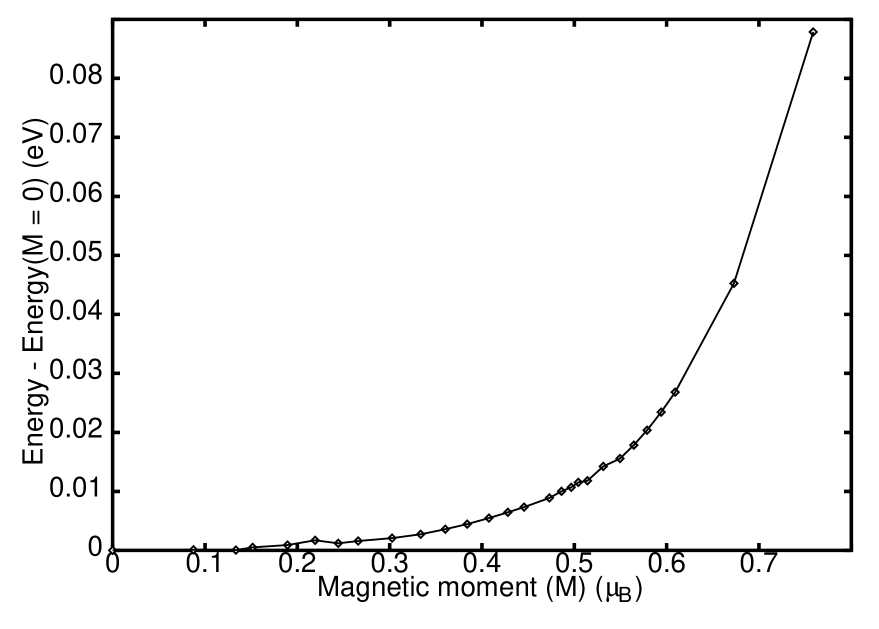
FIG. 1.: Calculated LSDA total energy, E, (in eV) with respect to M = 0$\mu_{B}$ as a function of calculated magnetic moment, M (in $\mu_{B}$).

FIG. 2.: Applied external magnetic field, H, (in Tesla) as a function of the calculated LSDA magnetic moment, M (in $\mu_{B}$). The total moment is shown together with spin component and the orbital component.

FIG. 3.: The external magnetic field, H, (in Tesla) as a function of the calculated magnetic moments, M (in $\mu_{B}$). The fit is to n $\leq$ 3 in Eqn. 2

FIG. 4.: Magnetic susceptibility, $\chi$, (in states/eV-cell) calculated from the fit of H, $\chi$ = $(\frac{\partial H}{\partial M})^{-1}$, shown as a function of M. The dashed line at 21 states/eV-cell corresponds to the experimental value of $\chi$ for Pd[30, 31].

FIG. 5.: Magnetic susceptibility, $\chi$, (in states/eV-cell) calculated from the fit of H, $\chi$ = $(\frac{\partial H}{\partial M})^{-1}$, shown as a function of H. The dashed line at 21 states/eV-cell corresponds to the experimental value of $\chi$ for Pd[30, 31].

FIG. 6.: $\frac{d\left\langle N(E_{F})v_{x}^{2}\right\rangle}{dE_{F}}$ as a function of energy, calculated by the bootstrap method. Note the numerical noise of up to 10%. Inset: $\left\langle N(E_{F})v_{x}^{2}\right\rangle$.

REFERENCES

- [1] C. Pfleiderer, M. Uhlarz, S.M. Hayden, R. Vollmer, H. von Lohneysen, N.R. Bernhoeft, and G.G. Lonzarich, Nature 412, 58 (2001).
- [2] S.S. Saxena, P. Agarwal, K. Ahilan, F.M. Grosche, R.K.W. Haselwimmer, M.J. Steiner, E. Pugh, I.R. Walker, S.R. Julian, P. Monthoux, G.G. Lonzarich, A. Huxley, I. Sheikin, D. Braithwaite, and J. Flouquet, Nature 406, 587 (2000).
- [3] D. Aoki, A. Huxley, E. Ressouche, D. Braithwaite, J. Flouquet, J.P Brison, E. Lhotel, and C. Paulsen, Nature 413, 613 (2001).
- [4] S.A. Grigera, R.S. Perry, A.J. Schofield, M. Chiao, S.R. Julian, G.G. Lonzarich, S.I. Ikeda, Y. Maeno, A.J. Millis, and A.P. Mackenzie, Science 294, 329 (2001).
- [5] K. Shimizu, T. Kimura, S. Furomoto, K. Takeda, K. Konati, Y. Onuki, and K. Amaya, Nature 412, 316 (2001).
- [6] A. Aguayo and D.J. Singh, Phys. Rev. B 66, 020401 (2002).
- [7] D.J. Singh and I.I. Mazin, Phys. Rev. B63, 165101 (2001).
- [8] D.J. Singh, Phys. Rev. B 61, 13397 (2000).
- [9] D.J. Singh and I.I. Mazin, Phys. Rev. Lett. 88, 187004 (2002).
- [10] B. I. Min, T. Oguchi, H. F. Jansen, and A. J. Freeman, J. Magn. Magn. Mater. 54-57, 1091 (1986).
- [11] D. J. Singh, in Intermetallic Compounds: Principles and Practice, edited by J. H. Westbrook and R. L. Fleisher (Wiley, New York, 1967, Vol. 1), p. 127.
- [12] V. L. Moruzzi and P. M. Marcus, Phys. Rev. B 47, 7878 (1993).
- [13] Li-Shing Hsu, Y.-K. Wang, and G. Y. Guo, J. Appl. Phys. 92, 1419 (2002).
- [14] D. Fay and J. Appel, Phys. Rev. B 16, 2325 (1977).
- [15] T. Jarlborg and A.J. Freeman, Phys. Rev. B 23, 3577 (1981).
- [16] A. Oswald, R. Zeller, and P.H. Dederichs, Phys. Rev. Lett. 56, 1419 (1986).
- [17] D.J. Singh and J. Ashkenazi, Phys. Rev. B 46 11570 (1992).
- [18] A. P. Murani, A. Tari and B. R. Coles, J. Phys. F: Met. Phys. 4, 1769 (1974).
- [19] D. Singh, Planewaves, Pseudopotentials, and the LAPW Method (Kluwer Academic, Boston, 1994).
- [20] P. Hohenberg and W. Kohn, Phys. Rev. 136, B864 (1964); W. Kohn and L. Sham, , 140, A1133 (1965).
- [21] J.P. Perdew and Y. Wang, Phys. Rev. B 45, 13244 (1996).
- [22] J.P. Perdew, K. Burke, and M. Ernzerhof, Phys. Rev. Lett. 77, 3865 (1996).
- [23] P. Blaha, K. Schwarz, G.K.H. Madsen, K. Kvasnicka, and J. Luitz, WIEN2k, An Augmented Plane Wave + Local Orbitals Program for Calculating Crystal Properties (Karlheinz Schwarz, Techn. Universitat Wien, Austria), 2001. ISBN 3-9501031-1-2
- [24] D. Singh, Phys. Rev. B 43, 6388 (1991).
- [25] D.D. Koelling and B. Harmon, J. Phys. C 10, 3107 (1977); P. Novak (unpublished).
- [26] J. Kunes, P. Novak, R. Schmid, P. Blaha, and K. Schwarz, Phys. Rev. B 64, 153102 (2001).
- [27] R.W.G. Wyckoff, Crystal Structures (Krieger, Melbourne, FL, 1986) Vol. 2.
- [28] M. Richter, P.M. Oppeneer, H. Eschrig, and B. Johansson, Phys. Rev. B 46, 13919 (1992).
- [29] P. Novak and J. Kuriplach, IEEE Trans. Magn. MAG-30, 1036 (1994).
- [30] S. Foner and E.J. McNiff, Phys. Rev. Lett. 19, 1438 (1967).
- [31] A. Tal, L.W. Roeland, M. Springford, P. Wise and R.G. Jordan, J. Phys. F: Met. Phys. 16, 893 (1986).
- [32] M. Shimizu, Rep. Prog. Phys. 44, 329 (1981).
- [33] T. Moriya, Spin fluctuations in itinerant electron magnetism (Berlin, Springer, 1985).
- [34] A.Z. Solontsov and D. Wagner, Phys. Rev. B51, 12410 (1995).
- [35] S.N. Kaul, J. Phys. Cond. Mat. 11, 7597 (1999).
- [36] A. Ishigaki and T. Moriya, J. Phys. Soc. Jpn. 67, 3924 (1998).
- [37] Despite close similarity, what we propose is not exactly the same as the formalism developed in Refs.[33, 34, 35] and others. The latter starts from a Landau functional which does not include any fluctuations at all, while we start from LDA energies which includes some, but not all fluctuations (if we had used the exact Hohenberg-Kohn theory we would not need any correction at all). Therefore entering Eq. 9 formally is not the experimental susceptibility as in the above-mentioned works.
- [38] I.I. Mazin, Phys. Rev. Lett. 83, 1427 (1999).
- [39] A. G. Petukhov, I. I. Mazin, L. Chioncel, and A. I. Lichtenstein, Phys. Rev. B 67 (15), 153106 (2003).
- [40] We have not performed GGA calculations at the same level of accuracy as LDA ones; however, GGA fixed spin moment calculations without the spin-orbit interaction indicate that correcting the spin susceptibility to the experimental value would require , larger but comparable with the value of 0.16 calculated above. Obviously, while neither LDA nor GGA cannot properly account for the long-range critical fluctuations, the question which approximation describes the non-critical physics better is open. In fact, the same question often arises in more standard band structure calculations as well.
- [41] B. Efron and R.J. Tibshirani, An Introduction to the Bootstrap, (Chapman & Hall, 1993).
- [42] Fermi velocity in Pd is renormalized by electron-paramagnon interaction in much the same way as by electron-phonon interaction. It is not entirely clear whether this renormalization should be taken into account when applying the fluctuation-dissipation theorem. Fortunately, this renormalization is not large enough to change the results in any important way; indeed, standard LDA calculations for optical conductivity, including plasma frequency, agree well with the experiment (see, e.g., Ref. [43]). Calculated DC transport agrees with the experiment within 15% [44]. The linear specific heat coefficient, usually the most affected quantity, also deviates from the calculated value of 8.2 mJ/mol K2 (using our and electron-phonon coupling constant of 0.35 from Ref. [44]) by less than 15% (using the experimental value of 9.42 mJ/mol K2 [45]).
- [43] E.G. Maksimov, I.I. Mazin, S.N.Rashkeev, Y.A. Uspenski, J. Phys. F: Met. Phys. 18, 833 (1988).
- [44] S.Y.Savrasov and D.Y.Savrasov, Phys. Rev. B 54, 16847 (1996).
- [45] B.W. Veal and J. A. Rayne, Phys. Rev. A: Gen. Phys. 135, A442 (1964).