Magnetic properties of the $S=1/2$ distorted diamond chain at $T=0$

Abstract

We explore, at $T=0$, the magnetic properties of the $S=1/2$ antiferromagnetic distorted diamond chain described by the Hamiltonian ${\cal H}=\sum_{j=1}^{N/3}\left\{J_{1}\left({\bi S}_{3j-1}\cdot{\bi S}_{3j}+{\bi S}_{3j}\cdot{\bi S}_{3j+1}\right)+J_{2}{\bi S}_{3j+1}\cdot{\bi S}_{3j+2}+J_{3}\left({\bi S}_{3j-2}\cdot{\bi S}_{3j}+{\bi S}_{3j}\cdot{\bi S}_{3j+2}\right)\right\}\allowbreak-H\sum_{l=1}^{N}S_{l}^{z}$ with $J_{1},\;J_{2},\;J_{3}\geq 0$, which well models ${\rm A_{3}Cu_{3}(PO_{4})_{4}}$ with ${\rm A=Ca,\,Sr}$, ${\rm Bi_{4}Cu_{3}V_{2}O_{14}}$ and azurite $\rm Cu_{3}(OH)_{2}(CO_{3})_{2}$. We employ the physical consideration, the degenerate perturbation theory, the level spectroscopy analysis of the numerical diagonalization data obtained by the Lanczos method and also the density matrix renormalization group (DMRG) method. We investigate the mechanisms of the magnetization plateaux at $M=M_{\rm s}/3$ and $M=(2/3)M_{\rm s}$, and also show the precise phase diagrams on the $(J_{2}/J_{1},\;J_{3}/J_{1})$ plane concerning with these magnetization plateaux, where $M=\sum_{l=1}^{N}S_{l}^{z}$ and $M_{\rm s}$ is the saturation magnetization. We also calculate the magnetization curves and the magnetization phase diagrams by means of the DMRG method.

1 Introduction

Low-dimensional quantum spin systems have attracted increasing attention in recent years. A few years ago, Ishii, Tanaka, Mori, Uekusa, Ohashi, Tatani, Narumi and Kindo [1] have reported the experimental results on a trimerized $S=1/2$ quantum spin chain $\rm Cu_{3}Cl_{6}(H_{2}O)_{2}\cdot 2H_{8}C_{4}SO_{2}$. From the structure-analysis experiment they have proposed a model shown in figure 1 for this substance [1]. The Hamiltonian of this model is written as

$${\cal H}={\cal H}_{0}+{\cal H}_{\rm Z}$$ (1)

$${\cal H}_{0}=J_{1}\sum_{j=1}^{N/3}\left({\bi S}_{3j-1}\cdot{\bi S}_{3j}+{\bi S}_{3j}\cdot{\bi S}_{3j+1}\right)+J_{2}\sum_{j=1}^{N/3}{\bi S}_{3j+1}\cdot{\bi S}_{3j+2}$$

$$~{}~{}~{}~{}~{}~{}~{}~{}~{}~{}~{}+J_{3}\sum_{j=1}^{N/3}\left({\bi S}_{3j-2}\cdot{\bi S}_{3j}+{\bi S}_{3j}\cdot{\bi S}_{3j+2}\right)$$ (2)

$${\cal H}_{\rm Z}=-H\sum_{l=1}^{N}S_{l}^{z}.$$ (3)

where ${\bi S}_{l}$ is the $S=1/2$ operator at the $l$th site and $N$ is the total number of spins in the system. All the coupling constants, $J_{1}$, $J_{2}$ and $J_{3}$, are supposed to be positive (antiferromagnetic). Hereafter we set $\tilde{J}_{2}\equiv J_{2}/J_{1}$ and $\tilde{J}_{3}\equiv J_{3}/J_{1}$. The magnetic field is denoted by $H$. We can assume $J_{1}\geq J_{3}$ without loss of generality because the $J_{1}<J_{3}$ case is equivalent to the $J_{1}>J_{3}$ case by interchanging the role of $J_{1}$ and $J_{3}$.

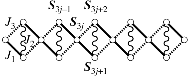
Figure 1: Sketch of the distorted diamond (DD) chain. Solid lines denote the coupling $J_{1}$, wavy lines the coupling $J_{2}$, and dotted lines the coupling $J_{3}$. We can assume $J_{1}\geq J_{3}$ without loss of generality.

This model has been named the “distorted diamond (DD) chain model”[2]. The name “diamond” comes from the mark of the playing cards, and “distorted” from the fact $J_{1}\neq J_{3}$ in general. The symmetric case ($J_{1}=J_{3}$) has first been proposed by Takano, Kubo and Sakamoto (TKS) [3] earlier than Ishii et al. [1] and ourselves [2]. We [2] have investigated the ground state properties of the $S=1/2$ DD chain model when $H=0$ by an analytical method as well as the level spectroscopy (LS) analysis of the numerical diagonalization data obtained by the Lanczos technique. Later the theoretical studies on the $S=1/2$ DD chain have also been reported by ourselves [4, 5], Sano and Takano [6] and Honecker and Läuchli [7].

Unfortunately the substance which was thought to be $\rm Cu_{3}Cl_{6}(H_{2}O)_{2}\cdot 2H_{8}C_{4}SO_{2}$ at first [1] has been proved to be $\rm Cu_{2}Cl_{4}\cdot H_{8}C_{4}SO_{2}$, the lattice of which is the two-leg zig-zag chain with the bond-alternation by the same group [8]. Now, however, the $S=1/2$ DD chain model is again in spotlight as a model for ${\rm A_{3}Cu_{3}(PO_{4})_{4}}$ with ${\rm A=Ca,\,Sr}$ [9, 10, 11], ${\rm Bi_{4}Cu_{3}V_{2}O_{14}}$ [12] and azurite $\rm Cu_{3}(OH)_{2}(CO_{3})_{2}$.

For ${\rm A_{3}Cu_{3}(PO_{4})_{4}}$ with ${\rm A=Ca,\,Sr}$, Drillon et al. [9, 10] measured the magnetic susceptibility $\chi(T)$, the specific heat $C(T)$ and the magnetization process $M(H)$, and proposed the model without $J_{2}$ interactions. Ajiro et al. [11] performed the high field magnetization process measurement up to 40T and the neutron diffraction experiment, and proposed the model with $J_{2}$ interactions. In these reports, a wide magnetization plateau at $M=M_{\rm s}/3$ was observed, where $M$ is the $z$ component of the total spin, defined by $M=\sum_{l=1}^{N}S_{l}^{z}$, and $M_{\rm s}$ is the saturation magnetization. The behavior of $\chi(T)$ and neutron diffraction results suggest that these substances are ferrimagnetic above the three-dimensional ordering temperature.

Sakurai et al. [12] reported $\chi(T)$, $M(H)$ (up to 28T), $C(T)$ and the ${\rm{}^{51}V}$ NMR of ${\rm Bi_{4}Cu_{3}V_{2}O_{14}}$. Unfortunately, they could not obtain any conclusion on the existence of the $M=M_{\rm s}/3$ plateau because $M\sim 0.27M_{\rm s}$ even when $H=28\,{\rm T}$. The ferrimagnetic behavior was not seen in $\chi(T)$ above the three-dimensional ordering temperature. It seems that this substance has the spin-fluid (SF) ground state above the three-dimensional ordering temperature.

Very recently, Kikuchi and co-workers [13, 14, 15] have reported the experimental results on the magnetic and thermal properties of azurite $\rm Cu_{3}(OH)_{2}(CO_{3})_{2}$. Following their reports, azurite has the spin-fluid (SF) ground state and the wide magnetization plateau at $M=M_{\rm s}/3$.

Thus, above the three-dimensional ordering temperature, the ground states of ${\rm A_{3}Cu_{3}(PO_{4})_{4}}$ with ${\rm A=Ca,\,Sr}$ seem to be ferrimagnetic, whereas those of ${\rm Bi_{4}Cu_{3}V_{2}O_{14}}$ and azurite $\rm Cu_{3}(OH)_{2}(CO_{3})_{2}$ seem to be SF. In view of these situations, we think it is very important to investigate the magnetic properties of the $S=1/2$ DD chain model in more detail. Throughout this paper we consider the $T=0$ case.

This paper is organized as follows. The ground-state properties at zero magnetic field are reviewed in §2. The magnetization plateaux at $M=M_{\rm s}/3$ and $M=(2/3)M_{\rm s}$ are discussed in §3 and §4, respectively. The numerical results for the magnetization curves and the magnetization phase diagram are presented in §5. The last section §6 is devoted to discussion and summary.

2 Review of the ground-state properties at zero magnetic field

Discussions presented in this section are confined to the case where $H=0$. We [2] have investigated the ground state of the $S=1/2$ DD chain model by an analytical method as well as the LS analysis of the numerical diagonalization data obtained by the Lanczos technique, and obtained the phase diagram shown in figure 2. There are three phases in this phase diagram; the ferrimagnetic (FRI) phase, the dimer (D) phase and the spin-fluid (SF) phase. The magnitude $S_{\rm tot}$ of the total spin ${\bi S}_{\rm tot}$, defined by ${\bi S}_{\rm tot}\equiv\sum_{l=1}^{N}{\bi S}_{l}$ and ${\bi S}_{\rm tot}^{2}=S_{\rm tot}(S_{\rm tot}+1)$, is $S_{\rm tot}=N/6$ in the FRI phase, whereas $S_{\rm tot}=0$ in the D and SF phases. In the D phase, there is a finite energy gap between the doubly degenerate ground state and the first excited state, while in the SF phase there is no energy gap.

Figure 2: Zero field ground state phase diagram of the $S=1/2$ DD chain model. The $\tilde{J}_{3}=1$ case is reduced to the model of TKS [3]. There are three phase in this phase diagram; the ferrimagnetic (FRI) phase, the dimer (D) phase and the spin-fluid (SF) phase.

When $J_{2}=0$, we can readily know that the ground state is the FRI state with $S_{\rm tot}=N/6$ by use of the Lieb-Mattis theorem [16]. The physical pictures of the FRI state are shown in figure 3, where the picture (a) holds good for the $J_{1}\sim J_{3}$ case, whereas (b) for the $J_{1}\gg J_{2},\;J_{3}$ case. The ellipses in (b) denote the effective 3-spin cluster which is formed when the interaction $J_{1}$ is much larger than the interactions $J_{2}$ and $J_{3}$. We represent the $S_{l}^{z}=1/2$ and $S_{l}^{z}=-1/2$ states of the $l$th single spin by $\uparrow_{l}$ and $\downarrow_{l}$, respectively. Then, the ground state wave functions of the $j$th cluster in the case of $J_{2}=J_{3}=0$ are expressed as

$$\phi_{1,j}={1\over\sqrt{6}}\left(|\uparrow_{3j-1}\uparrow_{3j}\downarrow_{3j+1}\rangle-2|\uparrow_{3j-1}\downarrow_{3j}\uparrow_{3j+1}\rangle+|\downarrow_{3j-1}\uparrow_{3j}\uparrow_{3j+1}\rangle\right)$$ (4)

and

$$\phi_{2,j}={1\over\sqrt{6}}\left(|\downarrow_{3j-1}\downarrow_{3j}\uparrow_{3j+1}\rangle-2|\downarrow_{3j-1}\uparrow_{3j}\downarrow_{3j+1}\rangle+|\uparrow_{3j-1}\downarrow_{3j}\downarrow_{3j+1}\rangle\right)$$ (5)

for $S_{\rm tot}^{(3)z}=1/2$ and $S_{\rm tot}^{(3)z}=-1/2$, respectively, where $S_{\rm tot}^{(3)z}$ is the $z$ component of the total spin of the 3-spin cluster. When all the 3-spin clusters are effectively in the $\phi_{1}$ (or $\phi_{2}$) state, the FRI state shown by figure 3(b) is realized. This physical consideration has been developed in [4, 7] by use of the degenerate perturbation theory [17] around the point $\tilde{J}_{2}=\tilde{J}_{3}=0$. In fact, the quantum phase transition between the FRI and SF phases takes place at $\tilde{J}_{3}=\tilde{J}_{2}$ near $(\tilde{J}_{2},\tilde{J}_{3})=(0,0)$, and it is of the first order. This shows very good agreement with the numerical results (see figure 2). The quantum phase transition between the FRI and D phases is also of the first order.

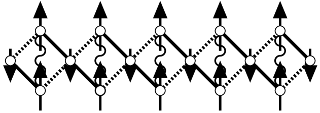
(a)     (b)

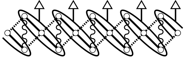
Figure 3: Physical pictures of the FRI ground state for the $S=1/2$ DD chain model. Open ellipses with open triangles in (b) denote the 3-spin clusters in the state $\phi_{1}$.

In the case of $J_{3}=0$, our DD chain is reduced to the $J_{1}$-$J_{1}$-$J_{2}$ trimerized antiferromagnetic chain, the ground state of which is the SF state. In particular, in the case of $J_{1}=J_{2}$, it is further simplified to the uniform antiferromagnetic chain.

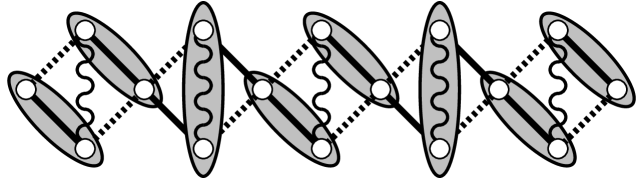
(a)     (b)

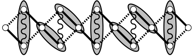
Figure 4: Physical pictures of the D ground state for the $S=1/2$ DD chain model. Two spins in a shadowed ellipse effectively form a singlet dimer pair.

The D phase is caused by the frustration, and is doubly degenerate due to the spontaneous breaking of the translational symmetry (SBTS), as shown in figure 4. The D phase is realized in the region where the frustration effect seems to be severe. We note that there is no frustration when $J_{2}=0$ or $J_{3}=0$. The quantum phase transition between the SF and D phases is essentially the same as that in the $S=1/2$ chain with next-nearest-neighbor interactions [18, 19], and is of the Berezinskii-Kosterlitz-Thouless (BKT) type [20, 21], as has been fully discussed in our previous paper [2].

                 (a)

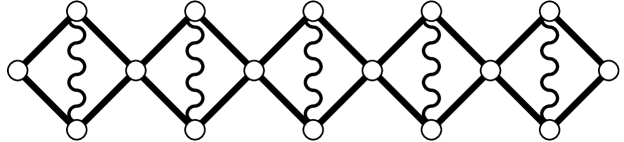
                 (b)

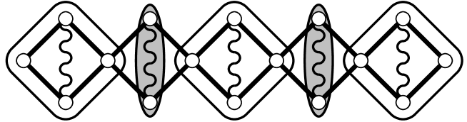
                 (c)

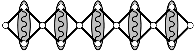
Figure 5: (a) The model of Takano, Kubo and Sakamoto [3]. (b) The tetramer-dimer (TD) state, where the rectangles represent tetramers and the ellipses singlet dimers. (c) The dimer-monomer (DM) state.

As we have mentioned in §1, the symmetric case $J_{1}=J_{3}$, which is shown in figure 5(a), has first been proposed by TKS [3]. They have found that the ground state is the FRI state, the tetramer-dimer (TD) state or the dimer-monomer (DM) state, depending on whether $\tilde{J}_{2}<0.909$, $0.909<\tilde{J}_{2}<2$ or $2<\tilde{J}_{2}$. The value $0.909$ of the FRI-TD boundary has been calculated by the numerical method, whereas the value $2$ of the TD-DM boundary is the exact one obtained by an analytical method. In the TD state, as shown in figure 5(b), four spins of the diamond unit ${\bi S}_{3j-3}$, ${\bi S}_{3j-2}$, ${\bi S}_{3j-1}$ and ${\bi S}_{3j}$ (or ${\bi S}_{3j}$, ${\bi S}_{3j+1}$, ${\bi S}_{3j+2}$ and ${\bi S}_{3j+3}$) form a tetramer, and two spins ${\bi S}_{3j+1}$ and ${\bi S}_{3j+2}$ (or ${\bi S}_{3j+4}$ and ${\bi S}_{3j+5}$) form a singlet dimer. Obviously, the TD state is doubly degenerate due to the SBTS. In the DM state, on the other hand, two spins ${\bi S}_{3j+1}$ and ${\bi S}_{3j+2}$, connected by the $J_{2}$ interactions, form a singlet dimer and the remaining joint spins ${\bi S}_{3j}$ are completely free, as shown in figure 5(c). Thus, the DM state is $2^{N/3}$-fold degenerate. It is very interesting that the ground state can be exactly expressed as the direct product of the local states in a finite range of the parameter region $\tilde{J}_{2}>0.909$.

The TD state is very peculiar to the $J_{1}=J_{3}$ case. Namely, if $J_{1}>J_{3}$, the tetramer which consists of ${\bi S}_{3j-3}$, ${\bi S}_{3j-2}$, ${\bi S}_{3j-1}$ and ${\bi S}_{3j}$ is effectively decomposed into two dimers, the $({\bi S}_{3j-3}$, ${\bi S}_{3j-2})$ pair and the $({\bi S}_{3j-1}$, ${\bi S}_{3j})$ pair. Two spins in each pair are connected by the $J_{1}$ interaction which is larger than the $J_{3}$ one. This decomposition leads to the doubly degenerate D state shown in figure 4. Thus, the TD state is the special case of the doubly degenerate D state.

The $2^{N/3}$-fold degeneracy of the DM state is lifted when $J_{1}\neq J_{3}$. In other words, the effective interaction between the free spins ${\bi S}_{3j}$ and ${\bi S}_{3(j+1)}$ appears through the dimer located between them. Honecker and Läuchli [7] have derived the effective interaction between ${\bi S}_{3j}$ and ${\bi S}_{3(j+1)}$ as

$$J_{\rm eff}={(J_{1}-J_{3})^{2}\over J_{2}}\left({1\over 2}+\cdots\right)$$ (6)

which leads to the SF ground state. The effective interaction $J_{\rm eff}$ vanishes when $J_{1}=J_{3}$, which is consistent with TKS’s result [3] on the DM state. Then, the DM state is also peculiar to the $J_{1}=J_{3}$ case and is the special case of the SF state.

3 Magnetization plateau at $M=M_{\rm s}/3$

In this section, we discuss the magnetization plateau at $M=M_{\rm s}/3$. Since the Hamiltonian has the trimer nature, as is shown in figure 6, the mechanism for the $M=M_{\rm s}/3$ plateau is just the same as that for the trimerized chain (Figure 7) investigated by Okamoto and Kitazawa [22] and by Honecker [23]. The $M=M_{\rm s}/3$ plateau can be realized without any SBTS. This is consistent with the necessary condition for the magnetization plateau by Oshikawa, Yamanaka and Affleck (OYA) [24],

$$n(S-\langle m\rangle)={\rm integer}$$ (7)

where $n$ is the periodicity of the wave function of the plateau state, $S$ the magnitude of spins and $\langle m\rangle$ the average magnetization per one spin in the plateau.

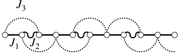
Figure 6: Single chain representation of the DD chain model.

Figure 7: Antiferromagnetic chain with the trimerization.

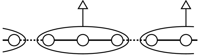
(a)     (b)

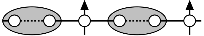
Figure 8: Two mechanisms for the $M=M_{\rm s}/3$ plateau for the $S=1/2$ trimerized chain: (a) the plateau A and (b) the plateau B. Open ellipses denote the trimers with $S^{(3)z}_{\rm tot}=1/2$ and shaded ellipses denote the singlet dimers

Here we explain the mechanism for the $M=M_{\rm s}/3$ plateau of the $S=1/2$ trimerized chain. When $0<J\ll J^{\prime}$, each of three spins connected by $J^{\prime}$ forms an effective trimer with $S^{(3)z}_{\rm tot}=1/2$ (or $-1/2$), the wave function of which is $\phi_{1}$ (or $\phi_{2}$). When the magnetic field is applied, all the trimers belong to the $S^{(3)z}_{\rm tot}=1/2$ state, which brings about $M=M_{\rm s}/3$, as shown in figure 8(a). The plateau due to this mechanism is named the “plateau A”. The mechanism of the plateau A state is essentially the same as that of the FRI state for the $J_{1}\gg J_{2},\;J_{3}$ case when $H=0$, which is already explained in §2. When $J\gg J^{\prime}>0$, on the other hand, each pair of two spins connected by $J$ forms an effective singlet dimer pair and the remaining spins are nearly free. When the magnetic field is applied, the nearly free spins turn to the direction of the field, resulting also in $M=M_{\rm s}/3$, as shown in figure 8(b). We call the plateau due to this mechanism the “plateau B”. Thus, there are two mechanisms for the $M=M_{\rm s}/3$ plateau. It is easily seen that the change of the plateau mechanism occurs at $J=J^{\prime}$, where the trimerized chain is reduced to the uniform chain having no gap (i.e., no plateau) in the excitation spectrum. This situation is most simply seen in the trimerized $XY$ chain [25] which is exactly solvable.

(a) (b)

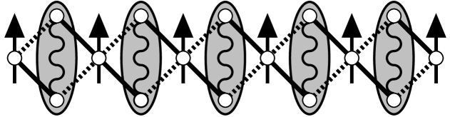
Figure 9: Two mechanisms for the $M=M_{\rm s}/3$ plateau for the $S=1/2$ DD chain: (a) the plateau A and (b) the plateau B. Shaded ellipses denote the singlet dimers and open ellipses denote the trimers with $S_{\rm tot}^{(3)z}=1/2$.

A similar situation is expected to hold for the present $S=1/2$ DD chain model. The pictures of the plateaux A and B are depicted in figure 9(a) and (b), respectively, by use of the diamond form. When $J_{3}=0$, our model is reduced to the simple trimerized chain discussed above. Then, the change of the plateau mechanism occurs at $J_{1}=J_{2}$ when $J_{3}=0$. To find the phase boundary between the plateaux A and B for the general case, we have to rely on the numerical method. One of the most powerful methods is the level spectroscopy (LS) [26, 27]. Kitazawa [28] has developed the LS for this kind of transition (belonging to the Gaussian universality class) by use of the twisted boundary condition (TBC) instead of the periodic boundary condition (PBC). This method has been applied to several magnetization plateau problems in a successful way [22, 29, 30, 31].

In finite size systems with the PBC, the $M=M_{\rm s}/3$ plateau state changes smoothly from the plateau A state to the plateau B state when the parameter $J_{2}/J_{1}$ runs from 0 to $\infty$, although the plateau width takes the smallest value at the transition point. Under the TBC

$${\bi S}_{N}\cdot{\bi S}_{1}\Rightarrow-S_{N}^{x}S_{1}^{x}-S_{N}^{y}S_{1}^{y}+S_{N}^{z}S_{1}^{z},$$ (8)

on the other hand, the plateau A state and the plateau B state can be easily distinguished even in finite size systems by the eigenvalue $P$ of the space inversion operator

$${\bi S}_{j}\Rightarrow{\bi S}_{N-j+1}.$$ (9)

Since it is believed that the boundary condition does not affect any physical quantities in the $N\to\infty$ limit, we distinguish the ground state by comparing the lowest energies with $P=\pm 1$. In other words, we can find the phase boundary between the plateaux A and B from the crossing of the lowest energies with $P=\pm 1$ as functions of the quantum parameters in the Hamiltonian. This is the physical interpretation of Kitazawa’s TBC method [28]. He [28] has consolidated the foundations of his TBC method by use of the bosonization, the renormalization group method and the conformal field theory.

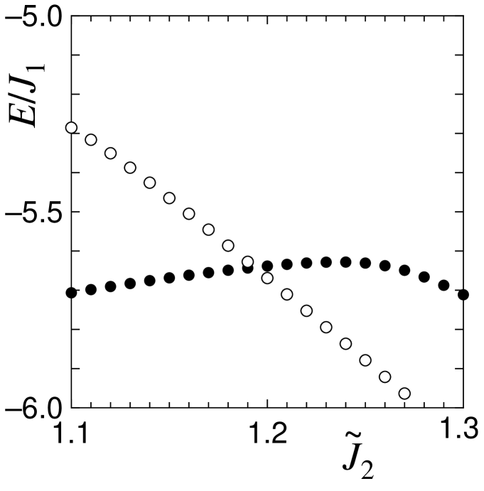
Figure 10: Crossing of the lowest energies in the $M=M_{\rm s}/3$ sector with $P=1$ (closed circles) and $P=-1$ (open circles) for the $N=18$ and $\tilde{J}_{3}=0.55$ case under the TBC, when $\tilde{J}_{2}$ is run. The crossing point of these two curves locates at $\tilde{J}_{2}\simeq 1.193$.

Figure 10 shows the crossing of the lowest energies with $P=\pm 1$ when $N=18$ and $\tilde{J}_{3}=0.55$. We can see that two curves cross with each other at $\tilde{J}_{2}^{\rm(cr)}(18)\simeq 1.193$, close to which the quantum transition point $\tilde{J}_{2}^{\rm(cr)}$ between the plateau A and B phases for the $N\to\infty$ system is expected to be located. An accurate value of $\tilde{J}_{2}^{\rm(cr)}$ may be estimated by extrapolating $\tilde{J}_{2}^{\rm(cr)}(N)$ to the $N\to\infty$ limit. Performing this extrapolation we have assumed an $N$ dependence of $\tilde{J}_{2}^{\rm(cr)}(N)$ as

$$\tilde{J}_{2}^{\rm(cr)}(N)=\tilde{J}_{2}^{\rm(cr)}+c_{1}/N^{2}+c_{2}/N^{4}$$ (10)

where $c_{1}$ and $c_{2}$ are numerical constants, and have employed the finite size values, $\tilde{J}_{2}^{\rm(cr)}(12)$, $\tilde{J}_{2}^{\rm(cr)}(18)$ and $\tilde{J}_{2}^{\rm(cr)}(24)$. Repeating this procedure with sweeping $\tilde{J}_{3}$, we have obtained the $M=M_{\rm s}/3$ plateau phase diagram shown in figure 11. The estimated value of errors of the phase boundary is, for instance, $\tilde{J}_{2}^{\rm(cr)}=1.193\pm 0.001$ (or better) for $\tilde{J}_{3}=0.55$.

Figure 11: $M=M_{\rm s}/3$ plateau phase diagram of the $S=1/2$ DD chain model.

Figure 12: Normalized $M=M_{\rm s}/3$ plateau width $W_{(1/3)}/H_{\rm s}$ as a function of $\tilde{J}_{2}$ when $\tilde{J}_{3}=0.55$, where $H_{\rm s}$ is the saturation field. The plateau width $W_{(1/3)}$ vanishes at $\tilde{J}_{3}\simeq 1.193$, which well agrees with the transition point between the plateaux A and B in figure 11. The cusp at $\tilde{J}_{3}\simeq 0.561$ corresponds to the FRI-SF transition in figure 2.

We have performed the density matrix renormalization group (DMRG) calculation [32, 33] to obtain the ground state magnetization curves and the magnetization phase diagrams for our $S=1/2$ DD chain model, the details of which will be described in §5. Here, we present in figure 12 the width $W_{(1/3)}$ (see equation (29) below) of the $M=M_{\rm s}/3$ plateau for $\tilde{J}_{3}=0.55$ in the $N\to\infty$ limit; in this figure $W_{(1/3)}$ is plotted as a function of $\tilde{J}_{2}$. The point where $W_{(1/3)}$ vanishes is the transition point ($\tilde{J}_{2}\simeq 1.193$), the result shown in figure 12 being in very good agreement with the above-mentioned result obtained by the LS method with the TBC. We see a cusp in the curve at $\tilde{J}_{2}\simeq 0.561$. This cusp corresponds to the FRI-SF transition in figure 2 (see also figure 19(b) below). In fact, an infinitesimal small field brings about the $M=M_{\rm s}/3$ magnetization state in the FRI region, whereas a finite field is required for the $M=M_{\rm s}/3$ magnetization state in the SF and D regions.

Figure 13: Behavior of $\langle S_{l}^{z}\rangle$ of the $N=96$ system (a) in the plateau A region, where $(\tilde{J}_{2},\;\tilde{J}_{3})=(0.80,\;0.55)$, and (b) in the plateau B region, where $(\tilde{J}_{2},\;\tilde{J}_{3})=(1.50,\;0.55)$.

Let us now discuss the expectation value $\langle S_{l}^{z}\rangle$ of each spin in the $M=M_{\rm s}/3$ plateau state. In the plateau A region, the approximate wave function of the $j$th 3-spin cluster is

$$\phi_{1,j}={1\over\sqrt{6}}\left(|\uparrow_{3j-1}\uparrow_{3j}\downarrow_{3j+1}\rangle-2|\uparrow_{3j-1}\downarrow_{3j}\uparrow_{3j+1}\rangle+|\downarrow_{3j-1}\uparrow_{3j}\uparrow_{3j+1}\rangle\right)$$ (11)

which leads to

$$\langle S_{3j-1}^{z}\rangle=\langle S_{3j+1}^{z}\rangle={1\over 3}~{}~{}~{}~{}~{}\langle S_{3j}\rangle=-{1\over 6}.$$ (12)

Thus, the expectation values $\langle S_{l}^{z}\rangle$ should be

$$\left\{\cdots,\left({1\over 3},-{1\over 6},{1\over 3}\right),\left({1\over 3},-{1\over 6},{1\over 3}\right),\left({1\over 3},-{1\over 6},{1\over 3}\right),\cdots\right\}$$ (13)

where three spins in a parenthesis form a 3-spin cluster. In the plateau B region, on the other hand, it is very easy to see that $\langle S_{l}^{z}\rangle$ should be

$$\left\{\cdots,\left(0,0\right),{1\over 2},\left(0,0\right),{1\over 2},\left(0,0\right),{1\over 2},\left(0,0\right),{1\over 2},\cdots\right\}$$ (14)

where two spins in a parenthesis form a singlet dimer. Figure 13 shows the DMRG result for $\langle S_{l}^{z}\rangle$ for the $N=96$ system in the plateau A region, where $(\tilde{J}_{2},\;\tilde{J}_{3})=(0.80,\;0.55)$, and that in the plateau B region, where $(\tilde{J}_{2},\;\tilde{J}_{3})=(1.50,\;0.55)$. Then, the behavior of $\langle S_{l}^{z}\rangle$ in this figure is quite consistent with our picture of the mechanisms for the $M=M_{\rm s}/3$ plateau.

4 Magnetization plateau at $M=(2/3)M_{\rm s}$

Our incipient discussions on the $M=(2/3)M_{\rm s}$ plateau of the $S=1/2$ DD chain model are given in a previous paper [5]; here we aim at discussing it in much more detail.

Since the unit cell of the present model consists of three $S=1/2$ spins, the OYA condition [24] tells us that if the SBTS does not occur, the possible magnetization plateau for $0<M<M_{\rm s}$ is only at $M=M_{\rm s}/3$. Thus, the SBTS is necessary for the realization of the $M=(2/3)M_{\rm s}$ plateau. In the 3-spin cluster limit where $\tilde{J}_{2}=\tilde{J}_{3}=0$, the $M=(2/3)M_{\rm s}$ magnetization state is realized when a half of the 3-spin clusters are in the $S_{\rm tot}^{(3)z}=1/2$ state and the remaining half are in the $S_{\rm tot}^{(3)z}=3/2$ state. The configuration of these two states are completely free when $\tilde{J}_{2}=\tilde{J}_{3}=0$, resulting in the $2^{N/3}$-fold degeneracy. This high degeneracy is lifted when we introduce $\tilde{J}_{2}$ and $\tilde{J}_{3}$.

Let us discuss the $M=(2/3)M_{\rm s}$ magnetization plateau problem based on the above picture by use of the degenerate perturbation theory [17]. The lowest energy state of the $j$th 3-spin cluster with $S_{\rm tot}^{(3)z}=1/2$ is given by

$$\psi_{1,j}={1\over\sqrt{6}}\left(|\uparrow_{3j-1}\uparrow_{3j}\downarrow_{3j+1}\rangle-2|\uparrow_{3j-1}\downarrow_{3j}\uparrow_{3j+1}\rangle+|\downarrow_{3j-1}\uparrow_{3j}\uparrow_{3j+1}\rangle\right)$$ (15)

which is nothing but equation (4). Here we use the symbol $\psi_{1,j}$ for convenience. The energy of this state is

$$E_{1}=-J_{1}-{1\over 2}H.$$ (16)

On the other hand, the state of the $j$th 3-spin cluster with $S_{\rm tot}^{(3)z}=3/2$ is

$$\psi_{2,j}=|\uparrow_{3j-1}\uparrow_{3j}\uparrow_{3j+1}\rangle$$ (17)

having the energy

$$E_{2}={1\over 2}J_{1}-{3\over 2}H.$$ (18)

Using the pseudo-spin operator ${\bi T_{j}}$, where ${\bi T_{j}}^{2}=T_{j}(T_{j}+1)$ with $T_{j}=1/2$, we express the $\psi_{1,j}$ and $\psi_{2,j}$ states by the $T_{j}^{z}=-1/2$ and $T_{j}^{z}=+1/2$ states, respectively. We neglect the other 6 states of the $j$th 3-spin cluster, which can be justified near $\tilde{J}_{2}=\tilde{J}_{3}=0$. We note that $E_{1}=E_{2}$ when the magnetic field is given by $H=H_{\rm 2/3}^{(0)}\equiv(3/2)J_{1}$. The lowest order perturbation calculation with respect to $\tilde{J}_{2}$ and $\tilde{J}_{3}$ leads to the effective Hamiltonian for the pseudo-spin operator ${\bi T_{j}}$

$${\cal H}_{\rm eff}=\sum_{j}\{J^{\perp}_{\rm eff}(T_{j}^{x}T_{j+1}^{x}+T_{j}^{y}T_{j+1}^{y})+J^{z}_{\rm eff}T_{j}^{z}T_{j+1}^{z}\}-H_{\rm eff}\sum_{j}T_{j}^{z}$$ (19)

where

$$J^{\perp}_{\rm eff}={J_{2}-4J_{3}\over 6}$$ (20)

$$J^{z}_{\rm eff}={J_{2}+8J_{3}\over 36}$$ (21)

$$H_{\rm eff}=H-H_{2/3}^{(0)}-{5J_{2}+22J_{3}\over 36}.$$ (22)

The ground state of the effective Hamiltonian (19) is either the Néel state or the SF state depending on whether $\Delta_{\rm eff}>1$ or $0\leq\Delta_{\rm eff}\leq 1$, where $\Delta_{\rm eff}$ is

$$\Delta_{\rm eff}\equiv{J^{z}_{\rm eff}\over|J^{\perp}_{\rm eff}|}={J_{2}+8J_{3}\over 6|J_{2}-4J_{3}|}.$$ (23)

Thus, the Néel ground state is realized when

$${5\over 32}<{J_{3}\over J_{2}}<{7\over 16}.$$ (24)

The Néel and SF ground states in the ${\bi T}$-picture correspond to the $M=(2/3)M_{\rm s}$ plateauful and plateauless states in the original ${\bi S}$-picture, respectively. The transition between the plateauful and plateauless states is of the BKT type [20, 21]. The magnetic field $H_{2/3}$ given by the solution of $H_{\rm eff}=0$, i.e.,

$$H_{2/3}\equiv H_{2/3}^{(0)}+{5J_{2}+22J_{3}\over 36}={54J_{1}+5J_{2}+22J_{3}\over 36}.$$ (25)

represents the magnetic field corresponding to the center of the magnetization plateau in the plateauful case, and that corresponding to the $M=M_{\rm s}/3$ magnetization in the plateauless case. This degenerate perturbation calculation has already been developed in [5, 7]. The physical picture of the $M=(2/3)M$ plateau is shown in figure 14.

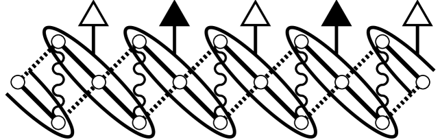
Figure 14: Physical picture of the $M=(2/3)M_{\rm s}$ plateau state for the $S=1/2$ DD chain model. Ellipses with open and closed triangles denote the 3-spin clusters with the $\psi_{1}$ and $\psi_{2}$ states, respectively.

For the purpose of drawing the $M=(2/3)M_{\rm s}$ plateau phase diagram, we have performed the numerical diagonalization of the finite size Hamiltonian by the Lanczos method. We can apply the LS method [19, 26, 27, 34, 35] to this kind of plateauful-plateauless transition of the BKT type [36, 37, 38, 39] accompanied by the SBTS. The plateauful-plateauless transition point can be obtained from the crossing point of $\Delta E_{0}(N,M=(2/3)M_{\rm s})$ and $\Delta E_{\pm 1}(N,M=(2/3)M_{\rm s})$ as functions of the quantum parameters. Here, $\Delta E_{0}(N,M)$ and $\Delta E_{\pm 1}(N,M)$ are defined, respectively, by

$$\Delta E_{0}(N,M)\equiv E_{1}\left(N,M\right)-E_{0}\left(N,M\right)$$ (26)

$$\Delta E_{\pm 1}(N,M)\equiv{1\over 2}\left\{E_{0}\left(N,M+1\right)+E_{0}\left(N,M-1\right)\right\}-E_{0}\left(N,M\right)$$ (27)

where $E_{0}(N,M)$ and $E_{1}(N,M)$ are, respectively, the lowest and second lowest energies in the subspace of the magnetization $M$ for the finite size system with $N$ spins. It is noted that the $M=(2/3)M_{\rm s}$ state is either plateauful (the Néel state in the ${\bi T}$-picture) or plateauless (the SF state in the ${\bi T}$-picture) depending on whether $\Delta E_{0}(N,M=(2/3)M_{\rm s})<\Delta E_{\pm 1}(N,M=(2/3)M_{\rm s})$ or $\Delta E_{0}(N,M=(2/3)M_{\rm s})>\Delta E_{\pm 1}(N,M=(2/3)M_{\rm s})$.

Figure 15: $\Delta E_{0}(N,M=(2/3)M_{\rm s})$ (closed circles) and $\Delta E_{\pm 1}(N,M=(2/3)M_{\rm s})$ (open circles) with $N=18$ ($M_{\rm s}=9$) as functions of $\tilde{J}_{3}$ when $\tilde{J}_{2}=0.80$. Approximated values for the plateauful-plateauless phase boundary points in the $N\to\infty$ limit are known from the crossings of $\Delta E_{0}(N,M=(2/3)M_{\rm s})$ and $\Delta E_{\pm 1}(N,M=(2/3)M_{\rm s})$. The point where $\Delta E_{0}(N,M=(2/3)M_{\rm s})$ vanishes ($\tilde{J}_{3}\simeq 0.25$; see the inset) corresponds to the Ising case of the pseudo-spin Hamiltonian (19).

Figure 15 shows the behaviors of $\Delta E_{0}(N,M=(2/3)M_{\rm s})$ and $\Delta E_{\pm 1}(N,M=(2/3)M_{\rm s})$ with $N=18$ ($M_{\rm s}=9$) as functions of $\tilde{J}_{3}$ when $\tilde{J}_{2}=0.80$. The value of $\tilde{J}_{3}$ at each crossing point is expected to be an approximate value for the plateauful-plateauless transition point $\tilde{J}_{3}^{\rm(cr)}$ in the $N\to\infty$ limit. We have carried out, to estimate $\tilde{J}_{3}^{\rm(cr)}$, an extrapolation to this limit similar to that in the case of the estimation of $\tilde{J}_{2}^{\rm(cr)}$ for the $M=M_{\rm s}/3$ plateau phase diagram, discussed in §3, and have obtained the $M=(2/3)M_{\rm s}$ plateau phase diagram depicted in figure 16. In this figure a good agreement is found between the numerical result and the analytical prediction given by equation (24) near $(\tilde{J}_{2},\tilde{J}_{3})=(0,0)$. We note that the point $\Delta E_{0}=0$ ($\tilde{J}_{3}\simeq 0.25$) corresponds to the Ising case ($J_{\rm eff}^{\perp}=0$) of the pseudo-spin Hamiltonian (19). The double degeneracy in the Néel ground state is realized only in the $N\to\infty$ limit in usual cases, whereas it is realized even in finite size systems for the Ising case. Thus, the point $\Delta E_{0}=0$, which means the doubly degenerate ground state, corresponds to the Ising case.

Figure 16: $M=(2/3)M_{\rm s}$ plateau phase diagram of the $S=1/2$ DD chain model. Closed circles denote the numerical results, and the dashed lines the results of the degenerate perturbation calculation given by equation (24).

The expectation value $\langle S_{l}^{z}\rangle$ of the $(2/3)M_{\rm s}$ plateau state can be obtained from the above-mentioned physical picture (figure 14); equations (15) and (17) yields for $\langle S_{l}^{z}\rangle$

$$\left\{\cdots,\overbrace{\left({1\over 3},-{1\over 6},{1\over 3}\right)}^{\displaystyle{\psi_{1}}},\overbrace{\left({1\over 2},{1\over 2},{1\over 2}\right)}^{\displaystyle{\psi_{2}}},\overbrace{\left({1\over 3},-{1\over 6},{1\over 3}\right)}^{\displaystyle{\psi_{1}}},\overbrace{\left({1\over 2},{1\over 2},{1\over 2}\right)}^{\displaystyle{\psi_{2}}},\cdots\right\}$$ (28)

where three spins in a parenthesis form a 3-spin cluster. Figure 17 shows the behaviors of $\langle S_{l}^{z}\rangle$ which are obtained by using the DMRG method for the $N=96$ system in the $(\tilde{J}_{2},\;\tilde{J}_{3})=(0.80,\;0.27)$ and $(\tilde{J}_{2},\;\tilde{J}_{3})=(0.80,\;0.30)$ cases. As can be readily seen, the behavior of $\langle S_{l}^{z}\rangle$ is quite consistent with equation (28). Of course, the ideal behavior given by this equation is expected in the $\Delta_{\rm eff}=\infty$ limit (the Ising limit) in the effective Hamiltonian (19), even if the mapping onto the ${\bi T}$-picture is justified. In the case where $\Delta_{\rm eff}$ is finite, the hybridization between the $\psi_{1}$ and $\psi_{2}$ states occurs, which well explains the fact that $\langle S_{3j}^{z}\rangle<\langle S_{3j-1}^{z}\rangle=\langle S_{3j+1}^{z}\rangle$ in the $\psi_{2}$-rich cluster. The behavior of $\langle S_{l}^{z}\rangle$ of the $\psi_{2}$-rich cluster in the $(\tilde{J}_{2},\;\tilde{J}_{3})=(0.80,\;0.27)$ case is nearer to the ideal behavior than that in the $(\tilde{J}_{2},\;\tilde{J}_{3})=(0.80,\;0.30)$ case. This suggests that the parameter set in the former case is nearer to the Ising limit of the effective Hamiltonian (19) than that in the latter case. In fact, the Ising limit is realized when $\tilde{J}_{3}\simeq 0.25$ for $\tilde{J}_{2}=0.55$, as can be seen from figure 15.

Figure 17: Behavior of $\langle S_{l}^{z}\rangle$ of the $N=96$ system in the $M=(2/3)M_{\rm s}$ plateau state, where (a) $(\tilde{J}_{2},\;\tilde{J}_{3})=(0.80,\;0.27)$ and (b) $(\tilde{J}_{2},\;\tilde{J}_{3})=(0.80,\;0.30)$

5 Magnetization curves and magnetization phase diagrams

In order to calculate the ground state magnetization curve of the present $S=1/2$ DD chain model, we have employed the DMRG method [32, 33]. The procedure of our DMRG calculation is briefly summarized in reference [4].

We have computed $E_{0}(N,M)$ for finite size systems with up to $N=96$ ($N=216$) spins for general (special) values of $\tilde{J}_{2}$ and $\tilde{J}_{3}$. Once the values of $E_{0}(N,M)$ for all nonnegative $M$’s ($M=0$, $1$, $2$, $\cdots$, $N/2$) are known, the ground state magnetization curve can be obtained by plotting as a function of $H$ the average magnetization $\langle m\rangle$ per one spin, where $\langle m\rangle$ is the value of $m$ which yields the minimum among $\{E_{0}(N,mN)/N-Hm\}$’s with $m=0$, $1/N$, $2/N$, $\cdots$, $1/2$. As is naturally expected, the resulting magnetization curve is a stepwisely increasing function of $H$. Following Bonner and Fisher’s pioneering work [40], we may obtain, except for plateau regions, a satisfactorily good approximation to the ground state magnetization curve in the $N\to\infty$ limit by drawing a smooth curve through the midpoints of the steps in the finite size results. As for the plateau regions, on the other hand, we can estimate the lowest and highest values of $H$ in the $N\to\infty$ limit, denoted by $H_{p,{\rm l}}$ and $H_{p,{\rm h}}$, respectively, giving the $M=pM_{\rm s}$ ($p=0$, $1/3$, $2/3$ or $1$) plateau by extrapolating the corresponding finite size values to this limit.

The magnetization curves in the $N\to\infty$ limit thus obtained for the $(\tilde{J}_{2},\;\tilde{J}_{3})=(0.80,\;0.27)$ case and the $(\tilde{J}_{2},\;\tilde{J}_{3})=(0.80,\;0.55)$ case are shown in figure 18. It is noted that $H_{p,{\rm l}}$ and $H_{p,{\rm h}}$ in both cases are estimated by fitting the finite size results for $N=48$, $72$ and $96$ to a quadratic function of $1/N^{2}$, which is similar to equation (10). The $H=0$ ground state phase in the former case is the SF phase (see figure 2), and therefore we have no $M=0$ plateau. Since that in the latter case is the D phase, on the other hand, we have in principle a finite $M=0$ plateau, although the $M=0$ plateau width is so narrow that we cannot see it clearly (see figure 19(b) below). The wide $M=M_{\rm s}/3$ plateaux are found in both cases, while the $M=(2/3)M_{\rm s}$ plateau is observed only in the former case, which is consistent with the $M=(2/3)M_{\rm s}$ plateau phase diagram shown in figure 16.

Figure 18: Magnetization curves in the $N\to\infty$ limit for (a) $(\tilde{J}_{2},\;\tilde{J}_{3})=(0.80,0.27)$ and (b) $(\tilde{J}_{2},\;\tilde{J}_{3})=(0.80,0.55)$. Note that $H_{\rm s}$ denotes the saturation field. The wide plateau at $M=M_{\rm s}/3$ is observed in both (a) and (b). The $M=(2/3)M_{\rm s}$ plateau can be seen in (a), the parameters for which lies in the plateau region shown in figure 16.

We have also obtained the magnetization phase diagrams on the $(\tilde{J}_{3},\;H)$ plane in the case of $\tilde{J}_{2}=0.80$ and on the $(\tilde{J}_{2},\;H)$ plane in the case of $\tilde{J}_{3}=0.55$. The results are depicted in figure 19, where $H_{0,{\rm h}}/H_{\rm s}$, $H_{1/3,{\rm l}}/H_{\rm s}$, $H_{1/3,{\rm h}}/H_{\rm s}$, $H_{2/3,{\rm l}}/H_{\rm s}$, $H_{2/3,{\rm h}}/H_{\rm s}$ as well as $H/H_{\rm s}=1.0$, where $H_{\rm s}(\equiv H_{1,{\rm l}})$ is the saturation field, are plotted. When we estimate these values for general values of $\tilde{J}_{2}$ and $\tilde{J}_{3}$, we have employed the same method as that for the estimations of $\tilde{J}_{2}^{\rm(cr)}$ in §3 and $\tilde{J}_{3}^{\rm(cr)}$ in §4. It should be emphasized, however, that in estimating $H_{1/3,{\rm l}}$ and $H_{1/3,{\rm h}}$ for special values of $\tilde{J}_{2}=1.190$, $1.191$, $1.192$, $1.194$ and $1.195$ with $\tilde{J}_{3}=0.55$, we have used the finite size results for $N=132$, $168$ and $216$ instead of those for $N=48$, $72$ and $96$, since the $N$ dependence of the finite size results are rather strong for these $\tilde{J}_{2}$ and $\tilde{J}_{3}$. In the case of $\tilde{J}_{2}=0.80$ the change of the mechanism of the $M=M_{\rm s}/3$ plateau is not observed, whereas in the case of $\tilde{J}_{3}=0.55$, it is clearly observed. This is quite consistent with the $M=M_{\rm s}/3$ plateau phase diagram shown in figure 16. We note that in the case of $\tilde{J}_{3}=0.55$, the $M=M_{\rm s}/3$ plateau starts from $H=0$ when $0\leq\tilde{J}_{2}<0.561$, since the $H=0$ ground state phase is the FRI phase. Finally, we mention that the $M=M_{\rm s}/3$ plateau width $W_{(1/3)}$ plotted in figure 12 is defined by

$$W_{(1/3)}=H_{1/3,{\rm h}}-H_{1/3,{\rm l}}.$$ (29)

Figure 19: Magnetization phase diagrams (a) on the $H/H_{\rm s}$ versus $\tilde{J}_{3}$ plane when $\tilde{J}_{2}=0.80$ and (b) on the $H/H_{\rm s}$ versus $\tilde{J}_{2}$ plane when $\tilde{J}_{3}=0.55$. In the regions A, $\rm{B_{X}}$ (${\rm X=A,B}$), C and D, the average magnetization $\langle m\rangle$ per one spin is equal to $0$ (the $M=0$ plateau region), $1/6$ (the $M=M_{\rm s}/3$ plateau region), $1/3$ (the $M=(2/3)M_{\rm s}$ plateau region, and 1 (the $M=M_{\rm s}$ plateau, or the saturated magnetization, region, respectively; the B_A and B_B regions are, respectively, for the plateaux A and B. In the other regions, $\langle m\rangle$ varies continuously with the increase of $H$. For (b), we can see the closing of the $M=M_{\rm s}/3$ plateau at $\tilde{J}_{2}=1.193$, which corresponds to the phase transition between the plateau A and B phases, as expected from the $M=M_{\rm s}/3$ phase diagram shown in figure 11. For (a), such a transition is not seen, which is also consistent with the $M=M_{\rm s}/3$ phase diagram.

6 Discussion and Summary

We have investigated the magnetic properties of the $S=1/2$ DD chain model at $T=0$ by use of the degenerate perturbation theory, the LS analysis of the numerical diagonalization data obtained by the Lanczos method, and the DMRG calculation. We have clarified the mechanism for the $M=M_{\rm s}/3$ and $M=(2/3)M_{\rm s}$ plateaux, and have also drawn the precise plateau phase diagrams by carrying out the LS analysis. These phase diagrams agree with the results obtained by physical considerations and the degenerate perturbation theory. The expectation value $\langle S_{l}^{z}\rangle$ of each spin estimated by the DMRG calculation strongly supports the plateau formation mechanisms. The magnetization curves for a few sets of the parameters $\tilde{J}_{2}$ and $\tilde{J}_{3}$ have been obtained by the DMRG calculation, the behavior of which are consistent with the plateau phase diagrams. We have also drawn the magnetization phase diagram on the $(\tilde{J}_{3},\;H)$ plane for $\tilde{J}_{2}=0.80$ and that on the $(\tilde{J}_{2},\;H)$ plane for $\tilde{J}_{3}=0.55$.

As noted in §1, some substances are thought to be well modeled by the DD chain. ${\rm A_{3}Cu_{3}(PO_{4})_{4}}$ with ${\rm A=Ca,\,Sr}$ were investigated by Drillon et al. [9, 10] and Ajiro et al. [11]. The measured magnetic susceptibility $\chi(T)$ [9, 10] showed the ferrimagnetic behavior. In the high field magnetization process measurement by Ajiro et al. [11], the magnetization rapidly reached the wide $M=M_{\rm s}/3$ plateau as the magnetic field was increased. The $M=M_{\rm s}/3$ plateau was kept even at the high field limit 40T in their experiment. Ajiro et al. [11] performed the neutron scattering experiment for ${\rm Sr_{3}Cu_{3}(PO_{4})_{4}}$ at $T=4\,{\rm K}$ and $T=70\,{\rm mK}$. The transition temperature of the three-dimensional ordering to the antiferromagnetic state of ${\rm Sr_{3}Cu_{3}(PO_{4})_{4}}$ is $T_{\rm N}=0.96\,{\rm K}$. Although their neutron diffraction pattern at $T=70\,{\rm mK}$ was consistent with the antiferromagnetic ordering, its magnitude was strongly reduced to almost $1/10$ of that in usual cases. This fact suggests that the magnitude of spins on the average is about $1/\sqrt{10}\sim 1/3$ of that for independent spins, which is consistent with the picture of the 3-spin cluster formation with $S_{\rm tot}^{(3)z}=\pm 1/2$. Thus, we think, the parameter set of this substance lies in the FRI region on the phase diagram figure 2.

Sakurai et al. [12] investigated the magnetic susceptibility, magnetization process (up to 28T) and ${\rm{}^{51}V}$ NMR of ${\rm Bi_{4}Cu_{3}V_{2}O_{14}}$. Unfortunately, they could not obtain any conclusion on the existence of the $M=M_{\rm s}/3$ plateau, because $M\simeq 0.27M_{\rm s}$ at $H=28\,{\rm T}$. This suggests that the ground state of this substance above the three dimensional antiferromagnetic ordering temperature ($T_{\rm N}=6\,{\rm K}$) is the SF state. The ferrimagnetic behavior was not seen in the susceptibility above $T_{\rm N}$, which is consistent with the SF ground state.

Kikuchi et al. [13, 14, 15] have investigated experimentally the magnetic and thermal properties of azurite $\rm Cu_{3}(OH)_{2}(CO_{3})_{2}$, which seems to be modeled by the $S=1/2$ DD chain model. Their result [13] shows that the $H=0$ ground state of azurite is the SF state. Furthermore, their recent result [15] for the low temperature magnetization curve obtained by applying the magnetic field along the $b$ axis (the chain axis) demonstrates that the $M=M_{\rm s}/3$ plateau appears in the field range of $0.5H_{\rm s}\,$$<$$\sim$$\,H\,$$<$$\sim$$\,0.8H_{\rm s}$ with $H_{\rm s}\sim 32.5{\rm T}$. These two results may imply that $\tilde{J}_{3}$ is considerably smaller than unity and $\tilde{J}_{2}$ is considerably larger than unity, as can be seen from figure 2, since the $M=M_{\rm s}/3$ plateau width should be much wider if $\tilde{J}_{3}\sim 1$ and $\tilde{J}_{2}\,$$>$$\sim$$\,2$. It is noted that the fact that $\tilde{J}_{3}$ is smaller than unity is not inconsistent with the fact [41] that the length of the bond between the $(3j-1)$th and $(3j)$th sites is almost equal to that of the bond between the $(3j)$th and $(3j+1)$th sites, since the superexchange paths connecting ${\bi S}_{3j-1}$ and ${\bi S}_{3j}$ and that connecting ${\bi S}_{3j}$ and ${\bi S}_{3j+1}$ are different with each other. Thus, we conjecture that the $M=M_{\rm s}/3$ plateau observed in azurite is the plateau B shown in figure 9(b) (see figure 11). In addition to the above experimental results, Kikuchi et al. [15] have also found a plateau-like behavior at $M=(2/3)M_{\rm s}$ in the $dM/dH$ versus $H$ curve. This may suggest that the value of $\tilde{J}_{2}$ is not so much large compared with unity (see figure 16). Furthermore, they [15] have observed the anisotropy concerning the direction of the applied magnetic field in the low temperature magnetization curves. Thus, in order to quantitatively explain the magnetic properties of azurite, more detailed investigations, which take at least the antisymmetric Dzyaloshinsky-Moriya interactions [42, 43] into account, are definitely required. We, however, believe that we have succeeded in explaining them at least qualitatively.

The specific heat measurement of azurite has also been done by Kikuchi et al. [15]. They have found two peaks in the specific heat $C(T)$ versus temperature $T$ curve, which suggests the existence of two characteristic energies. We consider that the larger one is $J_{2}$ and the other is $(J_{1}-J_{3})^{2}/2J_{2}$ which appears in equation (6).

References

References

- [1] Ishii M, Tanaka H, Mori M, Uekusa H, Ohashi Y, Tatani K, Narumi Y and Kindo K 200 J. Phys. Soc. Jpn. 69 340
- [2] Okamoto K, Tonegawa T, Takahashi Y and Kaburagi M 1999 J. Phys.:Condens. Matter 11 10485
- [3] Takano K, Kubo K and Sakamoto H 1996 J. Phys.:Condens. Matter 8 6405
- [4] Tonegawa T, Okamoto K, Hikihara T, Takahashi Y and Kaburagi M 2000 J. Phys. Soc. Jpn 69 Suppl. A, 332
- [5] Tonegawa T, Okamoto K, Hikihara T, Takahashi Y and Kaburagi M 2001 J. Phys. Chem. Solids 62 125
- [6] Sano K and Takano K 2000 J. Phys. Soc. Jpn 69 2710
- [7] Honecker A and Läuchli A 2001 Phys. Rev. B 63 174407
- [8] Fujisawa M, Yamaura J, Tanaka H, Kageyama H, Narumi Y and Kindo K 2002 J. Phys. Soc. Jpn. 72 694
- [9] Drillon M, Coronado E, Belaiche M and Carlin R L 1988 J. Appl. Phys. 63 3551
- [10] Drillon M, Belaiche M, Legoll P, Aride J, Boukhari and Moqine A 1993 J. Mag. Mag. Mat. 128 83
- [11] Ajiro Y, Asano T, Nakaya K, Mekata M, Ohoyama K, Yamaguchi Y, Koike Y, Morii Y, Kamishima K, Aruga-Katori H and Goto T 2001 J. Phys. Soc. Jpn. Suppl. A, 186
- [12] Sakurai H, Yoshimura K, Kosuge K, Tsujii N, Abe H, Kitazawa H, Kido G, Michor H and Hilscher G J. Phys. Soc. Jpn. 71 1161
- [13] Kikuchi H, Fujii Y, Chiba M, Mitsudo S and Idehara T 2002 23th Int. Conf. Low Temp. Phys. (Aug, 2002, Hiroshima, Japan, 21CP5), to be published in Physica B
- [14] Kamikawa T, Okubo S, Takashi K, Ohta H, Inagaki Y, Kikuchi H, Saito T, Azuma M and Takano M 2002 23th Int. Conf. Low Temp. Phys. (Aug, 2002, Hiroshima, Japan, 21CP53), to be published in Physica B
- [15] Kikuchi H and Mitsudo S, private communications
- [16] Lieb E and Mattis D 1962 J. Math. Phys. 3 749
- [17] Totsuka K 1998 Phys Rev. B 57 3435
- [18] Tonegawa T and Harada I 1987 J. Phys. Soc. Jpn. 56 2153
- [19] Okamoto K and Nomura K 1992 Phys. Lett A and references therein.
- [20] Berezinskii Z L 1971 Zh. Eksp. Teor. Fiz. 61 1144 (Sov. Phys.-JETP 34 610).
- [21] Kosterlitz J M and Thouless D J 1973 J. Phys. C: Solid State Phys.6 1181
- [22] Okamoto K and Kitazawa A 1999 J. Phys. A: Math. Gen. 32 4601
- [23] Honecker A 1999 Phys. Rev. B 59 6790
- [24] Oshikawa M, Yamanaka M and Affleck I 1997 Phys. Rev. Lett. 78 1984
- [25] Okamoto K 1992 Solid State Commun. 83 1098
- [26] Okamoto K 2002 Prog. Theor. Phys. Suppl. No.145, 113
- [27] Nomura K and Kitazawa A 2002 Proceedings of French-Japanese Symposium on Quantum Properties of Low-Dimensional Antiferromagnets (eds. Y.Ajiro and J.-P. Boucher, Kyushu University press, 2002): cond-mat/0201072
- [28] Kitazawa A 1997 J. Phys. A: math. Gen. 30 L285
- [29] Kitazawa A and Okamoto K 1999 J. Phys.: Cond. Matter 11 9765
- [30] Kitazawa A and Okamoto K 2000 Phys. Rev. B 62 940
- [31] Sakai T and Okamoto K 2002 Phys. Rev. B 65 214403
- [32] White S R 1992 Phys. Rev. Lett. 69 2863
- [33] White S R 1993 Phys. Rev. B 48 10345
- [34] Nomura K and Okamoto K 1994 J. Phys. A: Math. Gen. 27 5773
- [35] Nomura K 1995 J. Phys. A: Math. Gen. 2 5451
- [36] Okazaki N, Okamoto K and Sakai T 2000 J. Phys. Soc. Jpn. 69 2419
- [37] Okazaki N, Okamoto K and Sakai T 2001 J. Phys. Soc. Jpn. 70 636
- [38] Nakasu A, Totsuka K, Hasegawa Y, Okamoto K and Sakai T 2001 J. Phys.: Condens. Matter 13 7421
- [39] Okamoto K, Okazaki N and Sakai T 2002 J. Phys. Soc. Jpn. 72 Suppl. 196
- [40] Bonner J C and Fisher M E 1964 Phys. Rev. 135 A640
- [41] Zigan F and Schuster H D 1972 Z. Krist. 135 416
- [42] Dzyaloshinsky I 1958 J. Phys. Chem. Solids 4 241
- [43] Moriya T 1960 Phys. Rev. 120 91