Particle Dispersion on Rapidly Folding Random Hetero-Polymers

Abstract

We investigate the dynamics of a particle moving randomly along a disordered hetero-polymer subjected to rapid conformational changes which induce superdiffusive motion in chemical coordinates. We study the antagonistic interplay between the enhanced diffusion and the quenched disorder. The dispersion speed exhibits universal behavior independent of the folding statistics. On the other hand it is strongly affected by the structure of the disordered potential. The results may serve as a reference point for a number of translocation phenomena observed in biological cells, such as protein dynamics on DNA strands.

The study of random motion on complex structures is essential to the understanding of dispersion phenomena observed in numerous physical systems, ranging from epidemics spreading in complex networks and information transport in modern communication networks such as the internet Albert and Barabási (2002); Volchenkov et al. (2002). In biological cells, the transport of macromolecules is accomplished by a variety of translocation processes in which carrier molecules move along complex fibrous polymer networks, e.g. myosin translocation on actin fibers Amblard et al. (1996) or transport on microtubules Caspi et al. (2000). If the involved topologies are scale-free, diffusion is often anomalous, i.e. the mean square displacement of a particle violates the linear dependence on time $\left\langle X^{2}(t)\right\rangle\sim t^{\gamma}$ with $0<\gamma\neq 1$ Bouchaud and Georges (1990). Depending on the underlying microscopic dynamics, subdiffusive ($\gamma<1$) as well as superdiffusive ($\gamma>1$) behavior is observed. For instance, when a particle moves along a polymer in a complex folding state, it may jump to a neighboring location in Euclidean space which is distant in chemical coordinates. Effectively, the particle moves superdiffusively along the chain Sokolov et al. (1997); Manna et al. (1989) and performs a random walk known as a Lévy flight. This mechanism may explain fast target localization of regulatory proteins moving along DNA strands Berg et al. (1981). Lévy flights have been observed in a variety of systems, ranging from chaotic systems Geisel et al. (1985) and particle dispersion in turbulent flows Porta et al. (2001) to foraging animals Viswanathan et al. (1996); Levandowsky et al. (1997) and climate changes Ditlevsen (1999). Lévy flights are characterized by an exponent $0<\mu<2$ which quantifies the degree of superdiffusion and is related to the heuristic dispersion relation $X(t)\sim t^{1/\mu}$. When Lévy flights successfully mimic single trajectories, the associated stochastic evolution equations are no longer of the Fokker-Planck type but rather generalizations thereof which involve fractional differential operators. Fractional models have contributed considerably to the understanding of these systems, in fact the terms fractional kinetics and fractional dynamics have been coined to classify them Fogedby (1994); Hilfer (2000); Metzler and Klafter (2000); Brockmann and Sokolov (2002); Brockmann and Geisel (2003); Zaslavsky (2002). Of particular interest are systems in which the cause for superdiffusive dispersion and the heterogeneity of the environment interact antagonistically.

In this Letter we introduce and investigate a model for superdiffusive particle dispersion on flexibly folding random hetero-polymers. We focus on the interplay between long range Lévy type transitions due to folding and the quenched random disorder caused by the heterogeneity of monomers of the chain. Based on simple assumptions on the hopping rate and configurational dynamics, we derive a fractional Fokker-Planck equation (FFPE) describing the motion of the particle along the polymer. We compute the relaxation properties as a function of the effective potential strength and the Lévy exponent $\mu$. We find that the dispersion speed depends considerably on $\mu$, but becomes universal on larger spatial scales apart from a discontinuous change at $\mu=2$ (i.e. for ordinary diffusion). Furthermore, the relative concentration of monomers and thus the particular shape of the potential does not affect the ordinary diffusion process ($\mu=2$), but strongly affects all superdiffusive processes, a result we believe to be crucial for the understanding of transport phenomena in living cells.

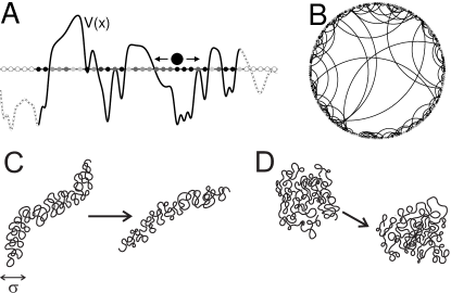
Figure 1: Random hopping along heterogeneous polymers. A: A particle (black disc) moving along the chemical axis $x$ experiences a random potential $V(x)$ associated with the random sequence of different types of monomers. When the chain is in a complex folding state, locations that are distant along the chemical axis $x$ may be close in Euclidean space (C,D). The folding topology is determined by a connectivity matrix depicted in B where circular arcs indicate neighborhood in Euclidean space. C: A folding state with a characteristic mesoscopic scale $\sigma$. D: A freely flexible chain with long range connections on all scales. Arrows indicate conformational change over time.

Consider the scenario depicted in Fig. 1. A particle is attached to a hetero-polymer and performs a random walk along the chain. Let $x$ denote the chemical coordinate with an inter-monomer spacing of $a$. The chain is flexible, and rapidly changing its conformational state defined by the Euclidean coordinate $\mathbf{R}(x)$ of each monomer. The heterogeneity of the chain is modeled by a potential $V(x)$ which specifies the probability of the particle being attached to site $x$. In a thermally equilibrated system this probability is proportional to the Boltzmann factor $\exp\left[-\beta V(x)\right]$. The dynamics of the particle is governed by the rate $w(x|y,t)$ of making a transition $y\rightarrow x$ at time $t$. We assume that transitions occur only between monomer sites which are close in Euclidean space, i.e. when $|\mathbf{R}(y,t)-\mathbf{R}(x,t)|\lesssim a$. We make the simplest possible ansatz for this rate to take into account the requirements of Gibbs-Boltzmann statistics, the potential heterogeneity of the chain and the complexity of conformational states,

$$w(x|y,t)=\frac{1}{\tau}\,e^{-\beta[V(x)-V(y)]/2}\Gamma(x,y;t).$$ (1)

where the parameter $\tau$ is the typical microscopic time constant and the function $\Gamma(x,y;t)$ is defined by

$$\Gamma(x,y;t)=\begin{cases}1&\quad\text{if}\quad\left|\mathbf{R}(x,t)-\mathbf{R}(y,t)\right|\leqslant a,\\ 0&\quad\text{otherwise}.\end{cases}$$ (2)

$\Gamma(x,y;t)$ reflects the dependence of transitions on the time dependent conformational state of the chain and is symmetric, i.e. $\Gamma(x,y;t)=\Gamma(y,x;t)$. The function $\Gamma(x,y;t)$ can be interpreted as a time dependent connectivity matrix (Fig. 1B). The propagator $p(x,t)$ of a particle initially ($t=0$) at the origin evolves according to the master equation,

$$\partial_{t}\,p(x,t)=\int\textrm{d}y\,\left[w(x|y,t)\,p(y,t)-w(y|x,t)\,p(x,t)\right]$$ (3)

in which the rate is given by Eq. (1). The geometrical factor $\Gamma(x,y;t)$ varies erratically and can be regarded as a stochastic process evolving on a time scale $\tau_{g}$, which is generally different from the hopping time constant $\tau$. Averaging (denoted by $\left[\cdot\right]$) over conformational states the dynamics reads $\partial_{t}\,\left[p\right]=\left[\mathcal{L}\,p\right]$ where the operator $\mathcal{L}$ is defined by the rhs of Eq. (3). If conformational changes occur on smaller time scales than the hopping ($\tau_{g}\ll\tau$) we may substitute$\left[\mathcal{L}\,p\right]\approx\left[\mathcal{L}\right]\left[p\right]$, which represents a mean field approximation. In mean field, Eq. (1) is given by

$$\left[w(x|y,t)\right]=\frac{1}{\tau}e^{-\beta\left[V(x)-V(y)\right]/2}\rho(|x-y|),$$ (4)

where $\rho(|x-y|)=\left[|\mathbf{R}(x,t)-\mathbf{R}(y,t)|\leq a\right]$ is the probability that two given sites $x$ and $y$ are neighbors in Euclidean space. If the folding process is stationary, this probability is time independent, and due to translation invariance along the chain it is a decreasing function of distance in chemical space. The specific functional form of $\rho(x)$ determines the asymptotics of Eq. (3). Consider the situation depicted in Fig. 1C., where the chain is knotted such that non-local transitions occur on a typical scale $\sigma>a$. On larger scales $\rho(x)$ vanishes. In this case, a Kramers-Moyal expansion of the rhs of Eq. (3) yields the FPE $\partial_{t}\,p=\nabla V^{\prime}p+D\Delta p$, in which the diffusion coefficient is given by $D\sim(\sigma/a)^{2}/\tau$ and the gradient force is determined by the potential $V(x)$ along the chain. The situation changes drastically for the type of chain sketched in Fig. 1D. For a freely flexible chain the quantity $\rho(x)$ follows an inverse power law with increasing chemical distance, i.e. $\rho(x)\sim 1/|x|^{1+\mu}$. Typically $\mu<2$ de Gennes (1979) and thus $\rho(x)$ lacks a well defined variance and consequently a typical scale in long range transitions. A particle moving along such a chain will behave superdiffusively and perform a Lévy flight in chemical coordinates. Inserting $\rho(x)\sim 1/|x|^{1+\mu}$ with $0<\mu<2$ into Eq. (4) and subsequently into Eq. (3) the asymptotics is governed by a fractional Fokker-Planck equation (FFPE),

$$D^{-1}\partial_{t}\,p=e^{-\beta V/2}\,\Delta^{\mu/2}\,e^{\beta V/2}\,p-p\,e^{\beta V/2}\,\Delta^{\mu/2}\,e^{-\beta V/2}.$$ (5)

A detailed derivation is given in Ref. Brockmann and Sokolov (2002). Here, $D$ is the generalized diffusion coefficient and the operator $\Delta^{\mu/2}$ is a generalization of the ordinary Laplacian,

$$\left(\Delta^{\mu/2}f\right)(x)=C_{\mu}\int\textrm{d}y\,\frac{f(y)-f(x)}{|x-y|^{1+\mu}}$$ (6)

with $C_{\mu}=\pi^{-1}\Gamma(1+\mu)\sin(\pi\mu/2)$. In contrast to the ordinary Laplacian, $\Delta^{\mu/2}$ is a non-local, singular integral operator, reflecting the superdiffusive behavior of the process. The boundary case $\mu=2$ represents the limit of ordinary diffusion, i.e. Eq. (5) reduces to an ordinary FPE. When the potential vanishes, $V\equiv 0$, Eq. (5) becomes $\partial_{t}\,p=D\Delta^{\mu/2}p$ and is solved by the propagator of the symmetric Lévy stable process of index $\mu$, i.e. $p(x,t)=(Dt)^{1/\mu}\,L_{\mu}\left(x/(Dt)^{1/\mu}\right)$ with $L_{\mu}(z)=(2\pi)^{-1}\int\textrm{d}k\,\exp(ikz-|k|^{\mu})$ Brockmann and Sokolov (2002). In its general form Eq. (5) describes the dynamics of Lévy flights in external potentials obeying Gibbs-Boltzmann thermodynamics.

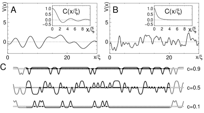
Figure 2: A: A random phase potential with a power spectrum $S(k)=2\xi\,\Theta(|k-\pi/2\xi|)$ where $\Theta$ is the Heaviside function. The correlation function $C(x)=2/\pi\sin(\pi x/2\xi)/(x/\xi)^{2}$ decays in an oscillatory fashion (inset). The potential $V(x)$ varies smoothly around zero. B: A potential with exponential power spectrum $S(k)=2\xi\exp\left[-2\xi|k|/\pi\right]$ and Lorentzian correlation function $C(x)=\left[1+(\pi x/2\xi)^{2}\right]^{-1}$. The potential $V(x)$ shows more structure on a finer scale. C: Copolymers with different relative concentrations $c$ of monomer types (gray and black).

In the following we investigate the relaxation properties of Eq. (5) in random potentials $V$. Since the shape of the potential is determined by the ordering of different types of monomers along the chain, $V(x)$ will be bounded and fluctuate about some average. Furthermore, it will generally possess a typical correlation length $\xi$. Without loss of generality we let $\left\langle V\right\rangle=0$ and $\left\langle V^{2}\right\rangle=V_{0}^{2}$. The correlation length $\xi$ is defined by $\xi=V_{0}^{-2}\int_{0}^{\infty}\textrm{d}y\,C(y)$ where $C(y)=\left\langle V(y)V(0)\right\rangle$ is the correlation function. The most straightforward way to incorporate these attributes into a model is by using Gaussian random phase potentials,

$$V(x)=\frac{1}{2\pi}\int\textrm{d}k\,\phi(k)\,e^{-i(kx+\vartheta(k))},$$ (7)

which are defined by a set of random uncorrelated phases $\vartheta(k)$ (with $\vartheta(k)=-\vartheta(-k)$) and the power spectrum $S(k)=\int\textrm{d}x\,e^{ikx}C(x)$ (with $\phi(k)\phi^{\star}(k^{\prime})=2\pi S(k)\delta(k-k^{\prime})$). The pdf associated with this choice of $V(x)$ is Gaussian with zero mean and variance $V_{0}^{2}=(2\pi)^{-1}\int\textrm{d}k\,S(k)$. Fig. 2A. and 2B. show two realizations of random phase potentials, each one with a different power-spectrum (and correlation function).

The relaxation properties are determined by the eigenvalue spectrum $E(k)$ of the evolution operator $\mathcal{L}$ defined by the rhs of Eq. (5). In order to compute the spectrum, the FFPE can be transformed by means of $p(x,t)=e^{-\beta V(x)/2}\psi(x,t)$. This yields a fractional Schrödinger equation with identical spectral properties,

$$\partial_{t}\,\psi = -\mathcal{H}\psi\qquad\textrm{with}$$ (8)

$$\mathcal{H} = D\left(-\Delta^{\mu/2}+U\right).$$ (9)

The operator $\mathcal{H}$ is symmetric and the effective potential $U$ is related to the original potential $V$ by $U(x)=e^{\epsilon v}\Delta^{\mu/2}e^{-\epsilon v}$, where $v(x)=V/V_{0}$ is a rescaled potential of unit variance and $\epsilon=\beta V_{0}/2=V_{0}/2k_{B}T$ is the potential strength in units of $k_{B}T$.

For vanishing potential $\epsilon=0$, we have $U\equiv 0$ and $\mathcal{H}_{0}=D\Delta^{\mu/2}$ which describes free superdiffusion when $\mu<2$. The spectrum of $\mathcal{H}_{0}$ is given by $E_{0}(k)=Dk^{\mu}$. The wave number $k>0$ defines the spatial scale of the corresponding mode. When a potential is present, the spectrum can be written as $E(k)=D_{\mu}(k;\epsilon)\,k^{\mu}$ where $D_{\mu}(k;\epsilon)$ quantifies the relaxation properties on scales $\simeq k^{-1}$ with the unperturbed $k^{\mu}$-behavior as a reference. If $D_{\mu}(k;\epsilon)/D<1$ the process relaxes more slowly compared to free superdiffusion. The spectrum $E(k)$ can be obtained for weak potentials by perturbation theory. If $\epsilon\ll 1$, the effective potential $U$ can be treated as a small perturbation, for $U=\mathcal{O}(\epsilon)$. Up to second order in $\epsilon$ the quantity $D_{\mu}(k;\epsilon)$ reads

$$D_{\mu}(k;\epsilon)/D=\left(1-4\epsilon^{2}G_{\mu}(k)\right),$$ (10)

where the effect on relaxation is provided by the function

$$G_{\mu}(k) =\frac{1}{8\pi}\int\textrm{d}q\,S(q)\,g_{\mu}(k/q)\quad\textrm{with}$$ (11)

$$g_{\mu}(z) =\frac{1}{z^{\mu}}\left(\frac{1}{(1+z)^{\mu}-z^{\mu}}+\frac{1}{|1-z|^{\mu}-z^{\mu}}-2\right).$$ (12)

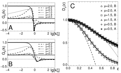
Figure 3: Ralaxation for various Lévy exponents $\mu$(inset) and random phase potentials. Panel A (B) corresponds to the potential in figure 2A(B). $\lg[k\xi]$ denotes the decadic logarithm. The gray lines indicate the limits $G_{\mu}(k\rightarrow 0)$ for $\mu=2$ (upper line) and $\mu<2$ (lower line), see Eq. (13). Panel C depicts the generalized diffusion coefficient $D_{\mu}(\epsilon)$ for the potential in figure 2A(B) and for three Lévy exponents $\mu$. The dashed and dotted lines are the results obtained from perturbation theory, i.e. $D_{\mu}(\epsilon)=1-4\epsilon^{2}$ ($\mu=2$) and $D_{\mu}(\epsilon)=1-\epsilon^{2}$ ($\mu<2$).

Figs. 3A and 3B depict $G_{\mu}(k)$ as a function of $k$ in units of the inverse correlation length $\xi^{-1}$ for the two types of random phase potentials defined in Fig. 2A and 2B. The solid line depicts the limiting case of ordinary diffusion ($\mu=2$). The potential slows down the ordinary diffusion process ($G_{\mu}(k)>0$) on scales larger than the correlation length, and speeds it up ($G_{\mu}(k)<0$) on scales smaller than $\xi$. The function $G_{\mu}(k)$ has a pronounced minimum at $k\approx\xi^{-1}$. Moderately superdiffusive processes ($\mu\gtrsim 1$) behave in a similar fashion, exhibiting the highest variation for $k\approx\xi^{-1}$. On the other hand, $G_{\mu}(k)$ differs strongly for different $\mu$ in the asymptotic regime $k\ll\xi^{-1}$. Note also that on small scales ($k>\xi^{-1}$) almost all processes relax faster than without the potential. In fact, $G_{\mu}(k)<0$ for $2\geq\mu\geq\mu_{c}$ where $\mu_{c}=2-\ln 3/\ln 2\approx 0.415$. Surprisingly, this is no longer valid for strongly superdiffusive processes with $\mu<\mu_{c}$. For instance, in the case $\mu=0.2$ (dashed line in Figs. 3A and 3B) $G_{\mu}(k)$ is positive for $k>\xi^{-1}$, implying that strongly superdiffusive processes are slowed down even on small scales. Comparing potential types, we see that the relaxation is different for each potential, but these differences become less important in the asymptotic regime, which is governed by $G_{\mu}(k)$ as $k\rightarrow 0$. This limit can be computed from Eqs. (11, 12), observing that $\int_{0}^{\infty}\textrm{d}q\,S(q)=\pi$ and $g_{2}(z\rightarrow 0)=1$ and $g_{\mu<2}(z\rightarrow 0)=1/4$,

$$\lim_{k\rightarrow 0}G_{\mu}(k)=\begin{cases}1/4&\quad\mu<2\\ 1&\quad\mu=2,\end{cases}$$ (13)

Hence, the asymptotic behavior is universal, with the exception of the limiting case of ordinary diffusion, and is independent of properties of the potential. The range of validity of the limit (13), however, strongly depends on $\mu$. The limit is not attained for marginal exponents (e.g. $\mu=0.2$ and $1.9$) even on scales several orders of magnitude larger than the correlation length (Fig. 3A and 3B). The above results are valid for small potential strengths $\epsilon$. For higher effective potential strengths we investigate the asymptotics numerically. The quantity of interest is the normalized generalized diffusion coefficient $D_{\mu}(\epsilon)$ defined by

$$D_{\mu}(\epsilon)=\lim_{k\rightarrow 0}D_{\mu}(k;\epsilon)/D.$$ (14)

In the perturbative regime Eqs. (10) and (14) yield the universal relation $D_{\mu}(\epsilon)=1-\epsilon^{2}$ for $\mu<2$ and $D_{\mu}(\epsilon)=1-4\epsilon^{2}$ for ordinary diffusion. Figs. 3C and 3D compare these results to those obtained numerically. Although the numerics deviates from perturbation theoretic predictions for greater potential strengths $\epsilon$, the universality still holds, i.e. the asymptotics ($k\rightarrow 0$) is independent of $\mu$ and of the statistical properties of the potential. The crucial property is the non-locality of the process (i.e. $\mu=2$ vs. $\mu\neq 2$). Thus, as soon as the folding properties of the chain permit scale free transitions ($\mu\neq 2$), the behavior of $D_{\mu}(\epsilon)$ changes abruptly.

Figure 4: The generalized diffusion coefficient $D_{\mu}(\epsilon)$ for the copolymer potential, i.e. Eq. (15) at three relative monomer concentrations. The potentials (Fig. 2C) either possess sparsely distributed peaks ($c=0.05$), troughs ($c=0.95$) or vary uniformly ($c=0.5$). Dashed ($\mu=2$) and dotted ($\mu=1$) lines represent perturbation theoretic results. A: $D_{\mu}(\epsilon)$ for a Lévy flight ($\mu=1$) is different for each potential. B: $D_{\mu}(\epsilon)$ for ordinary diffusion ($\mu=2$) is independent of $c$, the curves coincide.

The pdf of random phase potentials is symmetric with respect to the mean, i.e. a value $V$ is as likely to occur as $-V$ along the chain. For a number of hetero-polymers this assumption is inadequate. Consider the simple model copolymer depicted in Fig. 2C. The chain consists of a random arrangement of monomers, each one equipped with an intrinsic local potential parity $v_{-}$ and $v_{+}$, with $-v_{-}=v_{+}>0$ and an interaction range which we assume to be a Gaussian $f(x-x_{n})$ centered at the monomer site $x_{n}$,

$$V(x)=\sum v_{n}\,f(x-x_{n}),$$ (15)

with $f(x)=\exp[-x^{2}/2\sigma^{2}]$ and $\sigma\approx a$. The $v_{n}$ are randomly drawn from a pdf $p(v)=c\delta(v-v_{-})+(1-c)\delta(v-v_{+})$. The relative concentration of low and high energy monomers is given by $c$ and $1-c$, respectively. The parameter $c$ determines the shape of the overall potential. When $c<1/2$ ($c>1/2$) the potential consists of a series of localized peaks (troughs). Mean and variance of the potential are $\left\langle V\right\rangle=(1-c)\,v_{-}+c\,v_{+}$ and $\left\langle(V-\left\langle V\right\rangle)^{2}\right\rangle=(1-c)\,c\,\delta v^{2}$ with $\delta v=v_{+}-v_{-}$. Figs. 4A and 4B depict the results obtained for the generalized diffusion coefficient $D_{\mu}(\epsilon)$ on these types of copolymers for three values of $c$, each one representing one of the situations depicted in Fig. 2C. The parameter $\delta v$ was chosen such that the variance is identical in all potentials. Although the value of $D_{\mu}(\epsilon)$ in the weak potential regime ($\epsilon\ll 1$) is consistent with the one observed in random phase potentials, for greater values of $\epsilon$ a striking deviation occurs. On one hand, the ordinary diffusion process ($\mu=2$) is nearly insensitive to the shape of the potential, all functions $D_{2}(\epsilon)$ coincide. On the other hand, the superdiffusive process exhibits a more (less) pronounced decrease with increasing $\epsilon$ when $c=0.95$ ($c=0.05$) as compared to an unbiased concentration of monomer types.

The results reported in this Letter predict for superdiffusive behavior on folding polymers that the dispersion speed depends strongly on the specific arrangement of various types of monomers. This is in sharp contrast to the case of ordinary diffusion, which solely depends on magnitude variations of the potential. Therefore we expect that potential heterogeneity is an essential ingredient in superdiffusive translocation phenomena of proteins along biopolymers.