Multi-Overlap Simulations for Transitions between Reference Configurations

Abstract

We introduce a new procedure to construct weight factors, which flatten the probability density of the overlap with respect to some pre-defined reference configuration. This allows one to overcome free energy barriers in the overlap variable. Subsequently, we generalize the approach to deal with the overlaps with respect to two reference configurations so that transitions between them are induced. We illustrate our approach by simulations of the brainpeptide Met-enkephalin with the ECEPP/2 energy function using the global-energy-minimum and the second lowest-energy states as reference configurations. The free energy is obtained as functions of the dihedral and the root-mean-square distances from these two configurations. The latter allows one to identify the transition state and to estimate its associated free energy barrier.

I Introduction

Markov chain Monte Carlo (MC) simulations, for instance by means of the Metropolis method [1], are well suited to simulate generalized ensembles. Generalized ensembles do not occur in nature, but are of relevance for computer simulations (see [2, 3, 4] for recent reviews). They may be designed to overcome free energy barriers, which are encountered in Metropolis simulations of the Gibbs-Boltzmann canonical ensemble. Generalized ensembles do still allow for rigorous estimates of the canonical expectation values, because the ratios between their weight factors and the canonical Gibbs-Boltzmann weights are exactly known.

Umbrella sampling [5] was one of the earliest generalized-ensemble algorithms. In the multicanonical approach [6, 7] one weights with a microcanonical temperature, which corresponds, in a selected energy range, to a working estimate of the inverse density of states. Expectation values of the canonical ensembles can be constructed for a wide temperature range, hence the name “multicanonical”. Here, “working estimate” means that running the updating procedure with the (fixed) multicanonical weight factors covers the desired energy range. The Markov process exhibits random walk behavior and moves in cycles from the maximum (or above) to the minimum (or below) of the chosen energy range, and back. A working estimate of the multicanonical weights allows for calculations of the spectral density and all related thermodynamical observables with any desired accuracy by simply increasing the MC statistics. Thus, we have a two-step approach: The first step is to obtain the working estimate of the weights, and the second step is to perform a long production run with these weights. There is no need for that estimate to converge towards the exact inverse spectral density. Once the working estimate of the weights exists, MC simulations with frozen weights converge and allow one to calculate thermodynamical observables with, in principle, arbitrary precision. Various methods, ranging from finite-size scaling estimates [8] in case of suitable systems to general purpose recursions [9, 10, 11], are at our disposal to obtain a working estimate of the weights.

In the present article we deal with a variant of the multicanonical approach: Instead of flattening the energy distribution, we construct weights to flatten the probability density of the overlap with a given reference configuration. This allows one to overcome energy barriers in the overlap variable and to get accurate estimates of thermodynamic observables at overlap values which are rare in the canonical ensemble. A similar concept was previously used in spin glass simulations [12], but there is a crucial difference: In Ref.[12] the weighting was done for the self-overlap of two replicas of the system and a proper name would be multi-self-overlap simulations, while in the present article we are dealing with the overlap to a predefined configuration.

We next generalize our approach to deal with two reference configurations so that transitions between them become covered and our method allows one then to estimate the transition states and its associated free energy barrier. We have in mind situations where experimentalists determined the reference configurations and observed transitions between them, but an understanding of the free energy landscape between the configurations is missing. An example would be the conversion from a configuration with $\alpha$ helix structures to a native structure which is mostly in the $\beta$ sheet, as it is the case for $\beta$-lactoglobulin [13, 14].

The paper is organized as follows: In the next section we describe the algorithmic details, using first one and then two reference configurations. In particular, a two-step updating procedure is defined, which is typically more efficient than the conventional one-step updating. Moreover, based on the sums of uniformly distributed random numbers, a method to obtain a working estimate of the multi-overlap weights is introduced. In section III we illustrate the method for a simulation with the pentapeptide Met-enkephalin. Our simulations use the all-atom energy function ECEPP/2 (Empirical Conformational Energy Program for Peptides [15]) and rely on its implementation in the computer package SMMP (Simple Molecular Mechanics for Proteins [16]). We use as reference configurations the global energy minimum (GEM) state, which has been determined by many authors [17, 18, 19, 20, 21], and the second lowest-energy state, as identified in Refs.[19, 22]. While our overlap definition relies on a distance definition in the space of the dihedral angles, it turns out that for the data analysis the use of the root-mean-square (rms) distance is crucial. It is only in the latter variable that one obtains a clear picture of the transition saddle point in the two-dimensional free energy diagram. In the final section a summary of the present results and an outlook with respect to future applications are given.

II Multi-Overlap Metropolis Algorithm

In this section we explain the details of our multi-overlap algorithm. The overlap of a configuration versus a reference configuration is defined in the next subsection. In the second subsection we discuss details of the updating. To achieve step one of the method, i.e., the construction of a working estimate of the multi-overlap weights, one could employ a similar recursion as the one used in [12] or explore the approach of [11]. Instead of doing so, we decided to test a new method: At infinite temperature, $\beta=0$, the overlap distributions can be calculated analytically (see subsection II D). We use this as starting point and estimate the overlap weights at the desired temperature by increasing $\beta$ in sufficiently small steps so that the entire overlap range remains covered. In the final subsection we define the overlap with respect to two distinct reference configurations to cover the transition region between them.

A Definition of the overlap

There is a considerable amount of freedom in defining the overlap of two configurations. For instance, one may rely on the rms distance between configurations, and in subsection III D we analyze some of our results in this variable. However, the computation of the rms distance is slow and for MC calculations it is important to rely on a computationally fast definition. Therefore, we define the overlap in the space of dihedral angles by, as it was already used in [24],

$$q\ =\ (n-d)/n\ ,$$ (1)

where $n$ is the number of dihedral angles and $d$ is the distance between configurations defined by

$$d\ =\ ||v-v^{1}||\ =\ {1\over\pi}\sum_{i=1}^{n}d_{a}(v_{i},v_{i}^{1})\ .$$ (2)

Here, $v_{i}$ is our generic notation for the dihedral angle $i$, $-\pi<v_{i}\leq\pi$, and $v^{1}$ is the vector of dihedral angles of the reference configuration. The distance $d_{a}(v_{i},v_{i}^{\prime})$ between two angles is defined by

$$d_{a}(v_{i},v_{i}^{\prime})\ =\ \min(|v_{i}-v_{i}^{\prime}|,2\pi-|v_{i}-v_{i}^{\prime}|)\ .$$ (3)

The symbol $||.||$ defines a norm in a vector space. In particular, the triangle inequality holds

$$||v^{1}-v^{2}||\leq||v^{1}-v||+||v-v^{2}||\ .$$ (4)

For a single angle we have

$$0\leq|v_{i}-v_{i}^{1}|\leq\pi\ \Rightarrow\ 0\leq d\leq n\ .$$ (5)

At $\beta=0$ (i.e., infinite temperature)

$$d_{i}\ =\ {1\over\pi}\,d_{a}(v_{i},v_{i}^{1})$$ (6)

is a uniformly distributed random variable in the range $0\leq d_{i}\leq 1$ and the distance $d$ in (2) becomes the sum of $n$ such uniformly distributed random variables, which allows for an exact calculation of its distribution.

B Multi-overlap weights

We choose a reference configuration of $n$ dihedral angles $v_{i}^{1},\,(i=1,\dots,n)$ to define the dihedral distance (2). We want to simulate the system with weight factors that lead to a random walk (RW) process in the dihedral distance $d$,

$$d<d_{\min}\ \to\ d>d_{\max}~{}~{}{\rm and~{}~{}back}\ .$$ (7)

Here, $d_{\min}$ is chosen sufficiently small so that one can claim that the reference configuration has been reached, e.g., a few percent of $n/2$, which is the average $d$ at $T=\infty$. The value of $d_{\max}$ has to be sufficiently large to introduce a considerable amount of disorder, e.g., $d_{\max}=n/2$. In the following we call one event of the form (7) a random walk cycle (RWC).

One possibility is to choose weight factors which give a flat probability density in the dihedral distance range $0\leq d\leq n/2$, falling off for $d>n/2$ by keeping the $d$-dependence of the weight constant for $d\geq n/2$. This is quite similar to multimagnetical simulations [8], for which the external magnetic field takes the place of the reference configuration. The analogy becomes obvious, when the external field is defined via a ghost spin, which couples to all other spins. For instance, the spins $\vec{s}$ of the Heisenberg ferromagnet are three-dimensional vectors of magnitude $\vec{s}^{\,2}=1$. Their interaction with an external magnetic field $\vec{H}$ can be written as

$$\vec{H}\cdot\sum_{i}\vec{s}_{i}=H\sum_{i}\vec{s}_{H}\cdot\vec{s}_{i}=N\,H\,q\ ,$$ (8)

where $\vec{s}_{H}$ is the unit vector in the direction of the magnetic field, $\vec{s}_{i}$ is the Heisenberg spin at site $i$, $N$ is the number of spins, and $q$ is the overlap of the spin configuration with the reference configuration $\vec{s}_{H}$:

$$q={1\over N}\sum_{i}\vec{s}_{H}\cdot\vec{s}_{i}\ .$$ (9)

Using the multi-overlap language [12], the multi-magnetical [8] weight factors may then be re-written as

$$\exp\left(-\beta E+S(q)\right)=w_{c}(E)\,w_{q}(q)~{},$$ (10)

where

$$w_{c}(E)=\exp(-\beta\,E)~{},$$ (11)

and $E=-\sum_{\langle ij\rangle}\vec{s}_{i}\cdot\vec{s}_{j}$ is energy function of the Heisenberg ferromagnet (the sum is over nearest neighbor spins). Here, $S(q)$ has the meaning of a microcanonical entropy of the overlap parameter, which has to be determined so that the probability density becomes flat in $q$. Weights for other than the flat distribution have also been discussed in the literature, e.g., Ref.[25], on which we shall comment in connection with figure 7 below.

C The updating procedure

In essence, there are two ways to implement the update.

1. Combine the multi-overlap and the canonical weights to one probability, which is accepted or rejected in one random step.

2. Accept or reject the multi-overlap and the canonical probabilities sequentially in two random steps.

1 One-step updating

As defined in equations (10) and (11), the weight factor is a product of $w_{c}(E)$ and $w_{q}(d)$, where $w_{c}(E)$ is the usual, canonical Gibbs-Boltzmann factor and $w_{q}(d)$ is the multi-overlap weight factor, where we now use the distance $d$ from the reference configuration (instead of the overlap $q$) as argument. As is clear from equation (1), the use of either $q$ or $d$ as argument is equivalent, while in the presentation of results the use of either variable can have intuitive advantages. In the one-step updating we combine the weights to

$$w(E,d)\ =\ w_{c}(E)\,w_{q}(d)~{},$$ (12)

and accept or reject newly proposed configurations in the standard Metropolis way. Notably, the calculation of $w_{q}(d)$ (a simple table lookup) is very fast compared with the calculation of $w_{c}(E)$. Therefore, the following two-step procedure is of interest.

2 Two-step updating

Suppose that the present configuration is $(d,E)$ and a new configuration $(d^{\prime},E^{\prime})$ is proposed:

$$(d,E)\ \to\ (d^{\prime},E^{\prime})\ .$$ (13)

We can sequentially first accept or reject with the $w_{q}(d)$ probabilities and then conditionally, when the $d$-part is accepted, with the $w_{c}(E)$ probabilities.

Proof: We show detailed balance for two subsequent updates of the same dihedral angle with the two-step procedure. There are four cases with probabilities of acceptance:

$$P_{i},\ i=1,2,3,4\,.$$ (14)

They are listed in the following:

$$1.~{}~{} w_{q}(d^{\prime})\geq w_{q}(d)~{}~{}{\rm and}~{}~{}w_{c}(E^{\prime})\geq w_{c}(E):$$ (16)

$$P_{1}=1,$$

$$2.~{}~{} w_{q}(d^{\prime})\geq w_{q}(d)~{}~{}{\rm and}~{}~{}w_{c}(E^{\prime})<w_{c}(E):$$ (18)

$$P_{2}=w_{c}(E^{\prime})/w_{c}(E),$$

$$3.~{}~{} w_{q}(d^{\prime})<w_{q}(d)~{}~{}{\rm and}~{}~{}w_{c}(E^{\prime})\geq w_{c}(E):$$ (20)

$$P_{3}=w_{q}(d^{\prime})/w_{q}(d),$$

$$4.~{}~{} w_{q}(d^{\prime})<w_{q}(d)~{}~{}{\rm and}~{}~{}w_{c}(E^{\prime})<w_{c}(E):$$ (22)

$$P_{4}=w_{q}(d^{\prime})\,w_{c}(E^{\prime})/[w_{q}(d)\,w_{c}(E)].$$

For the inverse move

$$(d^{\prime},E^{\prime})\ \to\ (d,E)$$ (23)

with probabilities of acceptance

$$P^{\prime}_{i},\ i=1,2,3,4,$$ (24)

the cases are:

$$1.~{}~{} w_{q}(d)\leq w_{q}(d^{\prime})~{}~{}{\rm and}~{}~{}w_{c}(E)\leq w_{c}(E^{\prime}):$$ (26)

$$P^{\prime}_{1}=w_{q}(d)\,w_{c}(E)/[w_{q}(d^{\prime})\,w_{c}(E^{\prime})],$$

$$2.~{}~{} w_{q}(d)\leq w_{q}(d^{\prime})~{}~{}{\rm and}~{}~{}w_{c}(E)>w_{c}(E^{\prime}):$$ (28)

$$P^{\prime}_{2}=w_{q}(d)/w_{q}(d^{\prime}),$$

$$3.~{}~{} w_{q}(d)>w_{q}(d^{\prime})~{}~{}{\rm and}~{}~{}w_{c}(E)\leq w_{c}(E^{\prime}):$$ (30)

$$P^{\prime}_{3}=w_{c}(E)/w_{c}(E^{\prime}),$$

$$4.~{}~{} w_{q}(d)>w_{q}(d^{\prime})~{}~{}{\rm and}~{}~{}w_{c}(E)>w_{c}(E^{\prime}):$$ (32)

$$P^{\prime}_{4}=1.$$

For the ratios we find

$${P_{i}\over P^{\prime}_{i}}\ =\ {w_{q}(d^{\prime})\,w_{c}(E^{\prime})\over w_{q}(d)\,w_{c}(E)}~{},$$ (33)

independently of $i=1,2,3,4$. Therefore, we have constructed a valid Metropolis updating procedure.

D Sums of a uniformly distributed random variable

To calculate the overlap weights at infinite temperature, we consider the sum

$$u^{r}\ =\ x^{r}_{1}+\dots+x^{r}_{n}$$ (34)

of the random variables $x^{r}_{j}$ ($j=1,\cdots,n$), each uniformly distributed in the interval $[0,1)$ and derive a recursion formula for the probability density $f_{n}(u)$ of this distribution. Care is taken to cast the recursion in a form which allows for a numerically stable implementation [26] over a reasonably large range of $n$.

Let us recall the probability density of the uniform distribution:

$$f_{1}(x)\ =\ \cases{1,~{}{\rm for}~{}0\leq x<1,\cr 0,~{}{\rm otherwise}.}$$ (35)

To derive the recursion formula for the probability density of the random variable (34), it is convenient to cast it in the form

$$f_{n}(u)\ =\ \sum_{k=1}^{n}f_{n,k}(x_{k})~{}~{}{\rm with}~{}~{}\ x_{k}=u-k+1,$$ (36)

where

$$f_{n,k}(x)\ =\ \cases{\displaystyle{\sum_{i=0}^{n-1}a_{n,k}^{i}\,x^{i}},~{}{\rm for}~{}0\leq x<1\\ ,\cr~{}0,~{}{\rm otherwise}.}$$ (37)

The master formula for the recursion is obtained from the convolution

$$f_{n}(u)\ =\ \int_{0}^{u}f_{1}(u-v)\ f_{n-1}(v)\ dv\ .$$ (38)

Let now $u=x+k-1$ with $0\leq x<1$, and equations (35), (36), and (37) imply

$$f_{n,k}(x)\ =\ \int_{k-2+x}^{k-1+x}f_{n-1}(v)\ dv$$ (39)

$$=\ \int_{x}^{1}f_{n-1,k-1}(y)\ dy\ +\ \int_{0}^{x}f_{n-1,k}(y)\ dy\ .$$ (40)

Using equation (37) and performing the integrations, we obtain

$$f_{n,k}(x) = \sum_{i=0}^{n-2}a_{n-1,k-1}^{i}\,{1\over i+1}\ -\ \sum_{i=0}^{n-2}a_{n-1,k-1}^{i}\,{x^{i+1}\over i+1}$$ (41)

$$+ \sum_{i=0}^{n-2}a_{n-1,k}^{i}\,{x^{i+1}\over i+1}\ .$$ (42)

Expanding in powers of $x$ and comparing (37) with (42) allows one to calculate the coefficients $a_{n,k}^{i}$ recursively in a numerically robust way:

$$a_{n,k}^{0}=\sum_{j=0}^{n-1}{a_{n-1,k-1}^{j}\over j+1}\,,\ a_{n,k}^{i}=\sum_{j=0}^{n-1}{a_{n-1,k}^{j}-a_{n-1,k-1}^{j}\over j+1}\ .$$ (43)

Once the coefficients $a_{n,k}^{i}$ are available, one can easily evaluate the probability densities $f_{n}(u)$ and the corresponding cumulative distribution functions.

The probability density (36) takes its maximum value for $u=n/2$. Due to the central limit theorem the fall-off behavior is Gaussian as long as $u$ stays sufficiently close to $n/2$. In the tails, for $u\to 0$ or $u\to n$, the fall-off is much faster than Gaussian, namely an exponential of an exponential as follows from extreme value statistics [27].

E Combination of two weights

In the following the weights with superscript $j$, $w_{q}^{j}(d_{j})$, correspond to two distinct reference configurations $v^{j}$, ($j=1,2$), and $d_{j}$ is the distance from the configuration at hand to the configuration $v^{j}$. Let us assume that multi-overlap simulations with respect to the two reference configurations have been carried out and that the weights, $w_{q}^{1}(d_{1})$ and $w_{q}^{2}(d_{2})$, have been determined so that they sample their distance distributions approximately uniformly.

We want to construct combined weights $w_{q}^{12}(d_{1},d_{2})$ which lead to a RW process between the configurations $v^{1}$ and $v^{2}$. Our choice is

$$w_{q}^{12}(d_{1},d_{2})\ =\ \cases{w_{q}^{1}(d_{1}),~{}~{}{\rm for}~{}~{}d_{1}<d_{2}\,,\cr c_{j}\,w_{q}^{2}(d_{2}),~{}~{}{\rm for}~{}~{}d_{1}\geq d_{2}\,.}$$ (44)

The constant $c_{j}$, with $j$ either 1 or 2, is introduced to allow for smooth transitions from $d_{1}<d_{2}$ to $d^{\prime}_{1}\geq d^{\prime}_{2}$ and vice versa. We determine $c_{j}$ from the analysis of either run 1 (or run 2), which are the (one reference configuration) simulations leading to the weights $w_{q}^{1}(d_{1})$ (or $w_{q}^{2}(d_{2})$). The constant $c_{1}$ is found from run 1 by scanning the time series for configuration for which $d_{1}\geq d_{2}$ holds and which have a one-update transition $(d_{1},d_{2})\to(d^{\prime}_{1},d^{\prime}_{2})$ with $d^{\prime}_{1}<d^{\prime}_{2}$. From these configurations $k$ we determine the constant $c_{1}$ so that

$$\sum_{k}w_{q}^{1}[d_{1}(k)]\ =\ c_{1}\sum_{k}w_{q}^{2}[d_{2}(k)]$$ (45)

holds. Similarly, run 2 may be used to get $c_{2}$. It turns out that the normalized weights almost agree in the transition region and, therefore, the patching (44) works. The dependence of the constant on the run used for its determination is small, and it appears not worthwhile to explore more sophisticated methods.

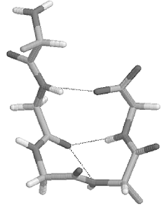
FIG. 1.: Reference configuration 1. Only backbone structure is shown. The N-terminus is on the left-hand side and the C-terminus on the right-hand side. The dotted lines stand for hydrogen bonds. The figure was created with RasMol [23]

It is straightforward to implement the Metropolis updating with respect to the weights (44). For the transition

$$(d_{1},d_{2})\ \to\ (d^{\prime}_{1},d^{\prime}_{2})\,,$$ (46)

one has to distinguish four more cases:

$$1. d_{1}<d_{2}~{}~{}{\rm and}~{}~{}d^{\prime}_{1}<d^{\prime}_{2}\,,$$ (47)

$$2. d_{1}<d_{2}~{}~{}{\rm and}~{}~{}d^{\prime}_{1}\geq d^{\prime}_{2}\,,$$ (48)

$$3. d_{1}\geq d_{2}~{}~{}{\rm and}~{}~{}d^{\prime}_{1}<d^{\prime}_{2}\,,$$ (49)

$$4. d_{1}\geq d_{2}~{}~{}{\rm and}~{}~{}d^{\prime}_{1}\geq d^{\prime}_{2}\,.$$ (50)

Alternatively to the approach outlined, one may combine $d_{1}$ and $d_{2}$ into a new variable $\theta_{d}$ for which the weights are then calculated as in the one-dimensional case. A suitable choice along this line is

$$\theta_{d}={2\over\pi}\,\arctan\left({d_{1}\over d_{2}}\right)\ .$$ (51)

III Met-Enkephalin Simulations

In the following we introduce two reference configurations. Subsequently, we discuss first the results for simulations with one reference configuration and then those involving both reference configurations.

A The reference configurations

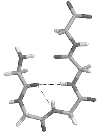
FIG. 2.: Reference configuration 2. See the caption of figure 1 for details.

Met-enkephalin has the amino-acid sequence Tyr-Gly-Gly-Phe-Met. We fix the peptide-bond dihedral angles $\omega$ to $180^{\circ}$, which implies that the total number of variable dihedral angles is $n=19$. We neglect the solvent effects as in previous works. The low-energy configurations of Met-enkephalin in the gas phase have been classified into several groups of similar structures [19, 22]. Two reference configurations, called configuration 1 and configuration 2, are used in the following and depicted in figures 1 and 2, respectively. Configuration 1 has a $\beta$-turn structure with hydrogen bonds between Gly-2 and Met-5, and configuration 2 a $\beta$-turn with a hydrogen bond between Tyr-1 and Phe-4 [22].

For our present work the two reference configurations were obtained by minimizing the GEM and the second lowest energy state of previous literature with respect to the ECEPP/2 energy function. The minimization was performed with the SMMP minimizer [16] and by quenching. Both methods gave identical final energies. In table I we list the variable dihedral angles of the configurations before and after this minimization. The initial dihedral angles for the GEM are taken from table 1 of Ref.[21] and the initial dihedral angles for the second lowest energy state B are from table 1 of Ref.[19]. In table I we give the angles in degrees, while for the MC simulations radians were used as in equations (1) and (2) for the overlap. Our labeling of the residues follows the SMMP convention and deviates from those of Refs.[21, 19].

TABLE I.: Met-enkephalin reference configurations. The columns $\rm GEM_{min}$ and $\rm B_{min}$ correspond to configuration 1 and configuration 2, respectively.

Residue	Angle	GEM [21]	$\rm GEM_{min}$	B [19]	$\rm B_{min}$
1	$\chi_{1}$	$-179.9$	$-179.8$	$-179$	$+179.4$
1	$\chi_{2}$	$-111.3$	$-111.4$	$~{}-95$	$~{}-94.3$
1	$\chi_{6}$	$+145.3$	$+145.3$	$+169$	$-179.9$
1	$\phi$	$~{}-86.4$	$~{}-86.3$	$+111$	$~{}+55.7$
2	$\psi$	$+153.7$	$+153.7$	$+157$	$+157.6$
2	$\phi$	$-161.6$	$-161.5$	$~{}-71$	$~{}-70.7$
3	$\psi$	$~{}+71.2$	$~{}+71.1$	$~{}+78$	$~{}+78.0$
3	$\phi$	$~{}+64.1$	$~{}+64.1$	$~{}159$	$+156.5$
4	$\psi$	$~{}-93.5$	$~{}-93.5$	$~{}-37$	$~{}-35.7$
4	$\chi_{1}$	$+179.8$	$+179.8$	$~{}+59$	$~{}+55.3$
4	$\chi_{2}$	$~{}+80.0$	$~{}+80.0$	$~{}+87$	$~{}+86.8$
4	$\phi$	$~{}-81.7$	$~{}-81.7$	$-154$	$-155.7$
5	$\psi$	$~{}-29.2$	$~{}-29.2$	$+151$	$+151.6$
5	$\chi_{1}$	$~{}-65.1$	$~{}-65.1$	$~{}-68$	$~{}-69.4$
5	$\chi_{2}$	$-179.2$	$-179.2$	$+177$	$-176.3$
5	$\chi_{3}$	$-179.3$	$-179.3$	$-179$	$-179.7$
5	$\chi_{4}$	$~{}-60.0$	$~{}-59.9$	$~{}+60$	$~{}+59.9$
5	$\phi$	$~{}-80.8$	$~{}-80.7$	$-140$	$-140.0$
5	$\psi_{t}$	$+143.9$	$+143.5$	$~{}-29$	$~{}-30.6$

The distance between the two minimized configurations is $d=6.62$ ($q=0.652$) and their energies are given in table II.

TABLE II.: Energies (in kcal/mol) of the Met-enkephalin reference configurations 1 and 2.

	Total	Coulomb	Lennard-Jones	H-Bond	Torsion
1	$-$10.72	$+$21.41	$-$27.10	$-$6.21	$+$1.19
2	$~{}-$8.42	$+$22.59	$-$26.38	$-$4.85	$+$0.23

B Simulations with one reference configuration

Each of our multi-overlap simulations at fixed temperature relies on a statistics of 16,777,216 sweeps for which data are recorded in a time series of 524,288 events, i.e., with a stepsize of 32 sweeps. We started most of our simulations with the GEM configuration, but some random starts were also performed and no noticeable differences were encountered.

Starting with the analytical result (36), valid at $\beta=0$, the weights are calculated by increasing $\beta$ (i.e., decreasing the temperature) between simulations slowly so that the RW of each simulation still covers the desired overlap range when using the weight estimates from the previous temperature. Discretization errors due to histograming can be severe and instead of weights which are piecewise constant within each one histogram interval, we used the interpolation of Ref. [6]:

$$\ln w(d)=(1-\alpha)\ln w(d_{i})+\alpha\ln w(d_{i+1})~{},~{}{\rm for}~{}d_{i}\leq d<d_{i+1}~{},$$ (52)

where

$$\alpha=\frac{d-d_{i}}{d_{i+1}-d_{i}}~{}.$$ (53)

Figure 3 depicts the thus obtained weight function estimates from simulations with reference configuration 1. After five simulations we arrive at the physical temperature $T=300\,$K. The same iteration works with reference configuration 2.

FIG. 3.: Weight estimates from simulations with reference configuration 1. From up to down the weight functions correspond to the following temperatures: $230\,$K, $300\,$K, $400\,$K, $700\,$K, $2,000\,$K, $10,000\,$K, $100,000\,$K and infinity ($\beta=0$).

For the values $d_{\min}=0.025\,n$ and $d_{\max}=0.495\,n$, where $n=19$ is the number of angels in (2), we list in table III the number of RWCs (7) achieved at each temperature. We also list the CPU time ratios for the 1-step versus the 2-step updating procedures, which we discussed in the previous section. Especially at high temperatures, which are needed in our approach, the 2-step updating turns out to be more efficient than the 1-step updating and all of our production runs were done with it.

TABLE III.: Number of random walk cycles in the simulations with our two reference configurations. The last column lists the CPU time ratios for 1-step versus 2-step updating.

$T$	Configuration 1	Configuration 2	1-step/2-step
$100,000\,$K	9,458	9,514	3.0
$10,000\,$K	3,122	3,149	1.8
$2,000\,$K	2,893	2,741	1.6
$700\,$K	2,169	2,227	1.5
$400\,$K	1,342	1,693	1.3
$300\,$K	462	610	1.2
$230\,$K	46	41	1.2

We next rely on the peaked distribution function [26] to visualize some of the data kept in the time series of our simulations. The peaked distribution function of a probability density $f(x)$ is defined by

$$F_{\rm peaked}(x)=\cases{F(x)~{}~{}{\rm for}~{}~{}x\leq 0.5\,,\cr 1-F(x)~{}~{}{\rm for}~{}~{}x>0.5\,,}$$ (54)

where

$$F(x)=\int_{-\infty}^{x}dx^{\prime}\,f(x^{\prime})$$ (55)

is the usual cumulative distribution function (see for instance [28]).

FIG. 4.: Canonical, peaked energy distributions obtained by re-weighting multi-overlap simulations. From left to right the temperatures used are: $230\,$K, $300\,$K, $400\,$K, and $700\,$K.

FIG. 5.: Peaked multi-overlap (left-shifted) and canonical energy distributions at $T=300\,$K and $T=400\,$K.

To visualize how the canonical energy distribution moves when we lower the temperature, we plot in figure 4 the peaked energy distributions as obtained by re-weighting some of the multi-overlap simulations of figure 3 to the canonical ensemble of their simulation temperature. Due to the re-weighting the distributions look precisely as one expects for energies from canonical MC simulations. In contrast to conventional canonical simulations, the raw data feature a considerably larger number of events at low energies. This is illustrated in figure 5, where we plot the $300\,$K and $400\,$K peaked distribution functions of figure 4 together with their raw multi-overlap peaked distributions

FIG. 6.: Probability density of the distance from a multi-overlap simulation at $T=400\,$K (flat) and its canonically re-weighted probability density (peaked).

FIG. 7.: Peaked distribution functions for the forward ($d\to d_{\max}$) and backward ($d\to d_{\min}$) parts of the random walk cycles from a multi-overlap simulation at $T=400\,$K.

FIG. 8.: Left-hand-side ordinate: Specific heat re-weighted from a multicanonical (MUCA) and from a $300\,$K multi-overlap (MUOV) simulation with reference configuration 1. Right-hand-side ordinate: ${dq_{1}\over dT}$ re-weighted from the same simulations, where $q_{1}$ is the overlap with reference configuration 1.

In figure 6 we give an example of the probability density of the distance. For the $400\,$K simulation with reference configuration 1 we plot the probability density of $d_{1}$ as obtained from the multi-overlap simulation together with its canonically re-weighted probability density. The simulation itself is run with the multi-overlap weights from the $700\,$K simulations and the multi-overlap histogram shown is re-weighted to the multi-overlap $400\,$K weights. As expected, we have a flat distribution between 0 and $n/2=9.5$. Moreover, there is a good coverage of configurations close to the GEM, which are highly suppressed in the $400\,$K canonical ensemble. The maximum ratio of the multi-overlap density divided by the canonical density is $6\times 10^{16}$ in this plot.

For the same simulation figure 7 depicts separately the peaked distribution function of the forward and backward RWCs (7). A considerable asymmetry is noticeable and it turns out that the weights of the 1/k ensemble [25] lead to more RWCs than the flat distribution of figure 6. In connection with our simulations this is a lucky circumstance, because the 1/k distribution of weights is in essence the distribution at a somewhat higher temperature than that of the simulation. This increases the flexibility when estimating good weights at a lower temperature from the already existing simulation results at a higher temperature.

For multi-overlap simulations the re-weighting towards low temperatures can work much better than for canonical simulations. This is due to the fact that the low-energy configurations close to low-energy reference configuration are already in the ensemble. This is illustrated in figure 8, where we re-weight the data from a multi-overlap simulation with reference configuration 1 at $T=300\,$K and compare with a conventional multicanonical simulation based on the SMMP package [16]. The specific heat $C_{V}$ and the derivative of the overlap with respect to the temperature are shown. From $200\,$K to $400\,$K the deviations of the results are of the order of the statistical errors, which are not shown for clarity of the figure. Below $200\,$K deviations of the re-weighted overlap simulation from the correct behavior become visible, first in ${dq_{1}\over dT}$ then in $C_{V}$. Such deviations are expected as the low-energy attractor does not lead to a uniform coverage of all low-energy states. The successful re-weighting from high simulation temperatures to lower temperatures is an improvement, because the Metropolis dynamics at high temperatures is faster. But the re-weighting of a multi-overlap simulation to a lower temperature will fail at some point, because the reference configuration introduces a bias towards particular low-energy configurations.

The temperature at which $C_{V}$ and $-{dq_{1}\over dT}$ take peak values correspond to the coil-globule transition temperature $T_{\theta}$ and the folding temperature $T_{f}$ [24]. From figure 8 we read off the following approximate values:

$$T_{\theta}=280\,{\rm K}~{}~{}{\rm and}~{}~{}T_{f}=245\,{\rm K}\ .$$ (56)

C Simulations with two reference configurations

At $300\,$K we combine the weights from the runs with reference configurations 1 and 2 to one weight function according to our equation (44). We record now three different RWCs:

1. With respect to reference configuration 1 from $d_{\min}$ to $d_{\max}$ and back, found 315 times.

2. With respect to reference configuration 2 from $d_{\min}$ to $d_{\max}$ and back, found 545 times.

3. From $d_{\min}$ of reference configuration 1 to $d_{\min}$ of reference configuration 2 and back, found 196 times.

FIG. 9.: Combined weight simulation at $T=300\,$K: Probability densities with respect to the distances $d_{1}$ and $d_{2}$.

In figure 9 we show the probability densities of this simulation with respect to the distances from our reference configurations. They are no longer flat, but a satisfactory coverage in the variables $d_{1}$ and $d_{2}$ is still achieved. Note that both probability densities have peaks at $d=6.62$, which is the distance between configurations 1 and 2. This implies that both reference configurations have been visited with high probability.

D Physics results

We would like to analyze the transitions between our two reference configurations in some detail. For this purpose we use the rms distance, which is defined by

$$d_{\rm rms}=\min\left[\sqrt{{1\over N}\sum_{i=1}^{N}(\vec{x}_{i}-\vec{x}_{i}^{\,j})^{2}}\right]~{},$$ (57)

where $N$ is the number of atoms, $\{\vec{x}^{\,j}_{i}\}$ are the coordinates of the reference configuration $j$, and the minimization is over the translations and rotations of the coordinates of the configuration $\{\vec{x}_{i}\}$.

FIG. 10.: Probability density of the rms distance from the multi-overlap simulation at $T=400\,$K of figure 6, and its canonically re-weighted probability density. The abscissa is the rms distance (Å) in Eq. (57) from the reference configuration 1.

The distance (2) and the rms distance (57) are quite distinct. The reason is that a change of a single dihedral angle in the central parts of the molecule can cause a large deviation in the rms distance. Although the two configurations are then close-by from the point of view of the MC algorithm, physically they are rather far apart, as the similarity of the three-dimensional structures is governed by the rms distance. Therefore, the rms distance distribution deviates considerably from the dihedral distance distribution. We illustrate this by plotting in figure 10 the rms probability density of the 400 K simulation for which the dihedral distance probability density is shown in figure 6.

We now analyze the free-energy landscape [29] from the results of our simulation with combined weights at $300\,$K in some detail. We study the landscape with respect to some reaction coordinates (and hence it should be called the potential of mean force). In order to study the transition states between reference configurations 1 and 2, we first plotted the free-energy landscape with respect to the distances $d_{1}$ and $d_{2}$. However, we did not observe any transition saddle point. A satisfactory analysis of the saddle point becomes possible when the rms distance (instead of the dihedral distance) is used. Figure 11 shows contour lines of the free energy re-weighted to $T=250$ K, which is close to the folding temperature (56). Here, the free energy $F(rms1,rms2)$ is defined by

$$F(rms1,rms2)=-k_{B}T\ln P(rms1,rms2)~{},$$ (58)

where $rms1$ and $rms2$ are the rms distances defined in (57) from the reference configuration 1 and the reference configuration 2, respectively, and $P(rms1,rms2)$ is the (reweighted) probability at $T=250$ K to find the peptide with values $rms1,rms2$. The probability was calculated from the two-dimensional histogram of bin size 0.06 Å$\times$ 0.06 Å. The contour lines were plotted every $2k_{B}T$ ($=0.99$ kcal/mol for $T=250$ K).

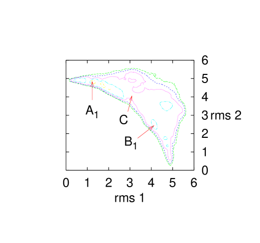
FIG. 11.: Free-energy landscape at $T=250$ K with respect to rms distances (Å) from the two reference configurations, $F(rms1,rms2)$. Contour lines are drawn every $2k_{B}T$. The labels A₁ and B₁ indicate the positions for the local-minimum states at $T=250$ K that originate from the reference configuration 1 and the reference configuration 2, respectively. The label C stands for the saddle point that corresponds to the transition state.

Note that the reference configurations 1 and 2, which are respectively located at $(rms1,rms2)=(0,4.95)$ and $(4.95,0)$, are not local minima in free energy at the finite temperature ($T=250$ K) because of the entropy contributions. The corresponding local-minimum states at A₁ and B₁ still have the characteristics of the reference configurations in that they have backbone hydrogen bonds between Gly-2 and Met-5 and between Tyr-1 and Phe-4, respectively. We remark that we observe in figure 11 another well-defined local minimum state around $(rms1,rms2)=(4.7,3.5)$. This state can also be considered to correspond to configuration 2 because we again observe the backbone hydrogen bond between Tyr-1 and Phe-4. The side-chain structures are, however, more deviated from configuration 2 than B₁, resulting in a larger value of $rms2$.

The transition state C in figure 11 should have intermediate structure between configurations 1 and 2. In figure 12 we show a typical backbone structure of this transition state. We see the backbone hydrogen bond between Gly-2 and Phe-4. This is precisely the expected intermediate structure between configurations 1 and 2, because going from configuration 1 to configuration 2 we can follow the backbone hydrogen-bond rearrangements: The hydrogen bond between Gly-2 and Met-5 of configuration 1 is broken, Gly-2 forms a hydrogen bond with Phe-4 (the transition state), this new hydrogen bond is broken, and finally Phe-4 forms a hydrogen bond with Tyr-1 (configuration 2).

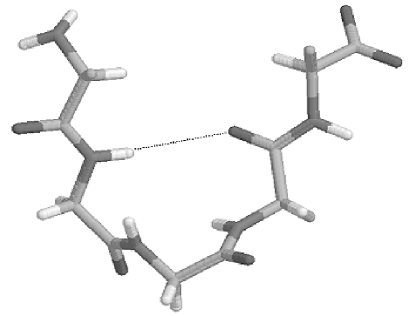
FIG. 12.: The transition state between reference configurations 1 and 2. See the caption of figure 1 for details.

It is interesting to see in figure 11 that there is only one saddle point in the free-energy landscape that connects configurations 1 and 2. Hence, the transition between configurations 1 and 2 always passes through the state C.

In Ref. [22] the low-energy conformations of Met-enkephalin were studied in detail and they were classified into several groups of similar structures based on the pattern of backbone hydorgen bonds. It was found there that below $T=300$ K there are two dominant groups, which correspond to configurations 1 and 2 in the present article. Although much less conspicuous, the third most populated structure is indeed the group that is identified to be the transition state in the present work.

In figures 13 and 14 we show the internal energy landscape and the entropy landscape at $T=250$ K, respectively. Here, the internal energy $U$ is defined by the (reweighted) average ECEPP/2 potential energy:

$$U(rms1,rms2)=<E(rms1,rms2)>~{}.$$ (59)

Here, the average was again calculated from the two-dimensional histogram of bin size 0.06 Å$\times$ 0.06 Å. The entropy $S$ was then calculated by

$$S(rms1,rms2)=\frac{1}{T}\left[U(rms1,rms2)-F(rms1,rms2)\right]~{}.$$ (60)

The landscape in figure 14 is actually $-TS(rms1,rms2)$.

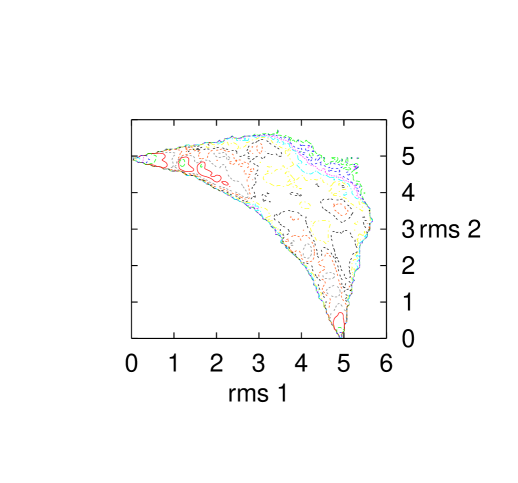
FIG. 13.: Internal energy landscape at $T=250$ K with respect to rms distances (Å) from the two reference configurations, $U(rms1,rms2)$. Contour lines are drawn every $2k_{B}T$.

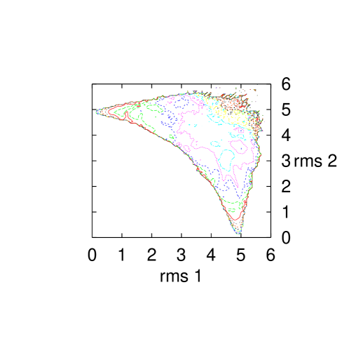
FIG. 14.: Entropy landscape at $T=250$ K with respect to rms distances (Å) from the two reference configurations, $-TS(rms1,rms2)$. Contour lines are drawn every $2k_{B}T$.

Both internal energy and entropy landscapes are more rugged than free energy landscape (we observe much more number of contour lines in figures 13 and  14 than in figure 11). The internal energy has clear local minima at the points $(rms1,rms2)=(0,4.95)$ and $(4.95,0)$, which respectively correspond to configurations 1 and 2, while the entropy landscape has local maxima at these points. These two terms tend to cancel each other, and the free energy landscape is smoothed out.

In table IV we list the numerical values of the free energy, internal energy, and entropy multiplied by temperature at the two local-minimum states (A₁ and B₁ in figure 11) and the transition state (C in figure 11). The internal energy is just the average of the ECEPP/2 potential energy (without any shift of zero point). The free energy was normalized so that the value at A₁ is zero. The values at the coordinates of reference configurations 1 and 2, which are respectively referred to as A₀ and B₀ in the table, are also listed.

TABLE IV.: Free energy, internal energy, entropy multiplied by temperature at $T=250$ K (all in kcal/mol) at the two local-minimum states (A₁ and B₁) and the transition state (C) in figure 11. The values at the coordinates of reference configurations 1 and 2, which are respectively referred to as A₀ and B₀, are also listed. The rms distances are in Å.

Coordinate (rms1,rms2)	$F$	$U$	$-TS$
A1 (1.23, 4.83)	0	$-5.4$	5.4
B1 (4.17, 2.43)	1.0	$-3.5$	4.5
C (3.09, 4.05)	2.2	$-0.8$	3.0
A0 (0.03, 4.95)	15	$-10.5$	26
B0 (4.95, 0.03)	20	$-8.1$	28

Among the five points, A₀ and B₀ are unfavored in free energy mainly due to the large entropy effects, although they are energetically most favored. This means that at this temperature the exact conformations of the reference configurations 1 and 2 are not populated much. The relevant states are rather A₁, B₁, and C. The state A₁ can be considered to be “deformed” configuration 1, and B₁ deformed configuration 2 due to the entropy effects, whereas C is the transition state between A₁ and B₁. Among these three points, the free energy $F$ and the internal energy $U$ are the lowest at A₁, while the entropy contribution $-TS$ is the lowest at C. The free energy difference $\Delta F$, internal energy difference $\Delta U$, and entropy contribution difference $-T\Delta S$ are 1.0 kcal/mol, 1.9 kcal/mol, and $-0.9$ kcal/mol between B₁ and A₁, 2.2 kcal/mol, 4.6 kcal/mol, and $-2.4$ kcal/mol between C and A₁, and 1.2 kcal/mol, 2.7 kcal/mol, and $-1.5$ kcal/mol between C and B₁. Hence, the internal energy contribution and the entropy contribution to free energy are opposite in sign and the magnitude of the former is roughly twice as that of the latter at this temperature.

IV Summary and Conclusions

We have outlined an approach to perform MC simulations which yield the free-energy distribution between two reference configurations. The multi-overlap weights for this purpose were obtained by a novel, iterative process. The main point of this iterative process is not that it is supposed to be more efficient than the recursion that was used in the multi-self-overlap simulations of Ref.[12], but that it is an entirely independent approach, which starts from an analytically controlled limit. Recursions like the one used in [12] are not “foolproof”. For instance, while most of the spin glass replica in Ref.[12] were well-behaved, a few did not complete their recursion after more than an entire year of single processor CPU time. Similar situations could be encountered in all-atom simulations of larger peptides, where the normal multicanonical weight recursion as well as similar multi-overlap weight recursion could fail. The present method provides then an alternative, approaching the physical region from a different limit.

Noticeable, our multi-overlap approach is well-suited to be combined with a recently introduced, biased Metropolis sampling [30]. Namely, the required configurations at higher temperatures are as well necessary for our particular multi-overlap recursion, so that no extra simulations are required in this respect.

On the physical side, we have found that entropy effects are rather important for a small peptide. The effects of entropy on the folding of real proteins in realistic solvent have yet to be studied in detail.

We have also performed the analysis of this paper for Met-enkephalin with variable $\omega$ angles and, in particular, simulated with combined weights at a number of temperatures. The results found are quite similar to those reported in this paper. In future work we intend to analyze the transition between reference configuration for larger systems of actual interest like $\beta$-lactoglobulin.

- [1] N. Metropolis, A.W. Rosenbluth, M.N. Rosenbluth, A.H. Teller, and E. Teller, J. Chem. Phys. 21, 1087 (1953).
- [2] U.H. Hansmann and Y. Okamoto, in Ann. Rev. Comput. Phys. VI, D. Stauffer (ed.) (World Scientific, Singapore, 1999) p. 129.
- [3] A. Mitsutake, Y. Sugita, and Y. Okamoto, Biopolymers (Peptide Science) 60, 96 (2001).
- [4] B.A. Berg, Comp. Phys. Commun. 104, 52 (2002).
- [5] G.M. Torrie and J.P. Valleau, J. Comput. Phys. 23, 187 (1977).
- [6] B.A. Berg and T. Neuhaus, Phys. Lett. B 267, 249 (1991).
- [7] B.A. Berg and T. Celik, Phys. Rev. Lett. 69, 2292 (1992).
- [8] B.A. Berg, U.H. Hansmann, and T. Neuhaus, Phys. Rev. B 47, 497 (1993).
- [9] B.A. Berg, J. Stat. Phys. 82, 323 (1996).
- [10] Y. Sugita and Y. Okamoto, Chem. Phys. Lett. 329, 261 (2000).
- [11] F. Wang and D.P. Landau, Phys. Rev. Lett. 86, 2050 (2001).
- [12] B.A. Berg, A. Billoire, and W. Janke, Phys. Rev. B 61, 12143 (2000).
- [13] K. Kuwajima, H. Yamaya, S. Miwa, S. Sugai, and T. Nagamura, FEBS Lett. 221, 115 (1987).
- [14] D. Hamada, S. Segawa, and S. Goto, Nature Struct. Biol. 3, 868 (1996).
- [15] M.J. Sippl, G. Némethy, and H.A. Scheraga, J. Phys. Chem. 88, 6231 (1984) and references given therein.
- [16] F. Eisenmenger, U.H. Hansmann, S. Hayryan, and C.-K. Hu, Comp. Phys. Commun. 138, 192 (2001).
- [17] Z. Li and H.A. Scheraga, Proc. Natl. Acad. Sci. USA 84, 6611 (1987).
- [18] B. von Freyberg and W.J. Braun, J. Comput. Chem. 12, 1065 (1991).
- [19] Y. Okamoto, T. Kikuchi and H. Kawai, Chem. Lett. 1992, 1275 (1992).
- [20] U.H. Hansmann and Y. Okamoto, J. Comput. Chem. 14, 1333 (1993).
- [21] H. Meirovitch, E. Meirovitch, A.G. Michel, and M. Vásquez, J. Phys. Chem. 98, 6241 (1994).
- [22] A. Mitsutake, U.H. Hansmann, and Y. Okamoto, J. Mol. Graph. and Model. 16, 226 (1998).
- [23] R.A. Sayle and E.J. Milner-White, Trends Biochem. Sci. 20, 374 (1995).
- [24] U.H. Hansmann, M. Masuya and Y. Okamoto, Proc. Natl. Acad. Sci. USA 94, 10652 (1997).
- [25] B. Hesselbo and R. Stinchcombe, Phys. Rev. Let. 74, 2151 (1995).
- [26] B.A. Berg, Markov Chain Monte Carlo Simulations and Their Statistical Analysis I and II, books in preparation.
- [27] E.J. Gumbel, Statistics of Extremes, Columbia University Press, New York, 1958.
- [28] W.H. Press, B.P. Flannery, S.A. Teukolsky and W.T. Vetterling, Numerical Recipes in Fortran, Second Edition, Cambridge University Press, Cambridge, 1992.
- [29] U.H. Hansmann, Y. Okamoto, and J.N. Onuchic, PROTEINS: Structure, Function, and Genetics 34, 472 (1999).
- [30] B.A. Berg, cond-mat/0209413, to be published in Phys. Rev. Lett.