Scale free networks from a Hamiltonian dynamics

Abstract

Contrary to many recent models of growing networks, we present a model with fixed number of nodes and links, where it is introduced a dynamics favoring the formation of links between nodes with degree of connectivity as different as possible. By applying a local rewiring move, the network reaches equilibrium states assuming broad degree distributions, which have a power law form in an intermediate range of the parameters used. Interestingly, in the same range we find non-trivial hierarchical clustering.

In their theory of random graphs (RG), Erdös and Rényi showed that these graphs, composed of $N$ vertices (or nodes), connected probabilistically by a set of edges have several interesting properties Erdos . Among them the most striking one is the slow rate of growth ($\sim\log N$) of the diameter of the giant component. This “small world” property is very important in connected networks represented by single component graphs, since it reflects the efficiency of the network for transport or communications WS . Over last few years it is becoming increasingly evident that most real-world networks have indeed small world properties linked ; BA , e.g., electronic communication networks like Internet Faloutsos , World-Wide Web web , social networks of acquaintances social and of collaborations colla .

On the other hand, some important properties distinguish real-world networks from RG, motivating the rapid growth of interest in this field. Many real-world networks have broad nodal degree distributions, $P(k)$ (the degree of a node is the number $k$ of links meeting at that node) often characterized by a power tail, $P(k)\sim k^{-\gamma}$, that indicates a scale free (SF) character of the network (SFN) BA . Moreover, in real-world networks one observes a high degree of clustering, which measures the local correlations among the links of the network and implies that neighbors of a node are more likely to be neighbors WS (this feature has also been associated to the term small world WS ). The clustering often scales with the degree of the relative node. This is connected to a hierarchical organization of the network ravasz03 , where clustered blocks connect to form larger units, and etc.

To introduce the correlations between nodes that distinguish SFN’s from RG’s, in the last years SFN’s have been extensively modeled by growing networks in which a preferential attachment (PA) rule shapes the nodes degree linked ; BA , (i.e., each new node is linked to an old one with a probability proportional to the degree of the old node barabasi ). However, biological networks, including food webs food , metabolic networks metabol_hier ; maslov and protein-protein interaction networks protein_Uetz ; Bara_Ck display the features listed above, although both the PA and the growing process are debatable in these cases. For example, for protein-protein networks they have proposed both growing network models without PA protein_VFMV and models with a dominant stationary, asymmetric PA protein_BLW . In food webs, where links represent the prey-predator relations, the PA and growth are particularly unsuitable to describe the situation. Thus, in order to achieve a better understanding of the principles shaping a part of the real networks, it is worth to spend some efforts to discover dynamics leading to non-growing SFN’s. It has been already shown that models with fixed number of nodes do not require linear PA, but SF distributions arise from an algebraic PA rule including an exponent which can vary in a wide range manna .

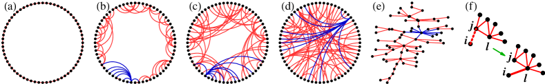
Figure 1: (a)-(d): Example with $N=L=64$, $\bar{k}=2$ at $\alpha=2$. Snapshots after $t$ iterations of the LRM (f), with (a) $t=0$, (b) $t=4N$, (c) $t=12N$ and (d) $t=N^{2}$. Blue (darker in gray scale) links meet at the node with the highest degree. (e): Different layout of (d). (f): LRM described in the text.

In this paper we address the particular problem of whether SFN’s can arise from mechanisms excluding both PA and growth. Recent works lassig ; bauer ; burda proposed theories of networks at equilibrium. In some of these cases bauer ; burda a SFN can be generated simply by choosing the desired degree distribution to be SF. On the other hand, different works obtained SFN without plugging in an a priori degree distribution caldarelli ; valverde ; doye ; hidden . In the spirit of the latter strategy, we propose an example of equilibrium network with Hamiltonian that can yield hierarchical SFN’s. The energy function depends on the degrees of the nodes and of their neighbors lassig . Since it favors connections between nodes with degrees as different as possible, it leads to networks with disassortative mixing assort . Furthermore, the simulation is implemented by using a local rewiring rule. Dynamics of this kind appear natural for biological networks, which indeed are disassortative assort ; maslov . In particular, in food webs we expect each species to find not convenient to interact with similar (and competing) ones. We notice that in food webs both exponential and SFN’s are found food , as we have in our model.

We consider a connected network, represented by a single component undirected graph, composed of $N$ nodes connected by $L$ undirected links (edges). The network topology is uniquely determined by its adjacency matrix ${\bf c}$, such that $c_{ij}=1$ if nodes $i$ and $j$ are linked, and $0$ otherwise. The degree of a node $i$ is indicated as $k_{i}=\sum_{j\neq i}c_{ij}$. We define an energy associated with a link between the $i$-th and the $j$-th nodes having the following form:

$$\epsilon_{ij}=-c_{ij}\left(1-\frac{\min\{k_{i},k_{j}\}}{\max\{k_{i},k_{j}\}}\right)\,.$$ (1)

This equation implies that the energy of a link decreases with the difference in nodal degrees at the two ends of the link and it contributes no energy when the link connects two nodes of same degrees. The Hamiltonian of a network configuration ${\mathcal{G}}$ is then

$$H(\mathcal{G})=\sum_{i<j}\epsilon_{ij}\,.$$ (2)

To generate the initial connected network we first add $L_{0}=N$ links to form a graph with the topology of a ring (see Fig. 1(a)). The remaining $L-L_{0}$ links are added sequentially and randomly, to connect unlinked nodes. The network is evolved by using a local rewiring move (LRM), depicted in Fig. 1(f). A set of three nodes is randomly selected. First, a node $i$ is selected with probability $1/N$, secondly the node $j$ which is a neighbor of $i$ is selected with probability $1/k_{i}$ and finally the node $l\neq i$ which is a neighbor of $j$ is selected with probability $1/(k_{j}-1)$. If $c_{il}=0$, a LRM attempts to delete the $i$-$j$ link of the graph ${\cal G}$ and introduce the $i$-$l$ link to obtain the new graph ${\cal G}^{\prime}$ with a probability

$$p=\min\left\{1,e^{-\alpha[H({\mathcal{G}^{\prime}})-H({\mathcal{G}})]}\right\}\,,$$ (3)

where $\alpha$ is a tunable parameter. For $\alpha=0$ the LRM is always accepted cm03 . In this case the difference between the typical graphs and RG’s is reflected in the degree distribution. Using a master equation approach baiesi , one can show that the degree distribution $P(k)$ indeed decays exponentially, as shown numerically in Fig. 2. In the opposite limit of $\alpha\to\infty$, LRM strongly favors connecting nodes with degrees as different as possible. As a result, usually graphs have several high degree nodes (hubs) connected to many other mono-degree nodes (leaves). Notice that the LRM cannot split the network in disjoint components.

The probability (3), the introduction of the Hamiltonian (2) and the LRM have been chosen for their simplicity and for their analogy with usual rules of equilibrium statistical mechanics, but they do not yield an equilibrium distribution of (2) at an inverse temperature $\alpha$. However, one can see that the above implementation gives the canonical distribution of configurations with weights $\prod_{i=1}^{N}(k_{i}-1)!\,e^{-\alpha H(\mathcal{G})}$, hence allowing a description of the system in terms of ensemble of connected networks at the equilibrium given by the Hamiltonian $H_{\rm eq}(\mathcal{G})\equiv-\alpha^{-1}\sum_{i=1}^{N}\ln(k_{i}-1)!+H(\mathcal{G})$, at temperature $\alpha^{-1}$. Thus, $H(\mathcal{G})$ can be thought as an interaction term from which we expect the arising of complex correlations in the network. Due to $H(\mathcal{G})$, the fraction of second neighbors of the node $i$ represented by the first neighbors of node $j$ and of node $l$ (in the LRM, Fig. 1(f)) belongs to the subset of nodes contributing to the energy balance in a LRM. The non-trivial build up of the correlations necessary to obtain SFN’s should require $\gamma<3$, meaning an average number of second neighbors $\sim N$. On the contrary, $\gamma>3$ would forbid the LRM to “feel” the global structure of the network, hardly giving a fine self-tuning of the network correlations. As shown below, indeed we find SFN’s with $2<\gamma<3$.

We apply the described dynamical rules to networks composed by $N$ up to $8192$ nodes and $L=N\overline{k}/2$, where the average degree $\overline{k}$ is fixed. Thus, we consider sparse networks in the limit of large $N$, where the number of links $L$ is much smaller than the maximum number $L^{\rm max}_{N}=N(N-1)/2$ of possible links in a $N$-clique. This is motivated by the case of most of the real networks, where typically a link between two nodes is an expensive or rare object. In our case, we have mainly used $\overline{k}=4$, such that $L=2N$.

After a large number $\tau\approx 2N^{2}$ of LRM attempts on the initial configurations with $\overline{k}=4$, we observe a significant reorganization of the entire network structure. For $t\gtrsim\tau$ iterations of the LRM, equilibrium is reached, as indicated by the stable shape of the distribution $P_{\alpha,N}(k)$ of the degrees (see Fig. 2). The most interesting region is $0.8\lesssim\alpha\lesssim 4.0$, where $P_{\alpha,N}(k)$ appear as power laws. By increasing $\alpha$, their slopes decrease and their shape changes at large $k$’s, where a shoulder grows, indicating the enhanced tendency in the network to form hubs, as expected. For $\alpha\gtrsim 4.0$ the fraction of hubs is even more consistent and the shoulder at high degrees in the $P_{\alpha,N}(k)$ is substituted by a bump (see for instance the curve for $\alpha=8$ in Fig. 2). Contrary to other models bianconi , an analysis of the mean degree of the largest hub indicates that here it does not attract a finite fraction of links, for $N\to\infty$.

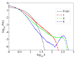
Figure 2: Log-log plot of the degree distributions for $N=4096$, $\overline{k}=4$ and at various $\alpha$’s.

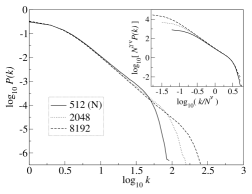
Figure 3: Degree distributions for $\alpha=1$. Inset: distributions rescaled (4) with the $\gamma$ and $\nu$ values quoted in Table 1.

We now focus on the range $0.8\lesssim\alpha\lesssim 4.0$, where the degree distributions are broad and power-law like. To support this SF picture we plot Figure 3, in which a remarkable feature of this model is evident, namely, the self-similar shape of the $P_{\alpha,N}(k)$ for fixed $\alpha$. This is consistent with a finite size form

$$P_{\alpha,N}(k)\simeq k^{-\gamma(\alpha)}f\left(k/N^{\nu(\alpha)}\right)\,,$$ (4)

where $f(x)$ is a scaling function giving a cutoff for sufficiently large values of $x$, and $f(x)\sim{\textit{const}}$ for $x\to 0$. In order to quantify the SF nature of the networks and to support the proposed scaling (4), we perform a finite size analysis, first extrapolating the value of the distributions slope at fixed $\alpha$ and for $N\to\infty$. In Table 1 we show the results. For each $\alpha$, the value of $\gamma$ so obtained is the starting point for attempting a data collapse, by using a rescaling of the form $N^{\gamma\nu}P(k)$ vs ${k/N^{\nu}}$. The values of $\gamma$ that give better collapses (see Table 1) turn out to be close to the extrapolated values, such that the whole picture is consistent. In addition, we note that the data collapses get worse close to the boundaries of the SF region $0.8\lesssim\alpha\lesssim 4.0$, while outside this range we can not make good rescalings. This supports our first, subjective delimitation of the SF region (we stress that the $\overline{k}=4$ case is treated).

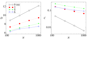
Figure 4: Mean diameter ${\cal D}$ and mean clustering coefficient $C$ as a function of $N$ (linear-log and log-log plot, respectively), for the same set of $\alpha$ values.

Table 1: Numerical evaluation of the exponents of Eq. (4).

$\alpha$	0.8	1	2	3	4
$\gamma$	2.9(2)	2.8(2)	2.4(1)	2.3(2)	2.1(3)
$\gamma$	3.0	2.8	2.3	2.2	2.2
$\nu$	0.4	0.45	0.55	0.58	0.58

It is interesting to examine the other stylized features of networks. In Figure 4 we plot the mean diameter ${\cal D}(N)$ (the maximum of the shortest paths between any nodes of a network) as a function of $\log N$ for the some representative $\alpha$ values. The curves are consistent with a scaling ${\cal D}(N)\sim A+B\log N$ (it seems to be sub-logarithmic cohen for high $\alpha$). Thus, not surprisingly the small world picture is recovered also in our model.

Given a node $i$ connected with $k_{i}$ neighbors, if $m_{i}$ is the number of links between these neighbors, one can quantify the (local) degree of clustering by the clustering coefficient $C_{i}\equiv m_{i}/L^{\rm max}_{k_{i}}$. The mean clustering coefficient $C$ is then the average of the $C_{i}$ over all nodes of all graph realizations at a given $\alpha$. In Figure 4 we also plot $C$ as a function of $N$, in a log-log scale. The plots are compatible with $C\sim N^{-\sigma(\alpha)}$ for $N\to\infty$, with $\sigma$ ranging from $\approx 1$ to $\approx 0.25$ for $0\leq\alpha\leq 6$. For the studied $N$’s, we notice that the highest clustering is found close to $\alpha=4.0$, while it is smaller for high and low $\alpha$.

Our model also shows the power law dependence

$$C(k)\sim k^{-\beta}$$ (5)

indicating that nodes with few links are typically well clustered while hubs hardly are related to high clustering. The concept of modularity was introduced to account for the hierarchical clustering found in many networks ravasz03 ; szabo . In this contexts, networks are built of rather well identifiable clusters, which are themselves composed by clustered subunits, and so on. While in Figure 5 we see that $\beta=0$ for $\alpha=0$, as for RG, for increasing $\alpha$ a scaling (5) takes place in a non negligible interval of $k$, with a $\beta$ raising with $\alpha$ up to values close to $\beta=1$. Hence, in a present issue on whether $\beta=1$ is universal ravasz03 , our result is in favor of the non-universal character of this exponent.

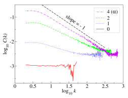
Figure 5: Clustering coefficient as a function of the degree, for four values of $\alpha$ and $N=8192$.

In summary, we have described a static network model with a dynamics favoring networks with disassortative mixing and high clustering, where at least three phases can be identified by increasing the parameter $\alpha$, respectively: exponential, scale free and hub-leaves regimes. The scale free regime has a signature of modularity (the clustering coefficient scales as a power law of the degree with a non-trivial exponent), and the exponent $\gamma$ is comprised in the interesting range $2<\gamma<3$. Thus, many of the characteristics displayed by real networks, usually associated to growing networks with preferential attachment, can be obtained as well in networks with a fixed number of nodes, by using a random rewiring that does not require preferential attachment.

We gratefully acknowledge useful discussions with A. L. Stella. M. B. acknowledges the support of MIUR-COFIN01 and INFM-PAIS02.

References

- (1) P. Erdös and A. Rényi, Publ. Math. Debrecen, 6, 290 (1959).
- (2) D. J. Watts and S. H. Strogatz, Nature, 393, 440 1998; D. J. Watts, Small Worlds: The Dynamics of Networks Between order and Randomness, (Princeton 1999).
- (3) A.-L. Barabási, Linked: The New Science of Networks (Perseus, Cambridge, 2002); S. N. Dorogovtsev and J. F. F. Mendes, Evolution of Networks: From Biological Nets to the Internet and WWW (Oxford University Press, 2003).
- (4) R. Albert and A.-L. Barabási, Rev. Mod. Phys. 74, 47 (2002); S. N. Dorogovtsev and J. F. F. Mendes, Adv. Phys. 51, 1079 (2002); M. E. J. Newman, cond-mat/0303516.
- (5) M. Faloutsos, P. Faloutsos and C. Faloutsos, Proc. ACM SIGCOMM, Comput. Commun. Rev., 29, 251 (1999).
- (6) S. Lawrence and C. L. Giles, Science, 280, 98 (1998); Nature, 400, 107 (1999); R. Albert, H. Jeong and A.-L. Barabási, Nature, 401, 130 (1999).
- (7) The Small World, edited by M. Kochen (Ablex, Norwood, 1989)
- (8) M. E. J. Newman, Proc. Nat. Acad. Sci. 98, 404 (2001).
- (9) E. Ravasz and A.-L. Barabási, Phys. Rev. E67, 026112 (2003).
- (10) A.-L. Barabási and R. Albert, Science, 286, 509 (1999).
- (11) J. A. Dunne and R. J. Williams and N. D. Martinez, Proc. Nat. Acad. Sci. 99, 12917 (2002).
- (12) E. Ravasz et al, Nature 297, 1551 (2002).
- (13) S. Maslov and K. Sneppen, Science 296, 910 (2002).
- (14) Uetz et al, Nature 423, 623 (2000); I. Xenarios et al, Nucl. Acid. Res. 28, 289 (2000); T. Tashiro et al, Proc. Nat. Acad. Sci. 99, 1143 (2000).
- (15) A.-L. Barabási et al., to appear in Sitges Proceedings on Complex Networks, 2004.
- (16) R. V. Solé, R. Pastor-Satorras, E. D. Smith, and T. Kepler, Adv. Complex Syst. 5, 43 (2002); A. Vasquez, A. Flammini, A. Maritan, and A. Vespignani, Complexus 1, 38 (2003).
- (17) J. Berg, M. Lässig and A. Wagner, cond-mat/0207711.
- (18) G. Mukherjee and S. S. Manna, Phys. Rev. E 67, 012101 (2003).
- (19) J. Berg and M. Lässig, Phys. Rev. Lett. 89, 228701 (2002).
- (20) M. Bauer and D. Bernard, cond-mat/0206150.
- (21) Z. Burda and A. Krzywicki, cond-mat/0207020.
- (22) S. Valverde, R. F. Cancho, R. V. Solé, Europhys. Lett. 60, 512 (2002).
- (23) J. P. K. Doye, Phys. Rev. Lett. 88, 238701 (2002).
- (24) G. Caldarelli, A. Capocci, P. De Los Rios, and M. A. Munoz, Phys. Rev. Lett. 89, 258702 (2002).
- (25) M. Boguna and R. Pastor-Satorras, cond-mat/0306072.
- (26) M. E. J. Newman, Phys. Rev. Lett. 89, 208701 (2002).
- (27) For a similar model, see Ph. Blanchard, A. Ruschhaupt, and T. Krueger, cond-mat/0304563.
- (28) M. Baiesi, in preparation.
- (29) G. Bianconi and A.-L. Barabási, Phys. Rev. Lett. 86, 5632 (2001).
- (30) R. Cohen and S. Havlin Phys. Rev. Lett. 90, 058701 (2003).
- (31) G. Szabó, M. Alava and J. Kertész, cond-mat/0208551.