Remarks on homo- and hetero-polymeric aspects of protein folding

Abstract

Different aspects of protein folding are illustrated by simplified polymer models. Stressing the diversity of side chains (residues) leads one to view folding as the freezing transition of a heteropolymer. Technically, the most common approach to diversity is randomness, which is usually implemented in two body interactions (charges, polar character,..). On the other hand, the (almost) universal character of the protein backbone suggests that folding may also be viewed as the crystallization transition of an homopolymeric chain, the main ingredients of which are the peptide bond and chirality (proline and glycine notwithstanding). The model of a chiral dipolar chain leads to a unified picture of secondary structures, and to a possible connection of protein structures with ferroelectric domain theory.

Lectures given at the Trieste Workshop on Proteomics: Protein Structure, Function and Interaction, May 5-16 2003

Saclay T03/051

1 Introduction

Proteins are polymers, which have the property of folding reversibly into a single geometrical shape with biological activity. The folding process can be modeled as a phase transition from a high temperature coil phase to a low temperature compact phase (other parameters, e.g. pH, may also trigger the transition). Both phases require a very detailed description of the monomers, not to mention the chemistry of water. These notes aim at presenting some of the theoretical approaches to the folding transition. The interested reader can find more details in the short list of references at the end of the paper.

Section 2 gives a brief description of the twenty monomers (amino acids) which are the building blocks of proteins. A protein of $N$ amino acids can be characterized by its primary structure, i.e. by specifying which amino acid is actually at position $({\rm i})$ along the chain (with ${\rm i}=1,2...N$ and $N$ of the order of a few hundreds).

At first sight, a protein may be considered as a heteropolymer, with amino acid $({\rm i})$ being characterized by its electric charge $(q_{i})$, its hydrophilicity $(\lambda_{i})$…. A closer look at a protein chain reveals that this heteropolymer is made of an almost periodic backbone and of different side chains (residues). This almost periodic backbone is almost protein independent, leading to a homopolymeric approach to the folding transition. This homopolymeric view is supported by the ubiquitous existence of helices and sheets in proteins (which are called the secondary structures). Folded proteins illustrate the coexistence of specific features (primary sequence, type of biological activity,…) and universal features [1, 2] such as helices and sheets (one may also speculate about the universal character of other issues, such as the very existence of a biological activity or the aggregated structures in amyloid-like diseases [3]).

Some of these properties will be illustrated, mostly in a pictorial way, on a small protein (1aps, $N=98$) in Section 3. This example shows that one is not concerned by the theorists’ thermodynamic limit: proteins have a finite size, pointing towards an important role of the surface, and therefore of the solvent (i.e. water for globular proteins). More numbers pertaining to the folding process will be given in Section 4.

I think it is fair to say that the homopolymeric aspects of proteins have been so far less studied. Since there are numerous reviews on their heteropolymeric properties, I will mostly deal here with homopolymeric models, and conclude on the interplay between both types of properties.

2 Chemistry [1, 2]

• A brief description of the monomers

  • There are twenty different types of monomers ASP, GLU, LYS, ARG, ALA, VAL, PHE, PRO, MET, ILE, LEU, SER, THR, TYR, HIS, CYS, ASN, GLN, TRP, GLY

  • These monomers are amino acids (exception: PRO)

    ${\rm{{\bf H_{2}N}-C_{\alpha}HR-{\bf COOH}}}$

    e.g.

    ALA: ${\rm R=CH_{3}}$

    GLU: ${\rm R=(CH_{2})_{2}-COO^{-}}$

  • The amino acids are chiral (exception: GLY)

    ${\rm{H_{2}N-{\bf C_{\alpha}}HR-COOH}}$

    Sitting on the ${\rm C_{\alpha}-H}$ bond and looking towards the ${\rm C_{\alpha}}$ atom, one sees the ${\rm CO-R-N}$ sequence in a clockwise way.

  • Residues ${\rm R}$ have different properties

    ${\rm{H_{2}N-C_{\alpha}H{\bf R}-COOH}}$

    • Charged residues ASP (-), GLU (-), LYS (+), ARG (+)

    • Polar residues TYR, HIS, ASN, GLN

    • Rather polar residues PRO, THR, ALA, GLY, SER

    • Hydrophobic residues VAL, PHE, MET, ILE, LEU, TRP, CYS

• From monomer to polymer

  • Formation of the peptide bond

    

    Figure 1: Peptide bond: the ${\rm C}_{\alpha}-{\rm C}_{\alpha}$ virtual bond is roughly perpendicular to the CO and NH bonds.

    Geometrical constraints (stemming from quantum chemistry), imply that consecutive ${\rm{{\bf C_{\alpha}}-CO-NH-{\bf C_{\alpha}}}}$ atoms are coplanar, with the C-O (and N-H) bonds being roughly perpendicular to the virtual ${\rm{{\bf C_{\alpha}}-{\bf C_{\alpha}}}}$ bond.

    At long distance, the charge distribution on the peptide bond is dominated, in a first approximation, by an electric dipole parallel to ${\rm{OC}}$ and of order four Debyes. At shorter distances, this charge distribution gives rise to hydrogen bonds.

    With the exception of residues GLY and PRO, the backbone chain can be written ${\rm{...NH-{\bf C_{\alpha}}-CO-NH-{\bf C_{\alpha}}-CO-NH-{\bf C_{\alpha}}-CO-NH-{\bf C_{\alpha}}-CO...}}$

  • Chirality of the main chain

    The chirality of the amino acids, together with the steric constraints gives to the main backbone chain some sort of chirality. More precisely, taking four atoms 1234 along the main backbone chain, the associated dihedral angle $\widehat{1234}$ is defined as the angle of the (123) and (234) planes. It is shown in Figure 2, with the 2-3 bond coming out of the paper. The convention is such that the above dihedral angle $\widehat{1234}$ is negative. Note that $\widehat{1234}=\widehat{4321}$.

    

    Figure 2: Defining the dihedral angle $\widehat{1234}$ for atoms 1,2,3,4

    The chirality of the chain is associated with the fact that positive and negative dihedral angles do not have the same steric constraints and therefore not the same (free) energies. In particular, Ramachandran’s plots for a given residue, are given for $\phi=\widehat{1234}$ (resp. $\psi$) where $1234={\rm CNC_{\alpha}C}$ (resp. $1234={\rm NC_{\alpha}CN}$). Except for GLY, these plots show that helices and sheets correspond to rather well defined (and non symmetric) regions in $\phi,\psi$ space.

    One may also define Ramachandran’s plots for side chains, but we will neglect their role in this paper.

  So with the (important) exceptions of residues GLY and PRO, the main backbone chain can be represented in a homopolymeric way (see e.g. [4]). One may then consider the chiral (hydrogen-bonding+dipolar) chain as a good description of secondary structures in proteins.

3 Example

I will illustrate some of the previous points on a specific protein (1aps).

• Primary structure ( $N=98$ residues)

  (i=1) SER-THR-ALA-ARG-PRO-LEU-LYS-SER-VAL-ASP-TYR-GLU-VAL-

  -PHE-GLY-ARG-VAL-GLN-GLY-VAL-CYS-PHE-ARG-MET-TYR-ALA-

  -GLU-ASP-GLU-ALA-ARG-LYS-ILE-GLY-VAL-VAL-GLY-TRP-VAL-

  -LYS-ASN-THR-SER-LYS-GLY-THR-VAL-THR-GLY-GLN-VAL-GLN-

  -GLY-PRO-GLU-GLU-LYS-VAL-ASN-SER-MET-LYS-SER-TRP-LEU-

  -SER-LYS-VAL-GLY-SER-PRO-SER-SER-ARG-ILE-ASP-ARG-THR-

  -ASN-PHE-SER-ASN-GLU-LYS-THR-ILE-SER-LYS-LEU-GLU-TYR-

  -SER-ASN-PHE-SER-VAL-ARG-TYR (i=98)

  

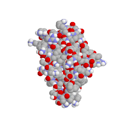
  Figure 3: Native spacefilled structure of 1aps

  

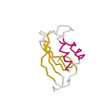
  Figure 4: Backbone of 1aps: Helices 1 (PHE 22-ILE 33) and 2 (GLU 55-LEU 65). Sheet ( strand 1 (LYS 7-VAL 13); strand 2 (VAL36-THR 42); strand 3 (THR 46-GLY 53); strand 4 (ARG 77-THR 85); strand 5 (ASN 93-ARG 97))

• Compactness of the folded structure (Figure 3)

  The total number of atoms is of order one thousand, linking protein folding with cluster physics (with a chain constraint) [5, 6].

• Charged residues (Figure 5)

  There are 26 charged residues (three ASP, seven GLU, seven ARG and nine LYS). For electrostatic reasons, they are located on the protein surface. More generally, since there are four (out of twenty) charged residues in usual conditions, and assuming equipartition, a protein of N residues has N/5 charged residues to be placed on the surface (which scales likes $N^{2\over 3}$), leading to an estimate $N\sim 125$ for a typical single domain protein.

• The main backbone chain (Figures 4, 6, 7)

  As mentioned above, the main chain is homopolymeric with the exception of three PRO and eight GLY residues. This homopolymeric character is illustrated by the CO bonds. The (roughly) ferroelectric order of helices and the (roughly) antiferroelectric character of sheets result from hydrogen bonding and dipolar-like forces.

  

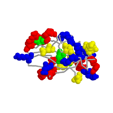
  Figure 5: Charged residues of 1aps

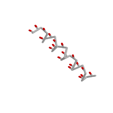
Figure 6: Homopolymeric backbone: CO bonds of a helix

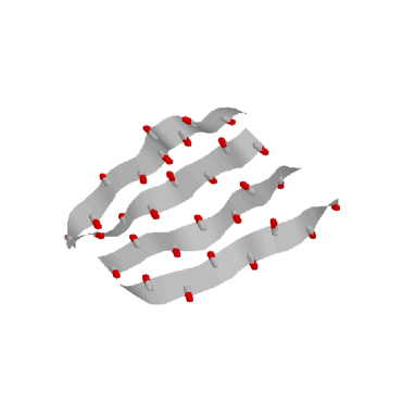
Figure 7: Homopolymeric backbone: CO bonds of a sheet

I could not find the active site of 1aps on the web. From a physical point of view, one would like to understand how the primary sequence somehow encodes the native structure (to further extract the active site from the native structure is not easy).

4 Numbers [1, 2]

• Energy scales

  At room temperature ${\rm T_{0}}$, the equivalence between chemical and physical units is ${\rm{k_{B}T_{0}}}\sim 0.6\ {\rm{kcal/mole}}\sim{1\over 40}\ {\rm{eV/part}}$. A hydrogen bond has an energy of order 2-6 kcal/mole. A covalent bond has an energy of order $50-200$ kcal/mole. In the folded state, two consecutive peptide bonds have an energy of order 1-3 kcal/mole ( obtained from ${p_{0}^{2}\over 4\pi\epsilon_{0}\epsilon_{r}d^{3}}$, with $p_{0}\sim 4$ Debyes, $d\sim 4$ Å, and where $\epsilon_{r}$ is believed to be of order $2-5$). Finally, van der Waals attraction energies are of order 0.3-1 kcal/mole.

  The folding transition is first order, with an entropy loss of order $k_{B}$ or less per residue (possibly raising questions on the applicability of Classical Statistical Mechanics).

  The dynamics of the folding is governed by energy barriers: the range of folding times is of order $10^{-3}-1s$, and even longer; it should be compared with microscopic times of order $10^{-13}-10^{-15}s$. This suggests that the phase space of a protein may have many trapping local minima, implying problems in numerical simulations.

• Geometry and Energy

  A typical protein has something like $N\sim 100-500$ residues (the number of atoms being of order a few thousands). Something like half of the residues belong to the surface. A typical linear size of the folded molecule is $R\sim 50$ Å. As can be seen from the examples of 1aps and other proteins, the typical length of a helix is 10-20 residues, that of a strand being smaller (may be 5-8 residues). In broad terms, proteins are clusters-with-a chain-constraint (and a solvent). Geometrical constraints (bond lengths, valence angles, van der Waals radii, chirality,..) play an important role in proteins. The all-atom CHARMM energy $E$ commonly used in numerical situations is given by [7]

  $$E=\sum_{{\rm bonds}}k_{b}\left(b-b_{0}\right)^{2}+\sum_{{\rm angles}}k_{\theta}\left(\theta-\theta_{0}\right)^{2}$$

  $$+\sum_{{\rm dihedrals}}k_{\phi}(1+{\rm cos}(n\phi-\delta))+\sum_{{\rm impropers}}k_{\nu}\left(\nu-\nu_{0}\right)^{2}$$

  $$+\sum^{\ \ \ \ \ \prime}_{i<j}4\varepsilon_{ij}\left\{\left({\sigma_{ij}\over r_{ij}}\right)^{12}-\left({\sigma_{ij}\over r_{ij}}\right)^{6}\right\}+\sum^{\ \ \ \ \prime}_{i<j}{332\over\varepsilon_{r}}{q_{i}q_{j}\over r_{ij}}$$

  (1)

  where distances are in Angströms, angles in radians and $E$ in ${\rm kcal/mol}$. Studying the dielectric permittivity $\varepsilon_{r}$ is a difficult task; it is believed to be of order $2-5$ in a folded protein.

• (Bio)chemistry

  Before considering simplified models, let me recall a few facts about real proteins. One should be cautious about in vivo vs in vitro folding (role of chaperone molecules). Real proteins are not random polymers, but have been evolution selected. Since (quantum) hydrogen bonds are important in proteins, the use of Classical Statistical Mechanics may be questioned. To this discouraging list, one may add that water (for globular proteins) is a complicated, strongly structured solvent. We will not even mention the biochemical activity (e.g. the recognition of the active site by a ligand). The distance between real proteins and simplified models is not to be underestimated.

5 Simplified models: homopolymeric approach

5.1 Modeling hydrogen bonds in a compact phase

The discovery of helices and sheets by Pauling and Corey [8, 9] relies on the existence of short range hydrogen bonds. Let us consider first an all-helix folded protein. What we have here is a competition between local and global orders: the former favors helical (i.e. one dimensional) structures (figure 8), whereas the latter favors compact (i.e. three dimensional) structures.

This competition can be modeled as follows. We consider a polymer chain on a cubic lattice, where the monomers interact with an attractive van der Waals energy $\varepsilon_{v}$ (to ensure compactness at low temperature), and a curvature energy $\varepsilon_{h},$ which favors the alignment of two consecutive monomers. In this model, a monomer represents a helical turn of the protein (two consecutive helical turns allowing for the presence of hydrogen bonds).

The phase diagram depends on the ratio $({\varepsilon_{v}\over\varepsilon_{h}})$; for simplicity, we will restrict the discussion to fully compact structures ($\varepsilon_{v}=\infty$). The case $\varepsilon_{h}=0$ is of interest in the physics of hydrophobic chains at temperature below the $\theta$ point, which are known to possess a large entropy in the compact phase. We will first study this model, and then consider the influence of the curvature term $\varepsilon_{h}$. Technical details are postponed to an Appendix.

Figure 8: Hydrogen bonds in a helix

5.1.1 Entropy of a hydrophobic chain [10]

We first define a Hamiltonian Path (HP) as a fully compact self avoiding walk (SAW). The number of Hamiltonian Paths (HP) on the lattice is formally described by

$${\cal N}_{N}=\sum_{(HP)}{\bf 1}$$

Introducing an n-component field $\vec{\varphi}_{\vec{r}}$ at each point $\vec{r}$ of the lattice, and using the properties of the limit $n\to 0$, it is shown in the Appendix that

$${\cal N}_{N}={\rm lim}_{{\rm n}\to 0}{1\over{\rm n}}\int{\cal D}{\vec{\varphi}_{r}}\ e^{-{1\over 2}\sum_{(r,r^{\prime})}{\vec{\varphi}}_{r}\ (\Delta^{-1})_{{\vec{r}}{\vec{r}^{\prime}}}\ {\vec{\varphi}}_{r^{\prime}}}\prod_{r}\left({1\over 2}{\vec{\varphi}_{r}}^{2}\right)$$ (2)

where $\Delta_{{\vec{r}}{\vec{r}^{\prime}}}=1$ if $\vec{r}$ and $\vec{r}^{\prime}$ are nearest neighbour sites, and $0$ otherwise.

A homogeneous and isotropic saddle point evaluation $\vec{\varphi}_{\vec{r}}=\vec{\varphi}$ yields

$${\cal N}_{N}=\left({q\over e}\right)^{N}$$ (3)

with $q=2d=6$.

This calculation suggests that a collapsed homopolymeric chain is a mixture of an exponentially large number of conformations, and is therefore not able to describe the single conformation of a native protein. For this reason, the folding transition is commonly thought to be quite different from the $\theta$ transition. Note however that equation (3) depends on the use of a homogeneous saddle point in equation (2), which is consistent with the use of periodic boundary conditions. More general boundary conditions (corresponding to non-homogeneous $\vec{\varphi}_{\vec{r}}$) would give a expression of the form

$${\cal N}_{N}\sim A\mu^{N}\ {\widetilde{\mu}}^{N^{2/3}}$$ (4)

where $A$ is a constant, $\mu$ and $\widetilde{\mu}$ being respectively bulk and surface connectivities.

5.1.2 “Helices” in a compact phase

We now implement the competition between one- and three-dimensional structures, by introducing a curvature energy $\varepsilon_{h}$. As mentioned above, this curvature energy favors aligned consecutive “monomers” (or disfavors corners in the HP). Denoting by $N_{corners}(HP)$ the number of corners in a given (HP), the number of weighted (HP) is given by

$${\cal N}_{h}=\sum_{(HP,corners)}e^{-\beta N_{corners}(HP)\varepsilon_{h}}$$

where the summation runs over all possible (HP)’s and over all possible corners, and where $\beta={1\over T}$ is the inverse temperature.

Introducing $d$ ${\rm n}$-dimensional fields: ${\vec{\varphi}}_{\alpha r}$ , $\alpha=1,2,...d$ for each lattice site $(r)$, it is shown in the Appendix that

$${\cal N}_{h}={\rm lim}_{{\rm n}\to 0}{1\over{\rm n}}\int{\cal D}{\vec{\varphi}}_{\alpha r}\ e^{-{1\over 2}\sum_{\alpha=1}^{d}\sum_{(r,r^{\prime})}{\vec{\varphi}}_{\alpha r}\ (\Delta_{\alpha}^{-1})_{{\vec{r}}{\vec{r}^{\prime}}}\ {\vec{\varphi}}_{\alpha r^{\prime}}}\prod_{r}\left({1\over 2}\sum_{\alpha=1}^{d}{\vec{\varphi}}_{\alpha r}^{2}+e^{-\beta\varepsilon_{h}}\sum_{\alpha<\gamma}{\vec{\varphi}}_{\alpha r}\cdot{\vec{\varphi}}_{\gamma r}\right)$$ (5)

where $\Delta^{\alpha}_{\vec{r}\vec{r}^{\ \prime}}$ is 1 if $\vec{r}$ and $\vec{r}^{\ \prime}$ are nearest neighbours in direction $\alpha$ and $0$ otherwise.

Performing a homogeneous and isotropic saddle point in equation (5) we get

$${\cal N}_{h}=\left({q(\beta)\over e}\right)^{N}$$ (6)

with an effective coordination number, $q(\beta)=2+2(d-1)e^{-\beta\varepsilon_{h}}$.

A first order crystallization transition, describing the competition between the entropy gain of making turns, and the corresponding energy loss, occurs for $q(\beta_{c})=e$. For $d=3$, the transition temperature is $k_{\rm B}T_{c}=0.58\ \varepsilon_{h}$. Below the transition, the entropy is not extensive. The average length of a helix is given by

$$\ell={N\varepsilon_{h}\over U\left(\beta_{c}\right)}$$

where $U(\beta)=-{\partial\over\partial\beta}{\rm log}\ {\cal N}_{h}$ is the internal energy. Just above the transition, in $d=3,$ the average helix length is equal to $\ell_{c}=3.78$, and is of ${\cal O}(\ell=N^{1/3})$ in the low temperature phase. Note that in this very simplified picture $\ell_{c}$ corresponds to a typical number of residues of the order of 15, since one monomer corresponds to a helical turn, that is 3.6 residues. As seen from the example of 1aps, and from numerical calculations using Hamiltonians such as (equation(1)), this is indeed the typical length of $\alpha$-helices in proteins.

These results result from a homogeneous saddle point assumption (implying the use of periodic boundary conditions). In a more correct treatment, we expect a non extensive surface entropy of order $N^{2\over 3}$ in the crystalline phase (corresponding to the fact that the corners are on the surface of the lattice). The influence of boundary conditions on the counting of (HP), with or without curvature energy, is a rather difficult subject [11].

Finally, relaxing the constraint ($\varepsilon_{v}=\infty$), yields a phase diagram where one may reach the crystallized phase either through a $\theta$ transition followed by a second (liquid globule-crystal) transition, or through a unique discontinuous coil-crystal transition [12]. One may thus consider that there are two coil “phases”, one above the $\theta$ transition, and the other above the crystallization transition, differing by their short range order.

5.1.3 Fully compact “sheets”

The extension to sheets (see figure 9) can be done with a slight generalisation of the Hamiltonian Path formalism: a node of a path is now to be interpreted as an amino acid.

Figure 9: Hydrogen bonds in a sheet

The model can be described in the following way. Consider a Hamiltonian path. To mimic the formation of ${\rm CO-HN},$ i.e. a hydrogen bond (H-bond), in $\beta$-sheets, we allow an ${\rm H}$-bond (energy gain $\varepsilon_{s}),$ whenever two pairs of aligned links belong to two (non intersecting) neighbouring strands. We do not make any distinction between parallel and antiparallel sheets. Following the representation of the Appendix, and performing an isotropic homogeneous saddle point, one also gets a first order crystallization transition. The physics is very similar to the cas of helices. Typical lengths of ordered strands are however more difficult to estimate [13].

5.1.4 Conclusion on Hamiltonian Paths

We have presented a simple model of the formation of secondary structures in a dense phase, which is linked to polymer melting theory. Starting from the coil state, one can reach the “compact state with secondary structures” either directly or through other compact phase(s). These results rest on a homogeneous saddle point approximation, which corresponds to periodic boundary conditions. The “$n\to 0$” approach [14, 15] represents the chain via a field $\vec{\varphi}_{r}$ and is therefore not appropriate to the description of heteropolymeric properties ( where the information depends of the curvilinear abcissa $(i)$ along the chain). In our presentation, helices and sheets were treated on a different footing, since one monomer was a helical turn (3.6 amino acids) in the former case or a single amino acid in the latter. This dissymetry will be corrected below where we also consider the long range contribution of the dipole-dipole interaction.

5.2 The dipolar chain

Since the peptide bond has a large dipole moment, it seems rather natural to investigate the properties of the dipolar chain, which connects successive ${\rm C}_{\alpha}$ carbon atoms. Representing the peptide bond by a dipole moment is an approximation, and the dipolar interaction should be modified at short distances. The Hamiltonian of the model then reads

$$\beta{\cal H}={v_{0}\over 2}\sum_{i\neq j}\delta(\vec{r}_{i}-\vec{r}_{j})+{\beta\over 2}\sum_{i\neq j}\sum_{\alpha,\gamma}p_{i}^{\alpha}G_{\alpha\gamma}(\vec{r}_{i},\vec{r}_{j})p_{j}^{\gamma}$$ (7)

In equation (7), $\beta={1\over T}$ is the inverse temperature, $v_{0}$ is the excluded volume, $\vec{r}_{i}$ denotes the spatial position of monomer $i$ ($i=1,2,...N$), and $\vec{p}_{i}$ its dipole moment. If necessary, three body repulsive interactions may be introduced, to avoid collapse at infinite density. The (infinite range) dipolar tensor reads

$$G_{\alpha\gamma}(\vec{r},\vec{r}^{\prime})=A{1\over|\vec{r}-\vec{r}^{\prime}|^{3}}(\delta_{\alpha\gamma}-3v_{\alpha}v_{\gamma})$$ (8)

with $v_{\alpha}={(\vec{r}-\vec{r}^{\prime})_{\alpha}\over|\vec{r}-\vec{r}^{\prime}|}$ and $A$ is a prefactor containing the dielectric constant of the medium. The dipolar interaction (8) is modified at small distances ($|\vec{r}-\vec{r}^{\prime}|<a$) and may also be cut-off at large distances by an exponential prefactor. The partition function of the model (7) is given by:

$${\cal Z}=\int\prod_{i}d{\vec{r}_{i}}d{\vec{p}_{i}}\ {\delta(|{\vec{r}_{i+1}-{\vec{r}_{i}}}|-a)}\ \delta(|{\vec{p}_{i}}|-p_{0})\ \delta(\vec{p}_{i}\cdot(\vec{r}_{i+1}-\vec{r}_{i}))\ \exp\left(-\beta{\cal H}\right)$$ (9)

In equation (9), $a$ denotes the Kuhn length of the monomers, and $p_{0}$ is the magnitude of their dipole moment. The third $\delta$-function constraints the dipole moment $\vec{p}_{i}$ to be perpendicular to the chain (Figure 1), with full rotation around bond $(i,i+1)$.

Apart from numerical simulations, there are two main approaches to the dipolar chain:

(i) one may try to integrate out the dipoles, and get an effective Hamiltonian for the chain. Since dipoles favor anisotropic configurations, one expects that the above orthogonality constraint will lead to an anisotropic collapsed phase.

(ii) one may tackle the full problem, and using what is known about ferroelectric domains, one may guess low energy structures.

The latter approach is not without risks, since the determination of domain structures from first principles is an unsolved problem in non-soft condensed matter physics. The former, which is a little more tractable, is an extension of the hydrogen bond models (see section 5.1), with one important difference: the long range character of the dipole interaction, implies that the surface of the collapsed globule is itself a variational parameter. It also allows for a first step in accounting for chirality.

5.3 Integrating the dipoles

• Order parameters

  For simplicity, we soften the constraint of fixed length dipoles in equation (9) and replace it by a Gaussian constraint. We therefore have

  $${\cal Z}_{G}=\int\prod_{i}d{\vec{r}_{i}}d{\vec{p}_{i}}\ {\delta(|{\vec{r}_{i+1}-{\vec{r}_{i}}}|-a)}\ {1\over({2\pi p_{0}^{2}})^{3/2}}\ e^{-{{\vec{p}_{i}}^{2}\over{2p_{0}^{2}}}}\ \delta(\vec{p}_{i}\cdot(\vec{r}_{i+1}-\vec{r}_{i}))\ \exp\left(-\beta{\cal H}\right)$$ (10)

  where the subscript G on the partition function stands for Gaussian and the Hamiltonian ${\cal H}$ is given by equation (7). Using the identity

  $$\delta(\vec{y})=\lim_{\lambda\to\infty}\left(\lambda\over{2\pi}\right)^{3/2}e^{-{\lambda{\vec{y}}^{2}\over 2}}$$ (11)

  we may now perform the (Gaussian) integrals over the dipole moments $\vec{p}_{i}$ in equation (10). As a result, the problem now depends only on the polymeric degrees of freedom. Introducing the tensorial parameter $Q_{\alpha\beta}(\vec{r})$ by

  $$Q_{\alpha\beta}(\vec{r})=\sum_{i}\left({(\vec{u}_{i})_{\alpha}(\vec{u}_{i})_{\beta}}-\delta_{\alpha\beta}\right)\ \delta(\vec{r}-\vec{r}_{i})$$ (12)

  where $(\alpha,\beta=x,y,z)$ and the notation $\vec{u}_{i}=(\vec{r}_{i+1}-\vec{r}_{i})/a$ was used, we can express the effective Hamiltonian as a function of the physical order parameters

  $$\rho(\vec{r})=-{1\over 2}\ {\rm Tr}\ {\bf Q}(\vec{r})=\sum_{i}\delta(\vec{r}-\vec{r}_{i})$$ (13)

  and

  $$q_{\alpha\beta}(\vec{r})=\sum_{i}(u_{i}^{\alpha}u_{i}^{\beta}-{\delta_{\alpha\beta}\over 3})\ \delta(\vec{r}-\vec{r}_{i})$$ (14)

  In a way analogous to the previous section, the density $\rho(\vec{r})$ is appropriate for an isotropic $\theta$ transition, and the dielectric tensor ${\bf q}(\vec{r})$, is appropriate for a (liquid) crystalline order. Using non rigorous approximations (which are actually valid in a melt), we find that the dipolar chain undergoes a second order $\theta$ transition from the coil phase to a (liquid) collapsed phase, with order parameter $\rho(\vec{r})$, followed, at lower temperature, by a first order transition with order parameter ${\bf q}(\vec{r})$. The ordered phase is a (liquid crystal) collapsed phase.

• Trying to include chirality

  If one follows liquid crystalline traditions [16], chirality is usually represented as the simplest non trivial term in a Landau-like expansion of the free energy in the order parameter ${\bf q}(\vec{r})$. It is well known that chirality is not easy to take into account at a microscopic level [17], but at a Landau free energy level, symmetry considerations lead, to lowest order, to a chiral contribution

  $${\cal F}_{chiral}(\vec{r})=\int\ D\ \epsilon_{\alpha\mu\nu}q_{\alpha\delta}\partial_{\mu}q_{\nu\delta}\ d^{3}r$$ (15)

  where $\epsilon_{\alpha\mu\nu}$ the completely antisymmetric tensor and $D$ is a measure of the strength of the chirality (in fact several parameters are in general needed).

  Using the same non rigorous approximations as above, we find that the $\theta$ transition is very weakly $D$-dependent, whereas the transition towards the liquid crystalline phase increases strongly with $D$ [18]. This liquid crystalline phase is now modulated, and has strong similarities with the liquid crystalline blue phase(s). Interestingly enough, for strong enough chirality, we get a direct transition from a coil phase to a compact phase with a modulated order parameter ${\bf q}(\vec{r})$. More specifically, one has

  $$q_{\alpha\beta}(\vec{k})=\sum_{i}e^{-i\vec{k}\cdot\vec{r}_{i}}(u_{i}^{\alpha}u_{i}^{\beta}-{\delta_{\alpha\beta}\over 3})$$ (16)

  in Fourier space (with $\vec{k}\neq\vec{0}$). The indices $\alpha,\beta$ are space, not replica, indices. The order parameter is very similar for the case of (idealized) helices and sheets where

  (i) a (ideal) helix is described by $\vec{r}_{i}=(u\ {\rm cos}\ v_{i},u\ {\rm sin}\ v_{i},v_{i})$ and constant $u$.

  (ii) a (ideal) sheet is described by $p=1,2,...M$ strands where each strand is described by a segment $\vec{r}_{p}=(u\ {\rm cos}\ v_{p},u\ {\rm sin}\ v_{p},v_{p})$ and constant $v_{p}$.

  To summarize, we have found that within certain models and approximations, we may get for the dipolar chiral chain, a direct and discontinous transition from a coil phase to a compact phase with secondary structures. The order parameter (16) describes both helix-like and sheet-like conformations.

  This model may seem oversimplified. For instance, the chiral term (15) can be rewritten as $\sum_{i,j}\left({\vec{\nabla}}f(\vec{r}_{ij})\cdot(\vec{u}_{i}\times\vec{u}_{j})\right)(\vec{u}_{i}\cdot\vec{u}_{j})$, where $f(\vec{r}_{ij})$ describes a short range (in space) interaction (the coordinates $\vec{r}_{i}$ are the coordinates of the virtual ${\rm C}_{\alpha}$ chain). This term does not compare well to the dihedral terms of the all atom CHARMM energy which read

  $$\sum_{{\rm dihedrals}}k_{\phi}(1+{\rm cos}(n\phi-\delta))$$

  where $\phi(1234)={\rm cos}^{-1}(\vec{n}_{123}\cdot\vec{n}_{234})$ where $\vec{n}_{abc}$ is the unit normal vector to the plane (a,b,c). Our modeling of chirality, through a single parameter and a first order gradient term, is rather primitive. In particular, higher order gradient terms, describing shorter distances, are certainly important (see the example of the blue fog in liquid crystalline blue phases) [19]. Furthermore, the precise spatial organization of the compact ordered phase also depends on its surface.

With all these caveats, it should be mentionned that computing and diagonalizing ($q_{\alpha\beta}(\vec{r})$) for real proteins, leads to a reasonable characterization of secondary structures. Helices are essentially uniaxial (two different eigenvalues), whereas sheets are biaxial (three different eigenvalues) [20].

5.4 Non integrating the dipoles

The non integration of dipoles leads one to consider low energy dipolar structures. I will first recall a few facts on ferroelectric domains (structure, order parameter,…). More speculative issues, such as a “biological” interpretation of defects of this order parameter, or the introduction of surfaces in protein folding, will be briefly examined.

• Dipolar ordering

  There is another way to consider the dipolar Hamiltonian, namely to use the identity (see equation (8))

  $${(\delta_{\alpha\gamma}-3v_{\alpha}v_{\gamma})\over|\vec{r}-\vec{r}^{\prime}|^{3}}={\partial^{2}\over\partial r_{\alpha}\partial r^{\prime}_{\gamma}}\left({1\over|\vec{r}-\vec{r}^{\prime}|}\right)$$ (17)

  Defining a local polarization $\vec{\rm P}(\vec{r})=\sum_{i}\vec{p}_{i}\delta(\vec{r}-\vec{r}_{i})$, one may transform the dipolar term of equation (7) into a Coulomb Hamiltonian, with a (continuous) distribution of bulk ($\rho(\vec{r})=-{\rm div}\ \vec{\rm P}(\vec{r})$) and surface ($\sigma(\vec{r}_{s})=\vec{\rm P}(\vec{r}_{s})\cdot\vec{\rm N}(\vec{r}_{s})$) charges, where $\vec{r}_{s}$ belongs to the surface, and $\vec{\rm N}(\vec{r}_{s})$ is the normal to the surface at this point. Given the dimensions and discreteness of the system, this continuum picture may not be very satisfactory [21], but we will nevertheless use it.

  A (low temperature) collapsed dipolar chain, if long enough, will break into (Bloch, Weiss, Néel…) domains, as I now show on a simple example. Let us consider an Ising chain, with short range exchange $(J_{0})$ interactions between neighbouring monomers (see the Appendix and reference [23]). At low temperature, the chain is collapsed and has a uniform polarization. If one adds a long range dipole-dipole interactions $(J_{dd})$, one may test the stability of the uniform state: flipping half of the dipoles results in an energy cost of order $\Delta E=+J_{0}R^{2}-J_{dd}R^{3}$, where we have considered a spherical globule of radius $R$, and dropped some numerical constants. For $R>R^{\star}={J_{0}\over J_{dd}}$ (or $N>N^{\star}=({J_{0}\over J_{dd}})^{3}$), the system will break into domains.

  For many dipolar systems, low energy domain structures in ferroelectricity (and ferromagnetism) tend to have $\rho(\vec{r})=-{\rm div}\ \vec{\rm P}(\vec{r})=0$ (pole avoidance “principle” [22] ). This “principle” is obeyed in the case of helices (where $\vec{\rm P}(\vec{r})$ is a constant vector) and sheets ( where $\vec{\rm P}(\vec{r})$ has roughly antiferroelectric order). One may understand in a similar way solenoidal proteins (where $\vec{\rm P}(\vec{r})$ looks like a curl, i.e. has a circulating pattern) such as $\beta$-barrels or protein 1a4y (Figure 10).

  

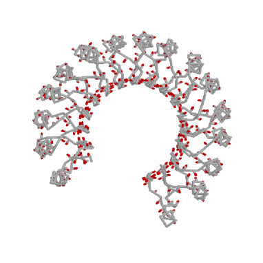
  Figure 10: Circulating CO dipoles in protein 1a4y

  The fact that dipolar interactions couple the $\vec{r}_{i}$’s and the $\vec{p}_{i}$’s implies that dipolar systems are very sensitive to the geometry. For instance, the infinite simple cubic and face centered cubic lattices do not have the same ground state order. For finite systems, the situation is even more tricky, since dipolar interactions “feel” the surface of the system. The formation of domains results in general from the competition between dipolar- and other (shorter range) - interactions. The full determination of domain structures (size, order parameter, spatial organization,…) in non-soft condensed matter physics depends on non-extensive terms in the free energy, and remains an unsolved problem [22].

  At a smaller (cluster) scale, Singer and coworkers [24] have studied the ground state of some dipolar clusters without the chain constraint. They pointed out that possible order parameters are the vectorial spherical harmonics (VSH) [25], and that circulating patterns have then simple expressions. Writing

  $$\vec{\rm P}(\vec{r})=\sum_{(JM)}\sum_{L}A_{JL1}^{M}(r)\vec{Y}_{JL1}^{M}(\theta,\phi)$$

  one may follow what has been done [26] for (scalar) bond orientational order in clusters. In this case, one expands the density as

  $$\rho(\vec{r})=\sum_{(LM)}Q_{LM}(r)Y_{LM}(\theta,\phi)$$

  where the $Y_{LM}(\theta,\phi)$ are the ordinary spherical harmonics. The (VSH) formalism is rather heavy, and I have done only preliminary calculations on real proteins. As expected, helices are easier to analyze than sheets.

• Speculations on order parameters and defects

  One may also wonder whether the existence of an order parameter may help us to understand the existence of an active site, see e.g. [27, 28]. The simplest idea I can think of is to view the active site as a defect of this order parameter (see e.g. [29, 30]). By defect, I mean here a topological defect.

  In a first approach, we have integrated out the dipoles and found an order parameter $q_{\alpha\beta}(\vec{r})$, endowed with complicated line (and other) defects [29, 30]). I will not consider these defects here.

  If we do not integrate the dipoles, the order parameter is the local polarization or the local electric field. But real proteins have also charged residues: since dipoles tend to order along their local electric field $\vec{e}$, there seems to be a competition between the ${\rm div}\ \vec{e}=0$ order of the main chain and a ${\rm div}\ \vec{e}\neq 0$ order of the charged residues. As a result, an active site would tentatively result. One possibility is to consider the topological defects of a vector field in three dimensions (namely points and non singular textures). An interesting example is given in ref. [31] where it was found that half of the electric flux through the active site of some $\beta$-barrels came from the main chain. On the other hand, non singular textures can be understood with the following example: a (${\rm div}\ \vec{e}=0$)- ordering implies that one may write $\vec{e}={\rm curl}\ \vec{c}$. One may then calculate $\int\vec{e}\cdot\vec{c}\ d^{3}r$ over the volume of the system, and this quantity, if not zero, has topological meaning [32].

  Two comments make these speculations even more speculative: to associate the active site with some defects of an order is a classical (not quantum) view. Moreover, the chain constraint has been forgotten: the equilibrium state of a chain depends also on the chain conformational degrees of freedom: taking a flexible continuous string as an example, mechanical equilibrium implies for instance that ${\rm T}-{\rm V}={\rm Cst}$ along the string, where T is the tension of the string and V the potential energy per unit length. Any variation (or defect) in the electrostatic part V will also show up in the conformational degrees of freedom (represented here by T). It is interesting to note that a recent paper computes knots-related invariants with respect to the $\vec{r}_{i}$’s degrees of freedom [33, 34, 35]. These invariants may have an electrostatic interpretation [36].

• Possible connections with more geometric approaches

  Various geometrical aspects of proteins have been recently stressed, mostly in relation with packing properties [37, 38]. An older connection concerns surfaces [39, 40, 41, 42] which were argued to be important in protein folding.

  From an electrostatic point of view, one could naively expect positive (resp. negative) charges of a protein to be in a negative (resp. positive) electrostatic potential. Since the main backbone chain has both types of charges, it should be close to an equipotential (not necessarily minimal) surface. The same type of description applies to hydrophilicities variables ($\lambda_{i}$), and suggests a-curve-on-an-interface (or surface) view of a protein.

  Most prominent among these surfaces are minimal surfaces (i.e. surfaces with zero mean curvature) [43], which have been introduced in various physical problems, including blue phases [44]. The surface view of proteins is interesting: the ideal secondary structures described by equation (16) can also be described as the asymptotic curves of a helicoid. There is ample room in the geometry of surfaces for the existence of an active “site” (focal surfaces, flat points,…), but more importantly, there are remarkable surface to surface transformations [43], with very low energy barriers. Clearly, it would be interesting to implement these transformations on a computer.

6 Simplified models: heteropolymeric approaches

There are many recent reviews of the freezing transitions of various heteropolymeric models see e.g. [45, 46, 47, 48, 49]. I will therefore make a sketchy presentation of this approach. These models, which are something like spin glasses [50] with a chain constraint, are difficult to solve, except in high enough dimensions. The free energy of the frozen phase is determined, as in spin glasses, by subtle non-extensive terms. One views a protein as a random polymer with a fixed disordered sequence, corresponding to the primary sequence. Analytical methods (I will not consider here numerical simulations) broadly fall into two classes

(i) replica calculations, where one averages the disorder over some distribution.

(ii) calculations where the disorder is not averaged (TAP-like self consistent field equations, Imry-Ma arguments, variational calculations, dynamical equations,…).

These models take a rather coarse grained view of the protein, so that a residue $R_{i}$ is represented by a monomer $i$ at position $\vec{r}_{i}$, with some random characteristics (polar character or hydrophilicity $\lambda_{i}$, charge $q_{i}$,….). The disorder is mostly included in two body interactions, with various distributions. Denoting by $r_{ij}$ the distance between monomers $i$ and $j$, and by $f(r_{ij})$ a short range interaction, some models of interest are

• The randomly charged (RC) chain

  $${\cal H}_{RC}=+\sum_{ij}q_{i}q_{j}\ f(r_{ij})$$ (18)

• The HP chain

  $${\cal H}_{HP}=\sum_{ij}(a\lambda_{i}\lambda_{j}+b(\lambda_{i}+\lambda_{j}))\ f(r_{ij})$$ (19)

  For the particular value $a=0$, the HP chain is often referred to as the the random hydrophilic hydrophobic (RHH) chain.

• The Hopfield (HO) chain

  Each monomer $i$ has $M$ generalized charges $(q_{i}^{p};p=1,2,..,M)$, so that

  $${\cal H}_{HO}=\sum_{p=1}^{M}\sum_{ij}q_{i}^{p}q_{j}^{p}\ f_{p}(r_{ij})$$ (20)

  Its coding properties can be studied in a way analogous to spin glasses.

• the Random Energy Model (REM) chain

  It is a kind of $M\to\infty$ limit of the Hopfield chain.

  $${\cal H}_{REM}=\sum_{i<j}v_{ij}\ f(r_{ij})$$ (21)

  with uncorrelated values of the pair interactions $v_{ij}$ and $v_{kl}$. As in spin glasses [51], this model is a kind of fixed point for the physics of heteropolymers [52].

Note that chirality is seldom included in these models, since it is not usually expressed as a two body interaction. The phase diagrams of these models are approximately known in the thermodynamic limit, in high enough dimensions $d$, and for independent disorder variables (e.g. $\lambda_{i}$).

As in the homopolymeric approach, there are (at least) two coil phases, one above a $\theta$ transition and the other above a freezing transition (with slow dynamics). In the case of the (RHH) chain, a Flory-Imry-Ma approach yields a disorder dependent free energy

$$F_{RHH}={R^{2}\over N}+(v_{0}+\beta\lambda_{0}+u{\beta\lambda\over\sqrt{N}}){N^{2}\over R^{d}}+w{N^{3}\over R^{2d}}$$ (22)

where $\beta={1\over T}$, $\lambda_{0}$ (resp. $\lambda$) is the mean (resp. variance) of the distribution of hydrophilicities $(\lambda_{i})$, u is a symmetric (Gaussian) random number of variance one, and $v_{0},w$ are two and three body interactions. In the coil phase, i.e. at high enough temperature, one may characterize the short range order by the $u$-dependent term. For $u>0$ (hydrophilic fluctuation), small $N$ behavior (that is for $N<N_{0}(u)\sim u^{2}({\beta\lambda\over v_{0}+\beta\lambda_{0}})^{2}$) can be extracted from a Flory estimate ${R^{2}\over N}\sim u\beta h{N^{3\over 2}\over R^{d}}$, yielding a branched polymer short range order [53]. On the other hand, a region with $u<0$ (hydrophobic fluctuation) is locally more collapsed (with $R\sim N^{3\over 2d}$).

Since proteins are not random, it is important to connect real primary sequences to random ones. A conservative statement is that proteins have the choice between a quick collapse transition towards the structureless $\theta$ globule or a slow freezing transition towards a more structured (frozen) globule. A possibility [54, 55] is that real sequences fold along a kind of Nishimori line [56] in the phase diagram (that is a line separating coils with different short range order). Another possibility is to introduce long range correlations (along the chain) in the distribution of the disorder [57].

Finally, as far as I can see, the existence of an active site is not a major issue in heteropolymeric models.

7 Conclusion

I have discussed some [58] homo- and hetero- polymeric aspects of proteins. The main chain, which refers to the former point, suggests a connection between folding and ferroelectric (or ferromagnetic) domain theory, through the model of a chiral dipolar chain. On the other hand, the side chains point towards a (spin) glass analogy, if their physico-chemical properties are represented by disorder variables (charges, hydrophilicities,…). Different length scales related either to domain formation (e.g. $N^{\star}$) and stability (e.g. $l_{c}$), or to disorder fluctuations (e.g. $N_{0}(u)$), have been shown to arise in this “dipolar Imry-Ma” problem [59].

A recent paper [60] studies the prediction of bubble and stripe domains in uniaxial (Ising) ferromagnetic sytems: the long range dipolar interaction is relevant only to define the size of the individual bubbles and one may then treat the physics of the problem (bubble bubble interaction, bubble to stripe transition,…) through the use of short range interactions only.

Following the domain theory appeal leads one to consider the disorder variables at the length scale of secondary structures, and not for individual residues. As we have seen, this length scale is of order 10-20 residues for helices and 5-8 residues for individual strands. The case of proteins is certainly more complicated than the ferromagnet (chain constraint, solvent,..), but there have been important progresses along somewhat similar lines [61].

As for the dynamics of the folding, a very puzzling question remains: ‘how does a protein find its way in phase space”? The answer may require a detailed knowledge of the unfolded phase (short range order, topological invariants or defects,…).

Acknowledgments: Most of the work described in these notes has been done in collaboration with H. Orland. It is a pleasure to thank J. Bascle, A. Boudaoud, M. Delarue, S. Doniach, S. Franz, J-R. Garel, M. Kléman, C. Monthus, E. Orlandini, B. Pansu, P. Pieranski, E. Pitard and P. Rujan for past and future interactions. I am grateful to H. Rosenberg for an introduction to minimal surfaces, to S. Lidin and S. Hyde for sending (p)reprints of their work on minimal surfaces, and to S. Padovani for explanations and discussions on his neural network approach to magnetic domains. Last but not least, I would like to thank Amos Maritan and Jayanth Banavar for their kind invitation at this meeting.

Appendix

Some properties of ${\rm n}\to 0$ spins

Consider an ${\rm n}$-dimensional classical spin $\vec{\rm S}$ with

$${{{\vec{\rm S}}\ ^{2}=\sum_{u=1}^{{\rm n}}{\rm S}_{u}^{2}={\rm n}}}$$ (23)

Defining a normalized measure $d{\mu}(\vec{S})$ on the $({\rm n}-1)$ dimensional sphere, the average of a function $A({\vec{\rm S}})$ is given by

$$<A({\vec{\rm S}})>=\int d{\mu}(\vec{S})\ A({\vec{\rm S}})$$

An important exemple is the O(n) symmetric function $f(\vec{k})=f(k)$ defined by

$$f(k)=<e^{i\vec{k}\cdot{\vec{\rm S}}}>$$

One has

$${\Delta f(k)}=\sum^{\rm n}_{u=1}{\partial^{2}f\over\partial k_{u}^{2}}=-<\left(\sum_{u=1}^{{\rm n}}{\rm S}_{u}^{2}\right)\ e^{i\vec{k}\cdot{\vec{\rm S}}}>=-{\rm n}f(k)$$ (24)

Since

$${\Delta f(k)}={d^{2}f\over dk^{2}}+{n-1\over k}{df\over dk}$$

one finds that ${\rm lim}_{{\rm n}\to 0}\ f(k)=1-{k^{2}\over 2}$, implying the following results:

$<{\rm S}_{u}^{2}>=1$

$<{\rm S}_{u}^{p}>=0$ for $p>2$ $<{\rm S}_{{u}_{1}}^{p_{1}}{\rm S}_{{u}_{2}}^{p_{2}}......{\rm S}_{{u}_{r}}^{p_{r}}>=0$

which imply

$$<e^{{\vec{\rm H}}\cdot\vec{\rm S}}>=1+{{\vec{\rm H}}^{2}\over 2}$$

.

Application to Self Avoiding Walks

Consider a lattice $(\vec{r})$ and define an ${\rm n}$-dimensional spins ${\vec{\rm S}}_{r}$ at each lattice site. Let us consider the following quantity:

$${\cal Z}_{N}=\int d{\mu}(\vec{S}_{r}){1\over N!}\ {\left(\sum_{<rr^{\prime}>}{\vec{\rm S}}_{r}\Delta_{{\vec{r}}{\vec{r}^{\prime}}}{\vec{\rm S}}_{r^{\prime}}\right)}^{N}$$ (25)

where $\Delta_{{\vec{r}}{\vec{r}^{\prime}}}=1$ if sites $r$ and $r^{\prime}$ are nearest neighbour, $0$ otherwise (and $\sum_{<rr^{\prime}>}$ is the sum over the bonds).

Using ($<{\rm S}_{u}^{2}>=1$ and $<{\rm S}_{u}^{p}>=0$ for $p>2$), we see that each vector ${\vec{\rm S}}_{r}$ occurs twice in ${\cal Z}_{N}$. Since ${\vec{\rm S}}_{r}\cdot{\vec{\rm S}}_{r^{\prime}}=\sum_{u=1}^{{\rm n}}{\rm S}_{ur}{\rm S}_{ur^{\prime}}$, the number ${\cal M}_{N}$ of closed Self Avoiding Walks (SAW) of $N$ steps on the lattice is given by

$${\cal M}_{N}={\rm lim}_{{\rm n}\to 0}\ {1\over{\rm n}}{\cal Z}_{N}$$

.

More convenient representation of ${\cal M}_{N}$

Defining the grand canonical partition function

$${\cal Z}(K)=\sum_{N=0}^{\infty}{\cal Z}_{N}K^{N}$$

we get

$${\cal Z}(K)=\int d{\mu}(\vec{S}_{r})\ e^{{K\over 2}\sum_{(r,r^{\prime})}{\vec{\rm S}}_{r}\Delta_{{\vec{r}}{\vec{r}^{\prime}}}{\vec{\rm S}}_{r^{\prime}}}$$ (26)

where the sum ($\sum_{(r,r^{\prime})}$) is now over the sites. The Hubbard-Stratanovich transformation and the properties of ${\rm n}$-dimensional spins, as ${\rm n}\to 0$, yield

$${\cal Z}(K)=\int{\cal D}{\vec{\varphi}_{r}}\ e^{-{1\over 2}\sum_{(r,r^{\prime})}{\vec{\varphi}}_{r}\ (\Delta^{-1})_{{\vec{r}}{\vec{r}^{\prime}}}\ {\vec{\varphi}}_{r^{\prime}}}\prod_{r}\left(1+{K\over 2}{\vec{\varphi}_{r}}^{2}\right)$$

Since ${\cal Z}_{N}$ is the coefficient of $K^{N}$ in ${\cal Z}(K)$, we finally have

$${\cal M}_{N}={\rm{lim}}_{{\rm n}\to 0}{1\over{\rm n}}K^{-N}{\cal Z}(K)$$

• Fully compact SAW Fully compact SAW’s (i.e. Hamiltonian Paths) are obtained by taking the monomer fugacity $K\to\infty$. We therefore get

  $${\cal N}_{N}={\rm lim}_{{\rm n}\to 0}{1\over{\rm n}}\int{\cal D}{\vec{\varphi}_{r}}\ e^{-{1\over 2}\sum_{(r,r^{\prime})}{\vec{\varphi}}_{r}\ (\Delta^{-1})_{{\vec{r}}{\vec{r}^{\prime}}}\ {\vec{\varphi}}_{r^{\prime}}}\prod_{r}\left({1\over 2}{\vec{\varphi}_{r}}^{2}\right)$$

  (27)

  A homogeneous saddle point on ${\vec{\varphi}_{r}}$ gives

  $${\cal N}_{N}=\left({q\over e}\right)^{N}$$

  where $q=2d$ is the lattice coordination number. Alternatively, we could have avoided the grand canonical approach and establish the equality of the two members of equation (27) through the use of Wick’s identity

  $$\overline{\varphi^{u}\left(\vec{r}\right)\cdot\varphi^{v}\left(\vec{r}^{\ \prime}\right)}=\delta_{uv}\Delta_{\vec{r}\vec{r}^{\ \prime}}$$

  with $(u,v=1,2,...n)$.

• Fully compact “helices”:

  Introducing a curvature energy to disfavor corners in the Hamiltonian Paths, the partition function reads

  $${\cal N}_{h}=\sum_{(HP,corners)}e^{-\beta N_{corners}(HP)\varepsilon_{h}}$$

  Let us now introduce, for each site $(r)$ of the lattice, $d$ ${\rm n}$-dimensional fields: ${\vec{\varphi}}_{\alpha r}$ ($\alpha=1,2,...d$). Generalizing equation (27), we now obtain equation (5):

  $${\cal N}_{h}={\rm lim}_{{\rm n}\to 0}{1\over{\rm n}}\int{\cal D}{\vec{\varphi}}_{\alpha r}\ e^{-{1\over 2}\sum_{\alpha=1}^{d}\sum_{(r,r^{\prime})}{\vec{\varphi}}_{\alpha r}\ (\Delta_{\alpha}^{-1})_{{\vec{r}}{\vec{r}^{\prime}}}\ {\vec{\varphi}}_{\alpha r^{\prime}}}$$

  $$\prod_{r}\left({1\over 2}\sum_{\alpha=1}^{d}{\vec{\varphi}}_{\alpha r}^{2}+e^{-\beta\varepsilon_{h}}\sum_{\alpha<\gamma}{\vec{\varphi}}_{\alpha r}\cdot{\vec{\varphi}}_{\gamma r}\right)$$

  The identity between the two expressions of ${\cal N}_{h}$ rely on Wick’s theorem

  $$\overline{\varphi^{(u)}_{\alpha}\left(\vec{r}\right)\cdot\varphi^{(v)}_{\gamma}\left(\vec{r}^{\ \prime}\right)}=\delta_{uv}\delta_{\alpha\gamma}\Delta^{\alpha}_{\vec{r}\vec{r}^{\ \prime}}$$

  Performing a homogeneous and isotropic saddle point in equation (5), we get equation (6)

  $${\cal N}_{h}=\left({q(\beta)\over e}\right)^{N}$$

  with an effective coordination number $q(\beta)=2+2(d-1)e^{-\beta\varepsilon_{h}}$.

• Fully compact “sheets”:

  Denoting by $N_{bonds}(HP)$ the number of H-bonds in a given (HP), the partition function reads

  $${\cal N}_{s}=\sum_{(HP,bonds)}{\rm e}^{+\beta\varepsilon_{s}\ N_{bonds}(HP)}$$

  where the summation runs over all possible (HP)’s and over all possible sets of ${\rm H}$-bonds compatible with this path.

  The formalism is more complicated since the integral representation of ${\cal N}_{s}$ requires, for each direction $\alpha$:

  (i) a ${\rm n}$-component field $\vec{\varphi}_{\alpha}\left(\vec{r}\right)$ to generate the $(HP)$, with $n\to 0$.

  (ii) two scalar fields $\psi^{+}_{\alpha}\left(\vec{r}\right)$ and $\psi_{\alpha}\left(\vec{r}\right)$ which respectively initiate and terminate and ${\rm H}$-bond at site $\vec{r}$ in direction $\alpha$.

  We also have

  $${\cal N}_{s}={\rm lim}_{{\rm n}\to 0}{1\over{\rm n}}{\int d{\vec{\varphi}}_{\alpha}d{{\psi}}_{\alpha}d{{\psi}^{+}}_{\alpha}\ e^{-A_{G}}\prod_{r}D(r)\over\int d{\vec{\varphi}}_{\alpha}d{{\psi}}_{\alpha}d{{\psi}^{+}}_{\alpha}{\rm e}^{-A_{G}}}$$

  where the (normalizing) denominator is due to the introduction of the two scalar fields and where

  $$A_{G}=\sum\left[{1\over 2}\vec{\varphi}_{\alpha r}\left(\Delta^{\alpha}_{rr^{\ \prime}}\right)^{-1}\vec{\varphi}_{\alpha r^{\ \prime}}+\psi^{+}_{\alpha r}\left(\Delta^{\alpha{+}}_{\vec{r}\vec{r}^{\ \prime}}\right)^{-1}\psi_{\alpha r^{\ \prime}}\right]$$

  with

  $$D\left(\vec{r}\right)=\sum_{\alpha}{1\over 2}\vec{\varphi}^{2}_{\alpha}\left(\vec{r}\right)\ G_{\alpha}\left(\vec{r}\right)+\sum_{\alpha<\delta}\vec{\varphi}_{\alpha}\left(\vec{r}\right)\cdot\vec{\varphi}_{\delta}\left(\vec{r}\right)$$

  and

  $$G_{\alpha}\left(\vec{r}\right)=1+{\rm e}^{\beta\varepsilon_{s}/2}\sum_{\gamma(\not=\alpha)}\left(\psi^{+}_{\gamma r}+\psi_{\gamma r}\right)+{\rm e}^{\beta\varepsilon_{s}}\sum_{\gamma(\not=\alpha)}\psi^{+}_{\gamma r}\psi_{\gamma r}$$

  The operator $\Delta^{\alpha}_{\vec{r}\vec{r}^{\ \prime}}$ has the same meaning as above, and $\Delta^{\alpha{+}}_{\vec{r}\vec{r}^{\ \prime}}$ is 1 iff $\vec{r}^{\ \prime}=\vec{r}+\vec{e}_{\alpha}$, $\vec{e}_{\alpha}$ being the unit vector in direction $\alpha$. The two expressions of ${\cal N}_{s}$ can be identified through Wick’s theorem:

  $$\overline{\varphi^{(u)}_{\alpha}\left(\vec{r}\right)\cdot\varphi^{(v)}_{\gamma}\left(\vec{r}^{\ \prime}\right)}=\delta_{uv}\delta_{\alpha\gamma}\Delta^{\alpha}_{\vec{r}\vec{r}^{\ \prime}}$$

  $$\overline{\psi^{+}_{\alpha r}\psi_{\beta r^{\prime}}}=\delta_{\alpha\beta}\Delta^{\alpha{+}}_{\vec{r}\vec{r}^{\ \prime}}$$

  $$\overline{\psi_{\alpha r}\psi_{\beta r^{\prime}}}=\overline{\psi^{+}_{\alpha r}\psi^{+}_{\beta r^{\prime}}}=0$$

  Performing a homogeneous and isotropic saddle point on the fields ($\vec{\varphi}_{\alpha}\left(\vec{r}\right),\psi^{+}_{\alpha}\left(\vec{r}\right),\psi_{\alpha}\left(\vec{r}\right)$) leads to a crystallization transition similar to the case of helices.

The Ising chain

$$Z=\sum_{\rm SAW}\sum_{S_{i}=\pm 1}\exp\left({{\beta J\over 2}\sum_{i\neq j}S_{i}\Delta_{r_{i}r_{j}}S_{j}}\right)$$ (28)

where $J$ is the exchange energy. The sums run over all possible SAW and all spin configurations. By using a Gaussian transform, it is possible to rewrite (28) as

$$Z=2^{N}\int\prod_{r}d\varphi_{r}\exp\left(-{1\over 2\beta J}\sum_{\{r,r^{\prime}\}}\varphi_{r}\Delta^{-1}_{r,r^{\prime}}\varphi_{r^{\prime}}+\log{\sum_{{\rm SAW}\{r_{i}\}}\ \prod_{i=1}^{N}\cosh(\varphi_{r_{i}})}\right)$$ (29)

Mean-field theory can be obtained by performing a saddle-point approximation on equation (29). We assume that the chain is confined in a volume $V$ with a monomer density $\rho={N\over V}$. Assuming a translationally invariant field $\varphi$, the mean field free energy per monomer is

$$f={F\over N}=-T\log 2+{T^{2}\over 2\rho Jq}\varphi^{2}-T\log Z_{\rm SAW}-T\log\cosh(\varphi)$$ (30)

where $q=2d$ and $Z_{\rm SAW}$ is the total number of SAW of $N$ monomers confined in a volume $V$. It is easily seen that

$$Z_{\rm SAW}\simeq\left({q\over e}\right)^{N}\exp{\big{(}-V(1-\rho)\log(1-\rho)\big{)}}$$ (31)

so that

$$f=-T\log 2+{T^{2}\over 2\rho Jq}\varphi^{2}-T\log{q\over e}+T\ {1-\rho\over\rho}\ \log(1-\rho)-T\log\cosh(\varphi)$$ (32)

This free energy is to be minimized with respect to $\varphi$ and $\rho$, yielding a discontinuous transition to a compact ordered phase [23].

References

- [1] C. Branden and J. Tooze, Introduction to protein structure, (Garland, New York, 1991).
- [2] T.E. Creighton, Proteins : Structures and Molecular Properties, (Freeman, New York,1993).
- [3] C. Guo, M.S. Cheung, H. Levine and D.A. Kessler, J. Chem. Phys., 116, 4353 (2002) and references therein.
- [4] T. Head-Gordon. F.H. Stillinger, M.H. Wright and D.M. Gay, PNAS, 89, 11513 (1992).
- [5] R.S. Berry, N. Elmaci, J.P. Rose and B. Vekhter, PNAS, 94, 9520 (1997) and references therein.
- [6] Y. Zhou, M. Karplus, J.M. Wichert and C.K. Hall, J. Chem. Phys., 107, 10691 (1997) and references therein.
- [7] J.C. Smith and M. Karplus, J. Am. Chem. Soc., 114, 801 (1992) and references therein.
- [8] L. Pauling, R.B. Corey and H.R. Branson, PNAS, 37, 205 (1951).
- [9] L. Pauling and R.B. Corey , PNAS, 37, 235, 251, 272, 729 (1951).
- [10] H. Orland, C. Itzykson and C. De Dominicis, J. Phys. (France), 46, L353 (1985).
- [11] M. Gordon, P. Kapadia and A. Malakis, J. Phys. A9, 751 (1976).
- [12] S. Doniach, T. Garel and H. Orland, J. Chem. Phys., 105, 1601 (1996).
- [13] J. Bascle, T. Garel and H. Orland, J. Phys. (France) II, 3, 245 (1993).
- [14] P.G. De Gennes, Phys. Lett., A38, 339 (1972)
- [15] G. Sarma, in Ill-Condensed Matter, Les Houches 1979, (R. Balian et al eds.), North Holland, p.537.
- [16] P.G. de Gennes and J. Prost, The Physics of Liquid Crystals, O.U.P, Oxford (1996).
- [17] A.B. Harris, R.D. Kamien and T.C. Lubensky, Reviews of Mod. Phys., 71, 1745 (1999) and references therein.
- [18] E. Pitard, T. Garel and H. Orland, J. Phys. (France) I, 7, 1201 (1997).
- [19] T.C. Lubensky and H. Stark, Phys. Rev. E, 53, 714 (1996)
- [20] M. Delarue, unpublished work, 1998.
- [21] (a) B. Honig and A. Nichols, Science, 268, 1144 (1995) (b) H. Nakamura, Quart. Rev. Biophys., 29, 1 (1996) and references therein.
- [22] (a) A. Aharoni, Introduction to the theory of ferromagnetism, Clarendon, Oxford (1996) (b) A. Hubert and R Schafer, Magnetic domains, Springer, Berlin (2000).
- [23] T. Garel, H. Orland and E. Orlandini, Eur. Phys. J. B, 12, 261 (1999).
- [24] (a) H.B. Lavender, K.A. Iyer and S.J. Singer, J. Chem. Phys., 101, 7856 (1994) (b) D. Lu and S.J. Singer, J. Chem. Phys., 103, 1913 (1995) (c) D. Lu and S.J. Singer, J. Chem. Phys., 105, 3700 (1996).
- [25] D.A. Varshalovich, A.N. Moskalev and V.K. Khersonskii, Quantum Theory of Angular Momentum, World Scientific (1988).
- [26] D. R. Nelson and F. Spaepen, Solid State Physics, 42, 1 (1989), and references therein.
- [27] J. Foote and A. Raman, PNAS, 97, 978 (2000) and references therein.
- [28] M.J. Ondrechen, J.G. Clifton and D. Ringe, PNAS, 98, 12473 (2001) and references therein.
- [29] N.D. Mermin, Reviews of Mod. Phys., 51, 591 (1979).
- [30] M. Kléman, Rep. Prog. Phys., 52, 555 (1989).
- [31] S. Raychaudhuri, F. Younas, P.A. Karplus, C.H. Faerman and D.R. Ripoll, Protein Science, 6, 1849 (1997).
- [32] A.F. Ranada and J.L. Trueba, Phys. Lett. A, 202, 337 (1995) and references therein.
- [33] M. Levitt, J. Mol. Biol., 170, 723 (1983)
- [34] P. De Santis, S. Morosetti and A. Palleschi, Biopolymers, 22, 37 (1983).
- [35] P. Rogen and B. Fain, PNAS, 100, 119 (2003).
- [36] H.K. Moffatt and R.L. Ricca, Proc. R. Soc. London. A, 439, 411 (1992).
- [37] J.Y. Banavar and A. Maritan, Reviews of Mod. Phys., 75, 23 (2003) and references therein.
- [38] A. Soyer, J. Chomilier, J-P. Mornon, R. Jullien and J-F. Sadoc, Phys. Rev. Lett., 85, 3532 (2000).
- [39] F.R. Salemme, J. Mol. Biol., 146, 143 (1981).
- [40] A.H. Louie and R.L. Somorjai, J. Theor. Biol., 98, 189 (1982).
- [41] S. Hyde, S. Andersson, K. Larsson, Z. Blum, T. Landh, S. Lidin and B.W. Ninham, The Language of shape, Elsevier, Amsterdam, (1997), and references therein.
- [42] T. Haliloglu, I. Bahar and B. Erman, Phys. Rev. Lett., 79, 3090 (1997) and references therein.
- [43] J.C.C. Nitsche, Lectures on minimal surfaces, Vol. 1, (Cambridge University Press, Cambridge, 1989). A recent paper on curves and surfaces is R.D. Kamien, The Geometry of soft materials: a primer, cond-mat/0203127.
- [44] B. Pansu and E. Dubois-Violette, Europhys. Lett., 10, 43 (1989).
- [45] T. Garel, H. Orland and E. Pitard, in Spin Glasses and Random Fields, A.P. Young (ed.), World Scientific, Singapore (1997), cond-mat/9706125, and references therein.
- [46] K.A. Dill, Protein Sci., 8, 1166 (1999) and references therein.
- [47] G.F. Berriz and E.I. Shakhnovich, Curr. Opinion Coll. Inter. Sci., 4, 72 (1999) and references therein.
- [48] V.S. Pande, A.Yu. Grosberg and T. Tanaka, Reviews of Mod. Phys., 72, 271 (2000) and references therein.
- [49] D. Thirumalai and D. K. Klimov, in Encyclopedia of Chemical Physics and Protein Chemistry, IoP Publishing, Bristol, UK , cond-mat/0101048 and references therein.
- [50] M. Mézard, G. Parisi and M.A. Virasoro, Spin Glass Theory and Beyond, World Scientific, Singapore, (1993).
- [51] B. Derrida, Phys. Rev, B24, 2613 (1981).
- [52] (a) J. Bryngelson and P.G. Wolynes, PNAS, 84, 7524 (1987) (b) T. Garel and H. Orland, Europhys. Lett., 6, 307 (1988) (c) E.I. Shakhnovich and A.M. Gutin, J. Phys. A, 22, 1647 (1989) (d) V.S. Pande, A.Yu. Grosberg, C. Joerg and T. Tanaka, Phys. Rev. Lett., 76, 3987 (1996).
- [53] T.C. Lubensky and J. Isaacson, Phys. Rev. A, 20, 2130 (1979).
- [54] E.I. Shakhnovich, Phys. Rev. Lett., 72, 3907 (1994).
- [55] D.K. Klimov and D. Thirumalai, Phys. Rev. Lett., 76, 4070 (1996).
- [56] (a) H. Nishimori, J. Phys. C 13, 4071 (1980) (b) P. Rujan, Phys. Rev. Lett., 70, 2968 (1993).
- [57] E.N. Govorun, V.A. Ivanov, A.R. Kokhlov, P.G. Khalatur, A.L. Borodinsky and A. Yu. Grosberg, Phys. Rev. E, 64, R-040903 (2001) and references therein.
- [58] I have skipped important issues related to the topics of these lectures. A (very) partial list includes (i) The contact map approach, see M. Vendruscolo and E. Domany, Vitamins and Hormones, 58, 171 (2000) and references therein. (ii) The (universal) rigidity of proteins at the folding transition, see A.J. Rader, B.M. Hespenheide, L.A. Kuhn and M.F. Thorpe, PNAS, 99, 3540 (2002) and references therein. (iii) A network view of unfolded proteins, see M. Vendruscolo, N.V. Dokholyan, E Paci and M. Karplus, Phys. Rev. E, 65, 061910 (2002) and N.V. Dokholyan, L. Li, F. Ding and E.I. Shakhnovich, PNAS, 99, 8637 (2002).
- [59] T. Nattermann, J. Phys. A, 21, L645 (1988).
- [60] S. Courtin and S. Padovani, Europhys. Lett., 50, 94 (2000).
- [61] J. Schonbrun, W.J. Wedemeyer and D. Baker, Curr. Opinion Struct. Biol., 12, 348 (2002) and references therein. See also http://depts.washington.edu/bakerpg/