Phase-field models in interfacial pattern formation out of equilibrium

1 Introduction

A class of non-equilibrium pattern formation problems appear when an interface moves with a velocity proportional to the gradient of some field $u$ (which could correspond to temperature or impurity concentration in solidification problems, pressure or another appropriate potential in viscous fingering, etc.), which itself obeys a bulk equation (diffusion and Laplace equations respectively in these examples) and a Dirichlet boundary condition on the moving interface. That constitutes a free boundary problem. Traditional methods to numerically treat these problems imply the explicit tracking of a sharp interface, whose dynamics is coupled to the bulk dynamics. This can be done either by treating both dynamics together with the corresponding moving boundary conditions or by projecting the whole dynamics into a single integrodifferential equation for the interface, explicitly nonlocal and highly nonlineal.

The name phase–field model (PFM) or diffuse interface model denotes an alternative approach to the study of such problems. It can be seen as a mathematical tool that converts a moving boundary problem into a set of partial differential equations, which allows for an easier numerical treatment. In these models an additional scalar order parameter or phase field $\phi$ is introduced, which is continuous in space but takes distinct constant values in each phase. The physical interface is then located in the region where $\phi$ changes its value, a transition layer of finite thickness $W$. The time evolution equation for $\phi$ is then coupled with the $u$ field in order to take into account the boundary conditions at the interface. When the equations are integrated the system is treated as a whole and no distinction is made between the interface and the bulk. The link with the original free boundary problem is ensured by requiring that it is recovered in the so-called sharp-interface limit $W\rightarrow 0$.

In practice, the first phase-field models were derived in the context of solidification as Ginzburg–Landau time-dependent equations, dynamically minimising a free energy functional, in the spirit of model C of critical dynamics in the classification of Ref. [1]. Most models for solidification-related phenomena continue to be derived from some thermodynamic potential. The sharp-interface limit then serves to relate the model parameters to those of the free boundary problem. Nevertheless, in other phenomena (see below) the existence of an appropiate thermodynamic potential might not be obvious, and the PFM equations have been constructed by directly “guessing” (see Sec. 3.2) what might reproduce the right free boundary problem in the sharp-interface limit, which is then completely crucial. From a computational point of view, such models are equally suited to simulate the original free boundary problem as long as they do reproduce it as $W\rightarrow 0$ .

The earliest formulations of a PFM from model C were done by Fix [2] and Langer [3]. A similar PFM was introduced by Collins and Levine [4], who applied it to the study of solidification from an undercooled melt with a diffuse interface, showing the existence of a solvability condition for the steady–state velocity of a flat interface for a continuous range of undercoolings. Moreover, they provided the first link between the PFM and the sharp–interface model with a kinetic term. Analytical properties of the equations in Langer’s PFM have been studied by Caginalp et al. [5, 6, 7, 8], Gurtin [9] and Fife and Gill [10]. In Refs. [6, 11], Caginalp et al. introduced anisotropic effects into a PFM. Caginalp also showed [7, 12] that various forms of the classical Stefan–type problem may be recovered as limiting cases of the PFM equations when $W\rightarrow 0$. Some critical situations where sharp–interface and PFM differ were presented in Ref. [13]. Penrose and Fife [14] provided a framework from which the PFM equations for the case of growth under non–isothermal conditions can be derived in a thermodynamically consistent manner from a single entropy functional. The earlier PFM, being obtained from a free energy functional, were only consistent in the isothermal case.

Fix [2] introduced some numerical methods for the treatment of PFM equations. After it, a large amount of numerical computations have been carried out. Early numerical computations in one dimension were done by various authors [15, 8]. Kobayashi employed an anisotropic PFM for a pure substance in two [16] and three [17] dimensions and simulated the evolution of dendritic–like structures growing into an undercooled melt. The results obtained showed the computational power of this new approach.

Wheeler et al. developed and tested thermodynamically–consistent PFM for isothermal phase transitions in binary alloys [18, 19] and for the non–isothermal case in pure substances [20, 21]. Both models were used to analyze the linear stability of a planar solidification front in Ref. [22], where a good agreement with the free boundary problem result was found when $W$ was taken small enough. Similar results had been obtained by Kupferman et al. [23] with a slightly different PFM. By combining aspects of the models in Ref. [18] and in Ref. [20], Warren and Boettinger [24] constructed a PFM for the study of a non–isothermal binary alloy. The behaviour of the model derived in Ref. [20] was evaluated for varying $W$ and spatial and temporal resolution [25]. This model was also used to calculate the operating states (tip velocity and radius of curvature) of dendrites growing from undercooled melts and to study the influence of anisotropic surface tension and kinetic coefficient [26]. Results obtained from this model were compared with solidification experiments in Ref. [27], and this PFM was also used to study dendritic growth in a channel [28]. Moreover, it was applied to the study of mesophase growth in liquid crystals [29, 30, 31, 32] and it also permitted the study of growth with anisotropic heat diffusion [32, 33, 34].

Kupferman et al. [35] used a PFM to study dendritic growth in the large undercooling limit while a similar model was used by Mozos and Guo [36] in the limit of small undercooling. More recently, some properties of the solidification front in a supercooled liquid were derived using a PFM [37].

Fluctuations have been long introduced in the PFM in an ad hoc way, in order to destabilize morphologically unstable interfaces and obtain growing patterns with realistic characteristics, for example dendrites featuring sidebranching [16]. Noise in PFM can also account for external sources of fluctuations [32, 38]. In a more rigorous approach, thermodynamical internal noise can be introduced in the PFM to account for equilibrium fluctuations [39, 40]. This approach allows the quantitative study of phenomena induced by internal fluctuations, like sidebranching in solidification of pure substances [39].

Since PFM results in principle depend on the ratio $W/l_{c}$ of the interface thickness to the smallest characteristic length scale of the original free boundary problem $l_{c}$ as found in [25], simulations had to use very small values of it if agreement with the free boundary problem (where $W\equiv 0$) within a few percent was desired. This became computationally prohibitive for experimentally relevant physical parameters where the system size is in turn much larger than $l_{c}$, since the spatial discretization must resolve $W$. Although physical interfaces are diffuse at the atomic scale, their thickness $W$ cannot attain realistical small values even in simulations of mesoscopic structures, so that $W/l_{c}$ is necessarily exaggerated, and its effects cannot be disregarded. This large range of length scales to deal with has been the main drawback of the phase-field method. There have been two complementary ways of circumventing it: On the one hand, the explicit corrections to the original free boundary problem have been computed in a few cases, either as higher order terms in the sharp interface limit [41, 42, 43, 44, 45] or in the context of the so called thin interface limit [46, 47, 48, 49, 50, 51]. Some of these corrections can be cancelled out [50, 43, 44, 45]. A complete cancellation has so far only been achieved for the solidification of a pure substance [46, 47] or binary alloy into a single solid phase [48, 49]. It implies that the simulation outcome becomes roughly independent of $W/l_{c}$ at some finite value of it, and directly coincides with the original free boundary problem within a few percent. Quantitative simulations can then be run at that value, with no need to further decrease $W/l_{c}$, which results in an enormous efficiency gain. Moreover, the possibility of such complete cancellation has the appeal of dealing with qualitatively distinct features such as zero kinetic term [46] or zero transport coefficient in one phase (one sided model) [48].

On the other hand, large system sizes can be treated exploiting the fact that the variation of the physical field $u$ decreases with increasing distance to the interface. The resolution can hence be accordingly decreased, by either using adaptive meshes [52], or random walkers (whose amount naturally decreases) to simulate diffusion [53]. This has enabled quantitative comparison between theory and experiments of dendritic solidification of a pure substance in three dimensions [54], showing the power of the method. To fine tune the different physical anisotropies entering the problem, it is also necessary to control and eventually diminish the effects of the underlying grid anisotropy [35, 47, 55].

In an effort to further approach terrestrial solidification experiments in massive samples, forced-fluid flow in two [56] and three [57] dimensions and natural, buoyancy-driven convection [58] have only recently been incorporated in the phase-field formalism, usually requiring the adaptive mesh techniques mentioned above to solve the Navier-Stokes equations in the melt. PFM have also be formulated for two-phase flows [59].

Although the first phase-field models were intended for the solidification of a pure substance or binary alloy into a single solid phase, industrial alloys usually involve more components and / or solid phases. The first models for solidification into more than one solid phase focussed on eutectic growth, where two solids of different compositions can grow from a same melt, giving rise to composite structures which are the most common solidification patterns after dendrites. Such first models used the standard solid–liquid phase-field and the concentration field [60] or a second, solid-solid phase-field [61] to distinguish between phases. Also using two different phase fields, peritectic growth has more recently been studied [62]. A formulation to treat an arbitrary number of phases using as many phase fields (interpreted as volume fractions) as phases was introduced by Steinbach et al. [63]. Later on, this formulation was used in combination with a free energy with cusp-like minima, which recovered for the first time pure two-phase interfaces as in the free boundary problem [64], removing the main difficulty to extend the progress in solidification into a single solid phase to model multi-phase growth quantitatively with a larger $W/l_{c}$ ratio. Since such pure two-phase interfaces have recently been also achieved for the three-phase case but using a smooth, non-singular free energy [65], this possibility has become more real, and a refinement of this model has already allowed the first quantitative simulations in some situations [50].

The phase-field method is also quickly expanding in different directions: Beyond applications in solidification (for a review on some of the topics discussed so far, see Ref. [66], with a mention in solute trapping [19, 67]), PFM have been derived for other phase transitions and transformations as those between mesophases in liquid crystals mentioned above [29, 30, 31], solid-state structural phase transformations, and electrodeposition. Other PFM with an impact on materials science include nucleation [68], grain growth [69] and coarsening, domain evolution in thin films, spiral growth [70], and models incorporating elastic effects, such as those for stress-induced instabilities [71], the dynamics of dislocations [72] and the propagation of cracks [73]. (For a short review on some of those, see Ref. [74]).

Further outstretching their reach, some PFM have recently been derived for the dynamics of fluid interfaces. Because such cases are examples of interfaces between media which are not necessarily different thermodynamic phases of a same substance, the existence of a free energy functional to minimize is not obvious. The first model for viscous fingering including arbitrary fluid viscosities, for instance, was derived purely on the basis of reproducing the desired free boundary problem in the sharp-interface limit, without the guide of any free energy functional [43, 44]. In contrast, later formulations of the same problem were derived from such a functional [75]. This nicely illustrates two crucial points: On the one hand, given a free boundary problem, a PFM for it is not unique, which allows for the necessary freedom to construct models cancelling some of the finite interface thickness corrections [41, 42, 43, 44, 45, 46, 47] to that free boundary problem, yielding more accurate and computationally efficient models, as discussed above. On the other hand, a PFM can derive or not from a free energy functional. We emphasize this latter point, because we believe that removing this restriction might help derive models for other problems. An even more recent example of that is a PFM for vesicle dynamics [45], based on the viscous-fingering model of Refs. [43, 44] and therefore not derived from a free energy functional.

Finally, let us mention that the key step of the PFM, the calculation which relates it to a specific free boundary problem, can sometimes also be applied to phenomena with a physical diffuse interface in order to obtain an effective sharp-interface description of them for theoretical purposes. One example of those are the steady states of thermal plumes, where finite interface thickness corrections to the resulting free boundary problem explained the selection mechanism for their width [42]. Not all diffuse-interface problems can be mapped to an effective free boundary problem. It has been shown that the so-called pulled fronts cannot [76], and other singular fronts require a generalisation of the method employed [77], as those arising in reaction–diffusion systems with a non-linear diffusivity, e.g. in physical models of bacterial colony growth [77].

The main features of PFM that make them adequate to describe interfacial dynamics can be summarized as follows:

• As sets of coupled partial differential equations, they are simpler to integrate numerically than the integrodifferential type of equation usual in sharp-interface descriptions. (In particular, they do not suffer from long-time numerical instabilities as some of the latter). This also makes modifications of the model comparatively easier to incorporate, e.g. to include anisotropy [35, 47, 55], external fluctuations [16, 38] or fluid flow [56, 57, 58, 59].

• PFM are especially suited for the introduction of internal fluctuations, since these are usually known from first principles [39].

• More specifically, PFM have the well-recognised advantadge that the location of the interface does not have to be explicitly determined as part of the solution, but it is obtained from the solution of the equations for the phase field(s). Not having to track the interfaces, topological changes of the interface (self–intersections, coalescence or pinching of droplets, etc.) and extensions to three dimensions are more feasible within the PFM formalism. (Sharp-interface formulations are normally restricted to connected interfaces and to two dimensions, either by the formulation itself or because they become typically impractical in those other cases).

Recently, the concept of PFM has been used in a broader sense to include any model which contains continuous fields that are introduced to describe the phases present with diffuse interfaces [51, 78, 79]. In this context models for order-disorder transitions, spinodal decomposition and heterogeneous nucleation [51, 79], described by only one equation for a scalar field, has been included at the same level than dendritic growth and solidification of eutectic alloys. In Ref. [78] a continuous one-sided model has been proposed to model Hele-Shaw flows in the high viscosity contrast regime. In the same spirit, continuous models have been introduced in the field of roughening due to their nonlocal properties [80, 81].

In this chapter we review some results concerning the use of PFM in the context of pattern formation in morphologically unstable interfaces. More specifically, we address two problems which have played a prototypical role in this context, namely solidification and viscous fingering. Whereas PFM for solidification are usually derived from a free energy functional, this is not necessarily the case for viscous fingering, as mentioned above. This will enable us to illustrate the two situations: In Sec. 2 we derive a PFM for solidification from a free energy functional; in Sec. 3, we discuss the appropriate PFM for viscous fingering which directly gives the sharp interface model. In both cases the asymptotic calculation that relates the PFM to the sharp interface counterpart is a central step to validate the model. In the next sections we will show as examples results of applying PFM to different situations: fluctuations in solidification, growth of liquid crystal mesophases which are characterized by strong anisotropies, and viscous fingering in Hele-Shaw cells.

2 A first example: solidification of a pure substance

2.1 The Sharp Interface Model

The standard sharp–interface macroscopic model for free solidification of a pure substance [82] considers the solid–liquid interface as a microscopically thin moving surface. This model relies on the heat diffusion equation together with two boundary conditions at the interface, which is assumed to be sharp. The diffusion equation for the temperature field $T$ is given by

$$\frac{\partial T}{\partial\tilde{t}}=D\tilde{\nabla}^{2}T,$$ (1)

where $\tilde{t}$ is time and $D$ is the diffusion coefficient ($D=k/c_{p}$, being $k$ the heat conductivity and $c_{p}$ the specific heat per unit volume). Tilded variables denote magnitudes in physical units. We are considering the symmetrical model of solidification, that is, we assume that $D$ and $c_{p}$ are equal in both phases.

One boundary condition is obtained from the conservation of the released latent heat at the moving interface:

$$L\tilde{\upsilon}_{n}=Dc_{p}[(\tilde{\nabla}_{n}T)_{S}-(\tilde{\nabla}_{n}T)_{L}],$$ (2)

where $L$ is the latent heat per unit volume, $\tilde{\upsilon}_{n}$ is the normal velocity of the interface, $\tilde{\nabla}_{n}$ is the normal derivative at the interface and S and L refer to solid and liquid respectively. The left–hand–side corresponds to the rate at which heat is produced at the interface per unit area while the right–hand–side is the total energy flux away from the interface. The sharp interface model is completed with a thermodynamic boundary condition which assumes local equilibrium at the interface and incorporates the non-equilibrium effect of the kinetic attachment of atoms at the moving interface:

$$T_{int}=T_{M}-\frac{T_{M}\sigma}{L}\tilde{\kappa}-\frac{\tilde{\upsilon}_{n}}{\mu},$$ (3)

where $T_{int}$ is the temperature at the interface, $\sigma$ is the surface tension, $\mu$ is the kinetic coefficient and $\tilde{\kappa}$ is the local curvature of the interface, being positive when the solid bulges into the liquid. This relation can be thermodynamically derived by considering that at local equilibrium the solid and liquid Helmholtz free energies are equal. The ratio $\sigma/L$ has dimensions of a length which sets the scale of the pattern. If $\sigma=0$ the so called Stefan problem is recovered and no realistic pattern formation can be described. Introducing the reduced diffusion field $u=(T-T_{M})/(L/c_{p})$ and scaling Eqs. (1-3) with the diffusion length $l=D/\upsilon_{c}$ and the diffusion time $\gamma=l^{2}/D$ ($\upsilon_{c}$ is some characteristic front velocity, in most experiments in the range of $1\mu m/s$), we obtain a dimensionless set of sharp-interface equations

$$\frac{\partial u}{\partial t}=\nabla^{2}u,$$ (4)

$$\upsilon_{n}=[(\nabla_{n}u)_{S}-(\nabla_{n}u)_{L}],$$ (5)

$$u_{int}=-\frac{d_{0}}{l}{\kappa}-\frac{\beta}{\gamma/l}\upsilon_{n},$$ (6)

where $d_{0}=T_{M}\sigma c_{p}/L^{2}$ is the capillary length of the substance and $\beta=c_{p}/(\mu L)$.

2.2 Derivation from a free energy functional

PFM consist in a set of equations describing the dynamics of a continuous order parameter $\phi({\bf r},t)$ which takes different constant values in the solid and liquid phases. The solidification front is then determined by the implicit condition $\phi({\bf r},t)=$ const. , and the transition between solid and liquid phases takes place in a diffuse region of thickness $W$. The dynamics of the phase-field $\phi({\bf r},t)$ is coupled with the evolution of the diffusion field, and can be derived from a free-energy functional such as

$$F[e,\phi]=\int d{\bf\tilde{r}}\left[K|{\bf\tilde{\nabla}}\phi|^{2}+h_{0}f(\phi)+e_{0}u^{2}\right],$$ (7)

where $u=e/e_{0}+h(\phi)/2$, being $e$ the local enthalpy per unit volume, $e_{0}=\frac{L^{2}}{T_{M}c_{p}}$, and $h$ a certain polynomial function of $\phi$. The gradient term in the functional takes into account the free energy cost of interfacial deformations and $f(\phi)$ is a double-well potential describing the bulk free-energy density. The minima of $f(\phi)$ determine the constant values of $\phi$ at the bulk phases. The constants $K$ and $h_{0}$ have dimensions of energy per unit length and energy per unit volume respectively.

The basic phase-field equations can be then obtained by applying the well known variational relations

$$\partial_{\tilde{t}}\phi = -\frac{1}{\tau}\left(\frac{\delta F}{\delta\phi}\right)+\tilde{\eta}({\bf\tilde{r}},\tilde{t})$$ (8)

$$\partial_{\tilde{t}}e = De_{0}\tilde{\nabla}^{2}\left(\frac{\delta F}{\delta e}\right)-{\bf\tilde{\nabla}}\cdot{\bf\tilde{q}}_{e}({\bf\tilde{r}},\tilde{t}).$$ (9)

These are the equations of model C, applicable to the dynamics of two fields, one conserved and the other nonconserved [1]. The terms $\tilde{\eta}({\bf\tilde{r}},\tilde{t})$ and ${\bf\tilde{q}}_{e}({\bf\tilde{r}},\tilde{t})$ are noises accounting for thermal fluctuations. These noise terms can be ignored if fluctuations are not relevant in the study at hand.

After some calculations and scaling space and times with $l,\gamma$, we get the set of equations

$$\alpha\varepsilon^{2}\partial_{t}\phi = \varepsilon^{2}\nabla^{2}\phi-f^{\prime}(\phi)-\frac{e_{0}}{h_{0}}h^{\prime}(\phi)u+\eta({\bf r},t)$$ (10)

$$\partial_{t}u = \nabla^{2}u+\frac{1}{2}\partial_{t}h-{\bf\nabla}\cdot{\bf q_{u}}({\bf r},t)$$ (11)

where $\varepsilon=\frac{W}{l}$, $W=\sqrt{K/h_{0}}$ and $\alpha=\frac{D\tau}{W^{2}h_{0}}$. The statistical properties of the noises can be determined by considering the fluctuation-dissipation theorem in Eqs. (8, 9)

$$\langle\eta({\bf r},t)\eta({\bf r}^{\prime},t^{\prime})\rangle = \frac{2K_{b}T_{M}\tau}{h_{0}^{2}\gamma l^{d}}\delta({\bf r}-{\bf r^{\prime}})\delta(t-t^{\prime})$$ (12)

$$\langle q^{i}_{u}({\bf r},t)q^{j}_{u}({\bf r}^{\prime},t^{\prime})\rangle = \frac{2K_{B}T_{M}De_{0}}{\gamma l^{d+1}}\delta_{ij}\delta({\bf r}-{\bf r^{\prime}})\delta(t-t^{\prime}).$$ (13)

2.3 The thin-interface limit

In this subsection we will perform the $W\rightarrow 0$ limit of a PFM for solidification. Our aim is first to obtain the relationship of the PFM parameters with those of the sharp interface model, by using the thin interface asymptotics. Second we want to illustrate how can one construct a PFM with the only criterium of reproducing a desired sharp interface model. In particular we will use a variant of Eqs. (10,11) derived above, not necessarily obtainable from any energy functional.

Consider the general model equations

$$\alpha\varepsilon^{2}\partial_{t}\phi = \varepsilon^{2}\nabla^{2}\phi-f^{\prime}(\phi)-\lambda g^{\prime}(\phi)u$$ (14)

$$\partial_{t}u = \nabla^{2}u+\frac{1}{2}\partial_{t}h,$$ (15)

where $\lambda=\frac{2e_{0}}{bh_{0}}$ and no particular choice for the function $h$ has been taken. For the particular choice of $h(\phi)=\frac{2}{b}g(\phi)$ with $b=g(1)-g(-1)$, Eqs. (14, 15) recover the variational structure described in the last section. Other choices for the function $h$ improve the computational efficiency of the model but the variational properties of the equations are lost. The non-variational formulation of the problem has some thermodynamical drawbacks: For instance, the fluctuation-dissipation theorem loses its validity and the noise properties should be calculated by means of other procedures [83]. In any case, the only restriction which must be imposed to the function $h$ is that it satisfies $h(\pm 1)=\mp 1$. Usual choices for the free-energy density potential $f$ and for the coupling function $g$ are

$$f(\phi) = \frac{\phi^{4}}{4}-\frac{\phi^{2}}{2}$$ (16)

$$g(\phi) = \phi-\frac{2\phi^{3}}{3}-\frac{\phi^{5}}{5}.$$ (17)

We present the thin-interface limit without considering the noise terms (the extension to fluctuating PFM will be presented elsewhere [83]).

As we mentioned in the introduction, the phase-field Eqs. (10,11) reproduce the sharp-interface problem when the interface thickness $W$ is small enough compared with the smallest physical length scale, which in solidification is the capillary length $d_{0}$. However, Karma and Rappel introduced the so-called thin-interface limit, in which they assumed $\varepsilon=\frac{W}{l}\ll 1$, but not necessarily $W<d_{0}$ [47]. This corresponds to take the limit $\epsilon\rightarrow 0$ while keeping $\lambda$, which we will see to control the ratio $W/d_{0}$, constant. Of course, it introduces corrections at first order in $W/d_{0}$ coming from the term $-\lambda g^{\prime}(\phi)u$. The point is that, for $h(\phi)$, $g(\phi)$ and $f(\phi)$ odd, these corrections can be tracked to change only the value of $\beta$ being simulated. Once one has identified the new $\beta$, the model parameters can be adjusted to reproduce the desired $\beta$ while keeping $W$ even larger than $d_{0}$ in practice. This is completely equivalent to perform a more traditional asymptotic expansion using $W/d_{0}$ as a small parameter but keeping corrections up to first order in $W/d_{0}$ as proposed in the introduction. Indeed, corrections to the mass conservation Eq. (2), not coming from the $-\lambda g^{\prime}(\phi)u$, are ignored in the $W/l\rightarrow 0$ limit. They turn out to vanish for $h(\phi)$ odd in the two-sided case considered here where $D$ is the same in both phases, but not in the one-sided case where the solid diffusivity is negligible compared to that of the liquid [41, 48, 49]. Here, we follow the thin-interface limit in Ref. [47], as the most compact way of obtaining the correct result. For a higher order $W/d_{0}$ expansion, see the appendix of Ref. [47], [41] (for unequal diffusivities) or [49] (for the strict one-sided case) for more detailed presentations. See also Ref. [51]. An expansion without any a priori assumption on which physical scale to compare the phase-field small parameters with can also be found in Ref. [43] in the context of viscous fingering.

In order to perform the asymptotic expansion, we divide our system in two different regions: an outer region at the bulk phases far away from the interface and an inner region located around the interface at a distance W. We will use capital letters to refer to all the fields in the inner region. In the outer region we expand both fields for $\varepsilon\ll 1$

$$u = u_{0}+\varepsilon u_{1}+O(\varepsilon^{2})$$ (18)

$$\phi = \phi_{0}+\varepsilon\phi_{1}+O(\varepsilon^{2}).$$ (19)

Introducing Eq. (19) into Eq. (14) we obtain, at order zero in $\varepsilon$

$$-f^{\prime}(\phi_{0})-\lambda g^{\prime}(\phi_{0})u_{0}=0.$$ (20)

It is easy to see that $\phi_{0}=\pm 1$ is a solution of the last equation for our particular choice of the functions $f(\phi)$ and $g(\phi)$. As $h$ is constant in the bulk, the outer solution of the diffusion field at zero order is given by the diffusion equation

$$\partial_{t}u_{0} = \nabla^{2}u_{0}.$$ (21)

Higher orders in $\varepsilon$ are described by

$$\phi_{i} = 0,$$ (22)

$$\partial_{t}u_{i} = \nabla^{2}u_{i}\;,i>0.$$ (23)

In order to work in the inner region, we consider Eqs. (14) and (15) and write them in a three dimensional orthogonal curvilinear coordinate system $(r,s,w)$ based in the surface defined by $\phi({\bf r},t)=0$. The normal coordinate of this coordinate system $r$ is then scaled using the small parameter $\varepsilon$ so that $\rho=\frac{r}{\varepsilon}$. Writing the equations in the frame of the moving front and keeping terms until first order in $\varepsilon$ we have

$$\alpha v\varepsilon\partial_{\rho}\Phi = \partial^{2}_{\rho}\Phi-f^{\prime}+\varepsilon\kappa\partial_{\rho}\Phi-\lambda g^{\prime}U,$$ (24)

$$-\varepsilon v\partial_{\rho}U = \partial^{2}_{\rho}U+\varepsilon\kappa\partial_{\rho}U-\frac{\varepsilon v}{2}\partial_{\rho}h(\Phi),$$ (25)

where $\kappa=\kappa_{s}+\kappa_{w}$ being $\kappa_{s}$ and $\kappa_{w}$ the two principal curvatures of the level-set $\phi=0$. Inserting the inner expansion

$$\Phi = \Phi_{0}+\varepsilon\Phi_{1}+O(\varepsilon^{2})$$ (26)

$$U = U_{0}+\varepsilon U_{1}+O(\varepsilon^{2})$$ (27)

into Eqs. (24) and (25) we get, at zero order

$$\partial^{2}_{\rho}\Phi_{0}-f^{\prime}(\Phi_{0})-\lambda g^{\prime}(\Phi_{0})U_{0}=0$$ (28)

$$\partial^{2}_{\rho}U_{0}=0.$$ (29)

A valid solution of Eqs. (28, 29) is given by a kink for the phase-field

$$\Phi_{0}(\rho)=-\tanh(\frac{\rho}{\sqrt{2}}),$$ (30)

and a vanishing $u$ at zero order, i.e. $U_{0}=0$. At first order we get

$$\Omega\Phi_{1}=-(v\alpha+\kappa)\partial_{\rho}\Phi_{0}+\lambda g^{\prime}(\Phi_{0})U_{1}$$ (31)

$$\partial^{2}_{\rho}U_{1}-\frac{\varepsilon v}{2}\partial_{\rho}h(\Phi_{0})=0,$$ (32)

where $\Omega$ is the linear self-adjoint operator given by

$$\Omega=\partial^{2}_{\rho}-f^{\prime\prime}(\Phi_{0}).$$ (33)

Integrating Eq. (32) over $\rho$ we obtain

$$\partial_{\rho}U_{1}=A+\frac{v}{2}h(\Phi_{0}),$$ (34)

where A is an integration constant independent of $\rho$. Integrating Eq. (34) over $\rho$ we get an expression for the diffusion field at first order

$$U_{1}=B+A\rho+\frac{v}{2}\int_{0}^{\rho}d\rho^{\prime}h(\Phi_{0}),$$ (35)

where B is another integration constant. To determine the value of the constant B we impose the solvability condition for the existence of a solution for $\Phi_{1}$, which can be written as

$$\int_{-\infty}^{\infty}d\rho\;(\partial_{\rho}\Phi_{0})\;\Omega\Phi_{1}=0$$ (36)

and allow us to find an expression for $B$

$$B=-\frac{(v\alpha+\kappa)I_{1}}{I_{2}\lambda}+\frac{vI_{3}}{2I_{2}},$$ (37)

where the integrals $I_{1}$, $I_{2}$ and $I_{3}$ depend on the particular choice of the functions $g$ an $h$ and are given by

$$I_{1} = \int_{-\infty}^{\infty}d\rho(\partial_{\rho}\Phi_{0})^{2}=\frac{2\sqrt{2}}{3},$$ (38)

$$I_{2} = -\int_{-\infty}^{\infty}d\rho(\partial_{\rho}\Phi_{0})g^{\prime}(\Phi_{0}),$$ (39)

$$I_{3} = \int_{-\infty}^{\infty}d\rho(\partial_{\rho}\Phi_{0})g^{\prime}(\Phi_{0}),\int_{0}^{\rho}d\rho^{\prime}h(\Phi_{0}).$$ (40)

In order to determine the value of the integration constant A, we impose the matching of the inner and outer diffusion gradients at the interface. This procedure will bring to an expression for the conservation of the diffusion field across the interface. The matching conditions for the derivatives of $u$ can be written in the form

$$\lim_{r\rightarrow 0^{\pm}}\partial_{r}u({\bf r},t)=\lim_{\rho\rightarrow\pm\infty}\frac{1}{\varepsilon}\partial_{\rho}U(\rho,s,w,t).$$ (41)

We insert then the $\varepsilon$ expansions into Eq. (41) and equal the corresponding orders. For the matching of the derivatives at zero order we get

$$\partial_{r}u_{0}|^{\pm}=A\pm\frac{v}{2},$$ (42)

where we have used Eq. (34) and that $h(\Phi_{0}(\rho\rightarrow\pm\infty))=\mp 1$, which is the only restriction we have required for the function $h$. This last equation can be used to find a value for the constant $A$

$$A=\pm\frac{v}{2}+\partial_{r}u_{0}|^{\pm}.$$ (43)

This last equation can be used to get an expression for the conservation of the diffusive field across the interface

$$v=\partial_{r}u_{0}|^{-}-\partial_{r}u_{0}|^{+},$$ (44)

which is the form of the heat flux conservation across the interface appearing in the sharp-interface problem Eq. (5).

The last thing we have to do is to recover the Gibbs-Thomson equation in the thin-interface limit of the model. For this we impose the matching conditions for the diffusion field

$$\lim_{r\rightarrow 0^{\pm}}u({\bf r},t)=\lim_{\rho\rightarrow\pm\infty}U(\rho,s,w,t),$$ (45)

and using Eqs. (35, 37) and (43) we obtain

$$u_{int}=-\frac{\varepsilon I_{1}}{I_{2}\lambda}\kappa-\varepsilon\left[\frac{\alpha I_{1}}{\lambda I_{2}}-\frac{I_{3}}{2I_{2}}-\frac{I_{4}}{2}\right]v,$$ (46)

where the integral $I_{4}$ is given by

$$I_{4}=\int_{0}^{\pm\infty}d\rho\left[h(\Phi_{0})\pm 1\right].$$ (47)

Equation (46) can be directly compared with the Gibbs-Thomson equation in the sharp-interface description (Eq. 6). Identifying terms we can get an expression for the phase-field parameters in terms of the sharp-interface physical constants

$$d_{0}=\frac{WI_{1}}{\lambda I_{2}}$$ (48)

$$\beta=\frac{W}{D}\left[\frac{\alpha I_{1}}{\lambda I_{2}}-\frac{I_{3}}{2I_{2}}-\frac{I_{4}}{2}\right].$$ (49)

Note that in the last equations the integrals $I_{2}-I_{4}$ depend on the particular choice for the functions $g$ and $h$. Another interesting feature of this result is that the expression for $\beta$ allows to simulate situations with neglecting kinetic attachment by means of an appropriate selection of the phase-field parameters.

3 A second example: The Saffman–Taylor problem.

The so-called Saffman–Taylor or viscous fingering problem has played a central role in the context of interfacial pattern formation because of its relative simplicity both experimentally and in its theoretical formulation [84, 85, 86, 87, 88, 89]. It deals with the destabilization of the interface between two immiscible fluids when a less viscous fluid is injected to displace a more viscous one, and / or when a more dense fluid is placed on top of a less dense one in a two-dimensional geometry known as a Hele-Shaw cell. This consists of two parallel glass plates of dimensions $L_{x}\times L_{y}$ separated a distance $b\ll L_{x},L_{y}$.

In contrast with the three-dimensional Rayleigh–Taylor instability, in such a cell and for some range of injection velocities $V_{\infty}$, the flow is overdamped (small Reynolds number limit). Therefore, the velocity $\vec{u}$ is proportional to the gradient of a potential defined as the deviation from hydrostatic pressure: $\vec{u}=-(b^{2}/12\mu)\vec{\nabla}(p-\rho g_{\rm eff}y)$, where $p$ is the pressure, $\mu$ the shear viscosity, $\rho$ the density and $g_{\rm eff}$ an effective gravitational acceleration in the $y$ direction for non-horizontal cells.

3.1 The sharp-interface model

Assuming incompressibility in the bulk, $\vec{\nabla}\cdot\vec{u}=0$, continuity of normal velocities and a pressure drop proportional to the interfacial tension $\sigma$ on the interface, one obtains the classical free boundary problem

$$\nabla^{2}p = 0,$$ (50)

$$\frac{\hat{r}}{\mu_{1}}\cdot\left(\vec{\nabla}p_{1}+\rho_{1}g_{\rm eff}\hat{y}\right)=\frac{\hat{r}}{\mu_{2}}\cdot\left(\vec{\nabla}p_{2}+\rho_{2}g_{\rm eff}\hat{y}\right) = -\frac{12}{b^{2}}v_{n},$$ (51)

$$p_{1}-p_{2} = \sigma\kappa,$$ (52)

where the first equation holds in the bulk of each fluid, and the next are its boundary conditions on the interface between them; subscripts $1$ and $2$ label each fluid and the notation $p_{i}$ stands for the pressure on the interface coming from fluid $i$; $r$ is a coordinate normal to the interface, $v_{n}$, its normal velocity, and $\kappa$, its curvature.

The dynamics are controlled by the two dimensionless parameters

$$B=\frac{b^{2}\sigma}{12L_{x}^{2}[V_{\infty}(\mu_{1}-\mu_{2})+g_{eff}(\rho_{1}-\rho_{2})]}>0,\;\;\;\;c=\frac{\mu_{1}-\mu_{2}}{\mu_{1}+\mu_{2}}>0.$$ (53)

$B$ is a dimensionless surface tension, and can be understood as the ratio between the capillary (stabilizing) force and the driving (destabilizing) force (injection+ gravity), and $c$ is the viscosity contrast, which is so far completely arbitrary: $0\leq c\leq 1$. This corresponds to having set ourselves in the frame moving with the fluid at infinity (or, equivalently, with the mean interface) and taken $L_{x}$ as unit length and $U_{*}\equiv cV_{\infty}+g\frac{\Delta\rho}{\mu_{1}+\mu_{2}}$ as unit velocity (see Ref. [90]).

Analytical understanding of these highly nonlinear and nonlocal dynamics [Eqs. (50–52)] is basically restricted to high viscosity contrast $c=1$ and small surface tension [91, 92, 93], so one relies mostly on numerical work [90, 93, 94, 95, 96, 97, 98]. A systematic weekly nonlinear analysis is also possible for the early stages of the evolution and arbitrary parameters [99]. In the next subsection we introduce a PFM for Hele-Shaw flows with arbitrary viscosity contrast $c$. Although in the high contrast limit $c=1$ the Hele-Shaw dynamics are quite analogous to the one-sided solidification problem (in the appropriate approximations [96]), the arbitrary viscosity contrast case has been shown to exhibit quite different dynamics, and has raised some interesting questions, particularly concerning the sensitivity of finger competition to viscosity contrast [90, 94, 95, 100] and the long time asymptotics of the low viscosity contrast limit $c=0$ [95, 101].

3.2 Discussion of the sharp interface limit

As emphasized in the introduction, the classical Saffman–Taylor problem does not involve phase transformations, so that a derivation of a PFM for it from a free energy functional is not necessary. Although such a variational model is possible [75], here we discuss the first PFM for the Saffman–Taylor problem with arbitrary viscosity contrast of Ref. [43], without the help of such a functional, as done in that reference, in order to illustrate how such a derivation (and the subsequent sharp-interface limit) work for a particular case. The idea is to construct two coupled partial differential equations, one for some scalar field describing the flow and one for a phase field, such that we recover Eqs. (50–52) in the sharp-interface limit. How this can be achieved depends of course of the particular free boundary problem.

An important difference between the arbitrary $c$ Saffman–Taylor problem Eqs. (50–52) and the solidification one, as stated by Eqs. (1–3), lies in their boundary conditions: in the two-sided solidification problem the physical field $u$ is continuous and its normal gradients, discontinuous, through the interface; in the Saffman–Taylor problem it is the other way round, a velocity potential is discontinuous and its normal gradients are continuous (because the velocities are so). We therefore begin by rewriting the free boundary problem in terms of the harmonic conjugate of the velocity potential, the stream function $\psi$. This exchanges normal and tangential derivatives ($\hat{x}\cdot\vec{u}=\partial_{y}\psi$, $\hat{y}\cdot\vec{u}=-\partial_{x}\psi$) so that we obtain, in the adimensionalisation mentioned in the last section,

$$\nabla^{2}\psi = 0,$$ (54)

$$\psi_{r}(0^{+})-\psi_{r}(0^{-}) = -\gamma-c[\psi_{r}(0^{+})+\psi_{r}(0^{-})],$$ (55)

$$\psi_{s}(0^{+})=\psi_{s}(0^{-}) = -v_{n},$$ (56)

where $s$ is arclength along the interface, subscripts stand for partial derivatives except for $v_{n}$, and

$$\frac{\gamma(s)}{2}\equiv B\kappa_{s}+\hat{y}\cdot\hat{s},$$ (57)

with $\kappa(s)$ the interface curvature.

As we can see, the boundary conditions continue to be substantially different from those of two-sided solidification, since the stream function $\psi$ is now continuous, but the value it takes on the interface and the magnitude of its normal derivative jump are not the same than in solidification. Nevertheless, because $\psi$ is continuous through the interface, a single field (and not one field in each fluid) can be used for the whole bulk, which is obviously advantageous when it comes to build a PFM, since we recall that PFM treat all the system as bulk.

Note that Eqs. (54,55) can be written together as

$$\nabla^{2}\psi=-w,\;\;\;\;w=\{\gamma(s)+c[\psi_{r}(0^{+})+\psi_{r}(0^{-})]\}\delta(r)$$ (58)

where $\delta(r)$ is the Dirac delta distribution and $w\equiv\hat{z}\cdot(\vec{\nabla}\times\vec{u})$ is the fluid vorticity, which is confined to the interface. This suggests to construct our PFM equation for $\psi$ as a regularisation of this distribution equality, coupled to the remaining boundary condition, the continuity of normal velocities, by advecting the phase field $\theta$ (and therefore the interface) precisely with the physical fluid velocity on the interface.

More specifically, the equations proposed in Ref. [43] read

$$\epsilon\frac{\partial\psi}{\partial t} = \nabla^{2}\psi+c\vec{\nabla}\cdot(\theta\vec{\nabla}\psi)+\frac{1}{\epsilon}\frac{1}{2\sqrt{2}}\gamma(\theta)(1-\theta^{2}),$$ (59)

$$\epsilon^{2}\frac{\partial\theta}{\partial t} = f(\theta)+\epsilon^{2}\nabla^{2}\theta+\epsilon^{2}\kappa(\theta)|\vec{\nabla}\theta|+\epsilon^{2}\hat{z}\cdot(\vec{\nabla}\psi\times\vec{\nabla}\theta)$$ (60)

where $f(\theta)\equiv\theta(1-\theta^{2})$, and $\frac{\gamma(\theta)}{2}\equiv\hat{s}(\theta)\cdot(B\vec{\nabla}\kappa(\theta)+\hat{y})$, $\kappa(\theta)\equiv-\vec{\nabla}\cdot\hat{r}(\theta)$, with $\hat{r}(\theta)\equiv\frac{\vec{\nabla}\theta}{|\vec{\nabla}\theta|}$ and $\hat{s}(\theta)\equiv\hat{r}(\theta)\times\hat{z}$. $\gamma(\theta)$, $\kappa(\theta)$ are functionals which generalize the magnitudes defined above for the interface to any level-set of the phase-field, and $\epsilon$ is a small parameter of the model; in particular it can represent the interface thickness $W$ (see below). This model is inspired in the vortex-sheet formulation of the problem [90]. Similar ideas have previously been applied to describe physically diffuse interfaces in the context of steady state selection in thermal plumes [42].

If we leave the two last terms aside, Eq. (60) is the time-dependent Ginzburg-Landau equation for a non-conserved order parameter or model A (without noise) in the classification of Ref. [1]. The field in this model is known to relax towards a kink solution in a short time scale, and then to evolve to minimize the length of the effective interface according to the Allen–Cahn law (i.e. with normal velocity proportional to the local curvature). The factor multiplying the laplacian has been chosen to be $\epsilon^{2}$ for the kink width to be ${\cal O}(\epsilon)$, so that $\epsilon$ can be considered the interface thickness. On the other hand, the $\epsilon^{2}$ factor in the time derivative ensures that the relaxation towards the kink is much faster than the evolution of the interface. Notice that model A describes the relaxational dynamics of a non-conserved order parameter, whereas our problem is actually non-relaxational and strictly conserved (mass conservation and immiscibility). The other two terms in the phase-field equation will correct this apparent contradiction. In order to cancel out the local Allen-Cahn dynamics of the interface which is built in model A, we add the term $\epsilon^{2}\kappa(\theta)|\vec{\nabla}\theta|$. Such a term cancels out Allen-Cahn law by giving rise, to leading order, to an identical contribution but with opposite sign.

With these elements so far, our phase-field relaxes to a kink profile located along an arbitrary interface which remains almost completely stationary, regardless of its shape, provided that the interface thickness remains smaller than the local radius of curvature (i.e., that a sharp-interface description makes sense). This is because the dynamical effect of surface tension associated to the Ginzburg-Landau free energy of model A without noise has been removed (up to first order) and the interface has not yet been coupled to the fluid flow, represented by the stream function. This coupling is achieved by adding the last term in Eq. (60), which stands for $-\epsilon^{2}\vec{u}\cdot\vec{\nabla}\theta$ and thus sets the phase-field —and therefore the interface— in the frame moving with the fluid velocity $\vec{u}$. This term restores the fully nonlocal dynamics of the Hele–Shaw model. In particular it yields the continuity of normal velocities Eq. (56) and reintroduces surface tension, which is contained in the dynamical equation for the stream function through $\gamma(\theta)$.

At first sight, the idea presented in Ref. [43] and reviewed here of cancelling out some undesired effect (here, the Allen-Cahn law) from the PFM equations by adding an extra term designed to produce the same effect but of opposite sign close to the sharp-interface limit [here, the term $\epsilon^{2}\kappa(\theta)|\vec{\nabla}\theta|$] might seem somewhat artificial or “unphysical” compared to PFM of solidification where the surface tension arises more “naturally” from the free energy cost for the gradients of the phase field without the need to cancel it out and reintroduce it in a different way. Nevertheless, it has been successful in later developments, both in the sharp-interface limit and at first order in the interface thickness. The present formulation has recently been adapted to treat vesicles [45]. Seen as an interface, the vesicle membrane not only evolves to conserve mass inside and outside the vesicule, but also keeps its own length roughly constant. Consequently, another term was added to cancel out interface length changes, yielding a suitable model to treat such membranes [45]. Similarly, an extra term in the standard PFM of solidification cancels out a spurious solute trapping correction to the the one-sided model at first order in the interface thickness [48, 49]. Combined with an appropriate choice of the model functions, all first-order corrections can then be cancelled out [48, 49].

As for Eq. (59), its right hand side is intended to reproduce Eq. (58), and therefore also Eqs. (54) and (55). If the phase-field $\theta$ has a kink shape, $1-\theta^{2}$ is a peaked function which, when divided by $\epsilon$, gives rise to the delta distribution for the vorticity. However, this only accounts for the $\gamma$ in the weight of the delta. The part proportional to the viscosity contrast $c$ must be introduced separately as the $c\vec{\nabla}\cdot(\theta\vec{\nabla}\psi)$ term because of the non-local character of $\psi_{r}(0^{+})+\psi_{r}(0^{-})$. Finally, the time derivative is multiplied by $\epsilon$ to recover the laplacian (and not diffusive) behavior of Hele–Shaw flow in the sharp-interface limit.

In the PFM the interface width and the convergence to the sharp interface limit is controlled by the small but finite value of the parameter $\epsilon$. Note that the role of the sharp-interface limit in this PFM is not the same than in solidification, in the sense that the parameters of the model do not need to be identified, but are just “built in” in the model. The sharp-interface limit hence merely serves as a safety check. Nevertheless, one can still wonder which value of $\epsilon$ is needed to accurately reproduce the actual Hele–Shaw dynamics for given values of the physical parameters $B$ and $c$. This question can be qualitatively answered by noting the distinct roles played by $\epsilon$ in the phase-field equations, Eqs. (59,60):

The $\epsilon$ factors appearing in $\epsilon^{2}\nabla^{2}\theta$, $\epsilon^{2}\kappa(\theta)|\vec{\nabla}\theta|$ and $\frac{1}{\epsilon}\frac{1}{2\sqrt{2}}\gamma(\theta)(1-\theta^{2})$ all stand for the interface thickness, and this is required to be small compared to the longitudinal length scale $|k|^{-1}$ of the interface: $\epsilon|k|<<1$.

In contrast, the $\epsilon$ in $\epsilon\frac{\partial\psi}{\partial t}$ has nothing to do with the interface thickness (and we will therefore denote it by $\tilde{\epsilon}$ from now on), but its aim is to ensure that the stream function is laplacian and not diffusive in the $\tilde{\epsilon}\rightarrow 0$ limit, which commutes with the $\epsilon\rightarrow 0$ one: $\tilde{\epsilon}$ sets the time scale of the diffusion of the stream function through a given characteristic length of wavenumber $k$, $\frac{\tilde{\epsilon}}{(1\pm c)k^{2}}$, which must be much smaller than the characteristic growth rate of the interface $|\omega|^{-1}$, so that the stream function is slaved to the interface: $\frac{\tilde{\epsilon}|\omega|}{k^{2}}<<1\pm c$.

The $\epsilon^{2}$ in $\epsilon^{2}\frac{\partial\theta}{\partial t}$ represents the relaxation time of the phase field towards the steady kink solution (see Eq. 60), which must be kept well below the interface growth time $|\omega|^{-1}$ for the phase-field to remain close to the kink profile during the interface evolution: $\epsilon^{2}|\omega|<<1$. This factor must be the same that the one in $\epsilon^{2}\hat{z}\cdot(\vec{\nabla}\psi\times\vec{\nabla}\theta)$ in order to recover the macroscopic equation Eq. (56). In fact there are at least two distinct powers of $\epsilon$ for this relaxation time ($\epsilon$ and $\epsilon^{2}$) for which the right sharp-interface limit is achieved, and the corrections to it are also the same.

To sum up, there are at least two independent small parameters ($\epsilon$ and $\tilde{\epsilon}$) controlling the limit. When trying to approach macroscopic solutions by means of numerical integration of the phase-field equations, it is very convenient to vary them independently in order to save computing time, since both affect it [44].

A more quantitative answer to the question of the necessary values of $\epsilon$, $\tilde{\epsilon}$ to achieve a given precision can be obtained by computing not only the sharp-interface limit, but also the corrections to it at first order in the interface thickness $\epsilon$ considering $\tilde{\epsilon}$ of ${\cal O}(\epsilon)$. Thus, one obtains an effective free boundary problem (where the interface is mathematically sharp) keeping track of corrections partly due to the fact that the interface of the PFM is not sharp. More precisely, it keeps track of corrections up to first order in both $\epsilon$ and $\tilde{\epsilon}$. This limit follows basically the same procedure described in Sec. 2.3. It is performed in Ref. [43], where a detailed account of how the successive orders in the asymptotic expansions are derived and matched can be found. Here, we just give the result for the sake of brevity:

$$\tilde{\epsilon}\frac{\partial\psi}{\partial t} = (1\pm c)\nabla^{2}\psi$$ (61)

$$\psi_{r}(0^{+})-\psi_{r}(0^{-}) = -\Gamma$$ (62)

$$\psi_{s}(0^{\pm}) = -v_{n}-\epsilon\frac{\sqrt{2}}{2}\frac{\Gamma_{s}}{2}g_{\pm}(c)\;\;\;\;$$ (63)

$$= -v_{n}+\epsilon{\sqrt{2}}\frac{\Gamma_{s}}{2}[\frac{5}{6}\mp c+\frac{2}{5}c^{2}+{\cal O}(c^{3})],$$

where $\Gamma\equiv\gamma+c[\psi_{r}(0^{+})+\psi_{r}(0^{-})]$ is the weight of the vorticity defined in Eq. (58) evaluated up to ${\cal O}(\epsilon)$ and

$$g_{\pm}(c)=1-\frac{1}{c^{2}}+\left(\pm 1+\frac{\frac{1}{c^{3}}-\frac{3}{c}}{2}\right)\ln\frac{1+c}{1-c}.$$ (64)

This contains two important results: On the one hand, the correct free boundary problem of Eqs. (54-56) is recovered in the sharp-interface limit $\epsilon,\tilde{\epsilon}\rightarrow 0$, as expected. On the other hand, the corrections at ${\cal O}(\epsilon,\tilde{\epsilon})$ in Eqs. (61) and (63) are obtained and go as $\tilde{\epsilon}$ and $\epsilon$ respectively, whereas Eq. (55) remains unaffected. Note that the correction in $\epsilon$ appearing in Eq. (63) has nothing to do with an Allen–Cahn law. So the $\epsilon^{2}\kappa(\theta)|\vec{\nabla}\theta|$ term has cancelled that effect out even in the first order corrections. This is the partial improvement of the convergence to the sharp-interface limit achieved by this model and mentioned in the introduction.

4 Applications

In this Section we present results obtained in simulations of PFM in different pattern forming systems. We will start with two examples taken from solidification problems, namely directional solidification of alloys, and dendritic sidebranching in free solidification. In these problems we will devote special attention to the effect of fluctuations. Next we will apply the same kind of models to the growth of mesophases in liquid crystal. This problem is mathematically similar to those of solidification, but with the particularity of the presence of strong anisotropies, both in the interface and in the bulk. We will show how the PFM is able to deal these anisotropies and to reproduce the morphological transitions observed in experiments. Finally, we present some results for viscous fingering obtained with the PFM discussed above.

4.1 Directional solidification

The first application will be the study of initial transients in directional solidification of an alloy in the context of the symmetric model [82]. This example will be used to show the numerical convergence of the PFM to the sharp interface model. Once the convergence is reached, the PFM will be used to quantitative test of theoretical predictions. This will be done in the context of the symmetric model of solidification. To that end we will present predictions for the transient recoil of the sharp interface model and for the transient dispersion relation by using an adiabatic approximation. We will then perform phase field simulations of this initial regime, both for the evolution of single modes and for the complete system with thermal fluctuations.

The selection of a dendritic pattern during the directional solidification of a dilute binary alloy is a complex problem which depends on initial conditions[102], and in particular on the first wavelengths that appear in the destabilization of the planar front induced by fluctuations [103, 104]. Recent work has focussed in the importance of internal fluctuations in solidification patterns [105, 106]. Quantitative agreement with experiments has only been obtained for the solidification of pure substances [107], whereas in solutal growth the origin itself of the fluctuations is still an open problem [38]. The analysis of the evolution of single modes and of fronts with fluctuations, both from theory and from simulations, should be of relevance in the dendritic selection problem.

4.1.1 Predictions of the sharp-interface model

In a directional solidification experiment, a thermal gradient $G\hat{\bf z}$ is moved in the $\tilde{z}$ direction along the sample at constant pulling velocity $V\hat{\bf z}$. Provided the sample is thin, we take the system as 2D and describe the interface position in the moving frame of the gradient by $\tilde{z}=\tilde{\xi}(\tilde{\vec{\rho}},\tilde{t})$, where $\tilde{\vec{\rho}}=\tilde{x}\hat{\bf x}+\tilde{y}\hat{\bf y}$. The solid phase is located in the region where $\tilde{z}<\tilde{\xi}$, and the liquid where $\tilde{z}>\tilde{\xi}$. We will consider the particular case of symmetric directional solidification, which assumes the same solute diffusivity $D$ in both phases. We introduce diffusion length $l=D/V$ and time $\tau=D/V^{2}$ to scale variables as $\vec{r}=\vec{\tilde{r}}/l$ and $t=\tilde{t}/\tau$. We also introduce a diffusive field in each phase $u_{i}(\vec{r},t)=\frac{C_{i}-C_{\infty}}{\Delta C_{0}}$ (i=1 solid, i=2 liquid), where $C_{i}$ is the solute concentration, $C_{\infty}$ the concentration far away from the solid-liquid interface, and $\Delta C_{0}=[C_{2}-C_{1}]_{int}$ the concentration jump across the interface. In the moving frame and in reduced variables, the fields $u_{i}$ evolve according to the diffusion equation

$$(\frac{\partial}{\partial t}-\frac{\partial}{\partial z}-\nabla^{2})u_{i}(\vec{r},t)=0.$$ (65)

The diffusion fields $u_{i}$ must satisfy some moving boundary conditions at the interface position which can be written as

$$[u_{1}-u_{2}]_{int}=-1$$ (66)

$$u_{2}|_{int}=1-\frac{l}{l_{T}}\xi+\frac{d_{0}}{l}\kappa$$ (67)

$${\bf\hat{n}}\cdot\big{[}\vec{\nabla}u_{1}-\vec{\nabla}u_{2}\big{]}_{int}=-n_{z}(1+\dot{\xi})$$ (68)

Eqs. (65-68) define the so called sharp-interface description of the symmetric directional solidification problem. Eq. (66) relates solute concentrations at both sides of the interface. We have assumed the additional approximation of having a constant concentration jump across the interface. This particular assumption is equivalent to suppose that the mixture has parallel solid and liquid branches in the $T(C)$ coexistence diagram, which is valid only for liquid crystals and alloys with a partition coefficient close to $1$. Eq. (67) is the Gibbs-Thomson equation (local equilibrium at the interface). In this relation $l_{T}=|m_{L}|\Delta C_{0}/G$ is a thermal length imposed by the temperature gradient, and $d_{0}$ is the capillary length. Eq. (68) describes the solute conservation across the interface, and $\vec{\hat{n}}$ represents a normal unitary vector pointing to the liquid.

Using Green’s function techniques [108], it is possible to derive a closed integral expression for $u_{i}$ at each side of the interface. Introducing the notation $p=(\vec{\rho},z,t)$, $p_{S}=(\vec{\rho},\xi,t)$, the corresponding integro-differential equation reads

$$\frac{l}{l_{T}}\xi(\vec{\rho},t_{0})= -\int_{-\infty}^{\xi(\vec{\rho},t_{0})}d\vec{r^{\prime}}G(p_{s};\vec{r^{\prime}},t_{0})u_{1}(\vec{r^{\prime}},t_{0})-\int_{\xi(\vec{\rho},t_{0})}^{\infty}d\vec{r^{\prime}}G(p_{s};\vec{r^{\prime}},t_{0})u_{2}(\vec{r^{\prime}},t_{0})+$$ (69)

$$\int_{t_{0}}^{t}dt^{\prime}\int d\vec{\rho^{\prime}}(1+\dot{\xi}(\vec{\rho}^{\prime},t))G(p_{s},p_{s}^{\prime})+\frac{1}{2}(1+erf(\frac{\xi(\vec{\rho},t)-\xi(\vec{\rho},t_{0})+t}{2\sqrt{t}}))$$

where $G(p,p^{\prime})$ is the Green function for Eq. (65), and $\xi=0$ stands for the steady position of an unperturbed planar interface. Note that Eq. (69) includes transients from the initial condition at $t_{0}$. The next step is to perform a linear stability analysis of the problem to obtain a transient dispersion relation describing the time evolution of a sinusoidal modulation with wavevector $kl$. Within an adiabatic approximation [103, 104] we derive the growth ratio of the mode as

$$\omega(kl,t)=\frac{l}{l_{T}}\dot{\xi}-(1+\dot{\xi})^{2}+q_{2}(1+\dot{\xi})-(q_{1}+q_{2})\left[\frac{l}{l_{T}}+\frac{d_{0}}{l}(kl)^{2}\right],$$ (70)

where

$$q_{\alpha}=\frac{(-1)^{\alpha}}{2}(1+\dot{\xi})+\sqrt{\frac{1}{4}(1+\dot{\xi})^{2}+(kl)^{2}+\omega(kl,t)}.$$ (71)

Therefore the prediction of the transient dispersion relation consists of two steps. Firstly the numerical resolution of Eq. (69) for a planar interface is performed by a Newton-Raphson method, yielding the transient front position $\xi(t)$. This function is then introduced into Eq. (70) to obtain $\omega(kl,t)$ in this adiabatic approximation.

4.1.2 Results from the phase-field model

We will use a PFM introduced by Losert et al. [109] for symmetric directional alloy solidification with constant miscibility gap. This model can be obtained from that of Sec. 2.3 by making $\beta=0$ (i.e. no kinetic dynamics) in Eq. 49. Once the thermal gradient is included, the equations for the phase field and the concentration take the following form in reduced variables:

$$\frac{a_{1}a_{2}}{d_{0}/l}\varepsilon^{3}\partial_{t}\phi=\varepsilon^{2}\nabla^{2}\phi+(1-\phi^{2})\large(\phi-\varepsilon\frac{a_{1}}{d_{0}/l}(1-\phi^{2})(u+\frac{z-t}{l_{T}/l})\large)$$ (72)

$$\partial_{t}u=\nabla^{2}u+\frac{1}{2}\partial_{t}\phi.$$ (73)

$a_{1}=\frac{5\sqrt{2}}{8}$ and $a_{2}=0.6267$ are integral constants obtained when performing the thin-interface limit [47]. Note that the equation for the phase field evolution contains three parameters: two main control parameters coming from the sharp-interface model ($l_{T}/l$ and $d_{0}/l$), and the model-specific parameter $\varepsilon$.

We will consider the transient from the rest, i.e. for an initial condition at $t_{0}=0$ consisting of an equilibrium solid-liquid planar interface located at $\xi(t=0)=l_{T}/l$. In this case $C_{1}(\vec{r},0)=C_{\infty}-\Delta C_{0}$ ($u_{1}(\vec{r},0)=-1$), and $C_{2}(\vec{r},0)=C_{\infty}$ ($u_{2}(\vec{r},0)=0$).That corresponds to taking $u(\vec{r},0)=-1$ as initial condition for the phase-field model. Trying to mimic a real experiment, we consider here that at $t=0$ the pulling velocity suddenly takes the final value V (1 in scaled variables).

We perform numerical integration of the PFM Eqs. (72,73) with an explicit finite-differences scheme with $\Delta x=0.8$ and $\Delta t=0.08$ . We first study the 1D dynamical evolution during the transient, comparing the results with the sharp-interface predictions. Fig. 1 presents the front position for two different values of the control parameter $l_{T}/l=12.5$ and $2.5$. For each case, we compare simulations for three different values of $\varepsilon$ ($\varepsilon=0.5$, $\varepsilon=0.25$ and $\varepsilon=0.125$) with the front position obtained with direct resolution of the integral equation (69). Convergence to the sharp-interface limit can be observed as $\varepsilon$ decreases, and good agreement is found for a value of $\varepsilon=0.125$.

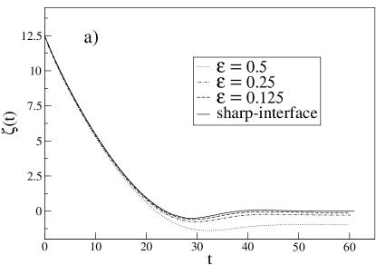
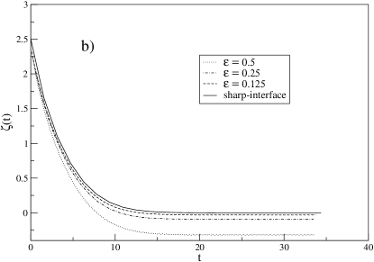
Figure 1: Evolution of the interface position during the transient for (a) $l_{T}/l=12.5$ and (b) $l_{T}/l=2.5$, and convergence to the sharp-interface as $\varepsilon\rightarrow 0$.

We now estimate the transient dispersion relation $\omega(kl,t)$ from PFM simulations and compare it with the sharp interface prediction of Eqs. (70, 71). To this end we simulate for each desired value of $t$ a (planar) 1D interface evolving from $t_{0}=0$ to $t$. At that moment we introduce a sinusoidal interface perturbation with wavevector $kl$, and continue the simulation in 2D. The spectral analysis of the front allows us to locate the regime where the mode evolution is linear. This is represented in Fig. 2a, where three definite regions can be observed. From the linear region the value of the transient growth rate $\omega(kl,t)$ is calculated. Fig. 2b shows the growth rate at different times obtained for two different modes $kl=1.25$ and $kl=2.5$ in the case of $l_{T}/l=12.5$ and $d_{0}/l=0.06923$. Quantitative agreement is observed for all times.

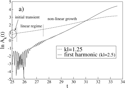
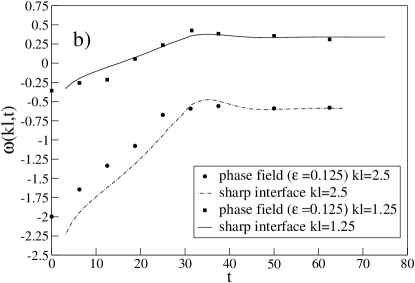
Figure 2: a) Localization of the linear growth regime of the mode $kl=1.25$. b) Time evolution of two different modes $kl=1.25$ and $kl=2.5$ for $l_{T}/l=12.5$.

We can now introduce internal fluctuations in the diffusion equation of the phase-field by introducing the noises appearing in Eqs. (10-13). In simulations the growth of a range of wavelengths can be observed until a selected mode dominates. The spectral analysis of the front reveals quantitative agreement during the linear regime between the growth of each mode and the transient dispersion relation predicted by the sharp interface model. In Fig. 3 we present the amplitude of one of the modes ($kl=2.5$, $l_{T}/l=12.5$) averaged for 15 different noise realizations. There is a good agreement in the regime with positive $\omega$ (i.e. were an increasing $A_{k}(t)$ is predicted).

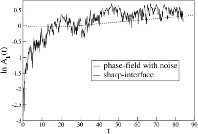
Figure 3: Time evolution of the mode $kl=2.5$ ($l_{T}/l=12.5$) with the phase-field with noise, and comparison with the sharp-interface prediction.

4.2 Dendritic sidebranching in free solidification

In the previous Section our interest was the initial destabilization of the planar interface in solidification experiments, and the influence of the internal noise. That transient has relevance in the selection of the wavelength of the dendritic array. In the present Section our interest will lie in some characteristics of the dendrite itself, in particular in those of the sidebranching. We study the noise–induced sidebranching scenario in the linear regime and in particular we focus on the issue of the internal vs. external origin of the noise [38].

In a frame of reference moving with the tip of the dendrite, sidebranching can be seen as a wave that propagates along the dendrite away from the tip at the tip’s velocity. Therefore, an appropriate characterization is provided by the amplitude of the wave. Brener and Temkin [105] pointed out that experimentally observed sidebranching could be explained by considering noise of thermal origin. They analytically found that the growth of sidebranching amplitude in the linear regime behaves exponentially as a function of $z^{2/5}$. Dougherty et al. [110] studied sidebranching in experiments with ammonium bromide dendrites. The sidebranching amplitude was found to increase exponentially up to a certain value of $z$, from which the linear theory is presumably no longer valid. It was also observed that side branches separated by more than about six times the mean wavelength are uncorrelated.

Bisang and Bilgram [111] found a quantitative agreement between the predictions for the linear regime in Ref. [105] and their results in experiments with xenon dendrites. They concluded that Brener and Temkin calculations describe correctly the sidebranching behaviour of dendrites for any pure substance with cubic symmetry and thus thermal noise was the origin of the sidebranching observed in their experiments.

Karma and Rappel [39] included thermal noise in a two–dimensional PFM for solidification controlled by heat diffusion, and obtained a good quantitative agreement between the computed sidebranching amplitude and wavelength as a function of distance to the tip and the predictions of the linear $WKB$ theory for anisotropic crystals in two dimensions. For a needle crystal shape $x\sim z^{3/5}$, sidebranching amplitude was found to increase exponentially as a function of $z^{2/5}$.

However, the extension of the theory of dendritic sidebranching to the growth controlled by solutal diffusion shows that there are indications that in some experiments internal thermodynamical fluctuations could not account for the observed sidebranching activity [38]. In that case, some other source of fluctuations, of external origin, should be invoked. We study some of the consequences derived from adding a non–conserved noise source into a two–dimensional PFM. This noise is of very different nature than what one should employ to account for internal fluctuations.

4.2.1 Sidebranching characteristics

We have performed simulations of dendritic growth by employing a PFM for solidification with anisotropy included in the surface tension [20], which has been taken as $\sigma=\sigma(0)(1+\gamma_{su}cos(4\theta))$. Whereas internal fluctuations would have appeared as a stochastic current (and, therefore, as a conserved term) in the equation for the diffusion field and an additional stochastic term in the phase field equation , like in Eqs. (8,9), we have chosen to model an external source of fluctuations by a non–conserved random term added to the equation for $u$. This random term reads simply $I\cdot r$, where $I$ denotes the amplitude of the noise, and $r$ is a uniform random number in the interval $[-0.5,0.5]$. More details about the employed numerical procedure and the selection of parameters can be found in Ref. [38].

A growing dendrite obtained by means of the PFM is shown in Fig. 4. Side branches appear at both sides of the main dendrite, yielding approximately a $90^{o}$ angle with it, like it was observed in Ref. [110]. Far down the tip one can clearly observe competition between branches which gives rise to a coarsening effect.

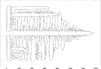
Figure 4: Dendrite obtained with the PFM with an external noise term.

In order to study the sidebranching induced by noise we have measured the half–width $h_{z}(t)$ of the dendrite at various distances $z$ behind the tip as a function of time. The half–width of the dendrite as a function of time and its power spectrum $P_{z}(f)$ are shown in Fig. 5 for a distance $z=100$ grid points. The data used to compute the power spectrums were six times the shown lengths. We also computed the cross–correlation function

$$C(t^{\prime})=<[h_{Lz}(t+t^{\prime})-\bar{h}_{Lz}][h_{Rz}(t)-\bar{h}_{Rz}]>/\sigma_{L}\sigma_{R},$$ (74)

where $h_{Lz}(t)$, $h_{Rz}(t)$, $\sigma_{L}$ and $\sigma_{R}$ are the half–width functions and their standard deviations for the two sides of the dendrite at the same distance from the tip. We found that $C(0)$ is around $0.4$ for points very close to the tip and that its value decreases very quickly to $0$ when increasing $z$. The same behavior was observed in the experiments in Ref. [110].

In Fig. 6 we show the logarithm of the square root of the area under the spectral peak as a function of $z$. This representation gives the behavior of the amplitude of the sidebranching as a function of the distance to the tip. The amplitude has a different behavior for $z$ up to $100$ (linear regime) and for values greater than this one (nonlinear regime). In the region near the tip the amplitude increases exponentially with $z^{2/5}$, while far down from the tip the growth rate of the amplitude is slower. Thus, the behavior of the data obtained in the simulations is consistent with the linear analysis carried out in Refs. [39, 105] up to a certain value of $z$.

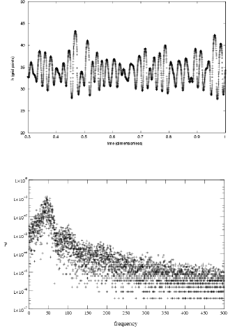
Figure 5: Half–width $h_{z}(t)$ of the dendrite (up) and its power spectrum $P_{z}(f)$ (down) for $z=100$.

Figure 6: Square root of the area under the spectral peak as a function of $z$.

In conclusion, despite thermal noise could not always be the main origin of sidebranching, its qualitative characteristics are common for noise-induced sidebranching independently of its origin.

4.3 Mesophase transitions in liquid crystals

The growth of liquid crystal interfaces in transitions between mesophases is in many aspects analogous to that of solidification interfaces. The basic description is expected to be the same, lying the main differences in the parameter ranges, which often makes the liquid crystal case particularly suitable from an experimental point of view. From a theoretical point of view, a significant parameter difference with respect to the solidification case is the one associated to the diffusion coefficients, which are of the same order of magnitude in the two liquid crystal phases. Another distinct feature is the presence of strong anisotropies, both at the interface, which can be faceted, and in the transport properties in the bulk. In this Section we will show how these anisotropies, introduced into a PFM, can account for the morphologies obtained in different growth conditions.

4.3.1 Anisotropic surface tension

We have considered a liquid crystalline substance, CCH3, which presents a N–SmB phase transition at temperature $T_{NS}$. The pattern formation during the N-SmB phase transition can be observed experimentally in a quasi two–dimensional geometry [29, 30]. The sample was initially set above the phase transition temperature $T_{NS}$, and was suddenly undercooled below this temperature in such a way that small smectic–B germs nucleated and started to grow.

From the equilibrium shape one can obtain the corresponding angular dependence of the normalized surface tension $\eta(\theta)={\sigma(\theta)\over\sigma(0)}$ (being $\theta=0$ the direction parallel to the smectic layers) by means of the Wulff–construction [112]. The function for CCH3 is [29, 30]: $\eta(\theta)=1.00-0.35\theta^{2}+0.01\theta^{4}$ in the range $|\theta|\leq\pi/2$, while $\eta(\theta)=\eta(\pi-\theta)$. Clearly $\eta(\theta)$ has cusps at $\theta=\pm\pi/2$.

Out of equilibrium, CCH3 presents three different morphologies, ranging from a slightly deformation of the equilibrium shape, to a butterfly-like morphology and, finally in the largest undercooling regime, to a four-fold dendritic shape [29, 30, 32].

The nematic – smectic–B (N–SmB) phase transition is of first order, therefore standard models for solidification can be applied. Like in the previous section, we have employed the anisotropic PFM of Ref. [20]. In simulations the kinetic term was taken isotropic. The employed numerical procedure was described in [29]. We have simulated one quarter of the full experimental system by locating the initial smectic–B seed in the lower left corner. Symmetrical (reflecting) boundary conditions for $\phi$ and $u$ have been imposed on the four sides of the system.

The four main morphologies of CCH3 have been computationally reproduced on a qualitative level. At small dimensionless undercooling, simulations show a very slow growth of the germ, which at the observed times maintains a rectangle–like shape very similar to the equilibrium one in experiments, i.e., with two parallel facets and two rough convex sides (Fig. 7). The growth velocity of the facets is smaller than that of the convex parts of the interface.

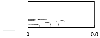
Figure 7: CCH3. N–SmB interface (points with $\phi=0.5$) obtained from simulation at subsequent times. $\Delta=0.05$.

At slightly larger undercoolings, the short sides undergo a first instability from convex to concave (Fig. 8).

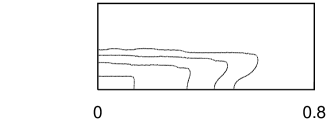
Figure 8: CCH3. N–SmB interfaces ($\phi=0.5$) obtained from simulation at subsequent times. $\Delta=0.09$.

At larger values of the undercooling the faceted sides start to bend adopting a slightly concave curvature and macroscopic facets disappear with the four corners opened up, forming a butterfly–like shape (Fig. 9).

Figure 9: CCH3. N–SmB interfaces ($\phi=0.5$) obtained from simulation at subsequent times. $\Delta=0.2$.

Finally, a completely developed four-fold dendrite is obtained in the large undercooling regime (Fig. 10).

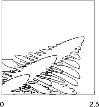
Figure 10: CCH3. N–SmB interface ($\phi=0.5$) obtained from simulation at subsequent times. $\Delta=0.7$.

4.3.2 Anisotropic heat diffusion

It has been proved in the previous Section the important role played by the surface tension anisotropy in the selection of the steady–state shape of a growing interface. Aside from this one and kinetic anisotropy, systems such as liquid crystals do present considerable anisotropies in their transport coefficients [113, 114, 115, 116] and their effects are potentially significant in interfacial growth phenomena. We address here the growth of dendrites subject to anisotropy in the heat diffusion coefficient, and its consequences on the growth morphologies [33].

When the anisotropic thermal diffusion is implemented in a PFM, the $\phi$–equation does not change and the $u$–equation should be slightly modified to consider a diffusion matrix $D_{ij}$. The numerical details can be found in Refs. [33, 32].

The experimental system used to study the thermal diffusion anisotropy is the liquid crystalline substance CCH4, and in particular its N–SmB phase transition. At large undercoolings, some SmB seeds whose director directions do not match that of the sorrounding N phase, present a non-reflection symmetry in their growth.

With the modified PFM, it is possible to reproduce such experimental morphologies. This is observed in the numerical simulation (Fig. 11). Although the used set of parameters could differ from those real material ones, the qualitative resemblance with experimental results is remarkably good [33]. Axis $x,y$ has been placed along the principal directions of the diffusion matrix, in order to have only diagonal terms in the equation. Anisotropy in the diffusion, defined as $(D_{max}-D_{min})/D_{min}$, has taken a value of $0.5$, very similar to experimental estimates. The surface free energy has been rotated in the $(x,y)$ plane, accounting for different orientations of the director in each phase.

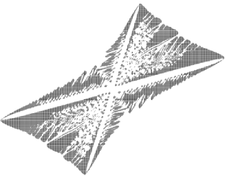
Figure 11: Simulation for the non–reflection symmetry.

It can be derived from Fig. 11 that the reflection symmetry has been broken by the inclusion of the anisotropic heat diffusion (previous simulations with rotated surface tension function and isotropic heat diffusion did not show the asymmetry in the growth velocities). In both experiments and simulations the most developed branches are systematically those growing in the direction of lowest heat diffusion. Therefore one can conclude that heat diffusion anisotropy favours dendritic growth in the lowest diffusion directions. This means that the relevant heat diffusion process is the one that occurs in the direction perpendicular to the axis of the dendrite.

4.4 Results on Viscous Fingering

The purpose of the present Section is to illustrate the practical use of the PFM in the case of viscous fingering, with direct quantitative tests of the thin-interface approximation to assess the usefulness of the approach in this case. Indeed, the fact that the model has the correct sharp-interface limit does not guarantee its practical usefulness for several reasons. On the one hand, the stability of both the bulk phases and the kink profile must be assured, since this might not be the case in general. On the other hand, a direct empirical test is necessary to determine quantitatively how close a finite $\epsilon$ situation is to the sharp-interface limit. This means finding a set of explicit quantitative criteria to choose all the nonphysical parameters in order to ensure a desired accuracy. Finally, it is interesting to find to what extent that model can provide quantitative results with reasonable computing efforts in actual simulations.

4.4.1 Linear dispersion relation

The first situation in which the model can be tested is the linear regime of a perturbed planar interface. The linear dispersion relation has been computed for vanishing viscosity contrast ($c=0$). The sharp-interface model predicts a linear growth that does not depend on $c$. However, the phase field model should exhibit some dependence in the viscosity contrast related to the finite-$\epsilon$ and -$\tilde{\epsilon}$ corrections (see Sec. IV in Ref. [43]).

We use a single mode occupying the whole channel width (i.e., of wavelength 1 and wavevector $k=2\pi$) and then vary the dimensonless surface tension $B$ in order to change the growth rate of that mode according to the Hele–Shaw dispersion relation

$$\omega_{0}=|k|(1-Bk^{2}).$$ (75)

This is physically completely equivalent to fixing the surface tension and varying the wavevector of the mode, as can be seen through the rescaling $k^{\prime}=\sqrt{B}k,\omega^{\prime}_{0}=\sqrt{B}\omega_{0}=|k^{\prime}|(1-k^{\prime 2})$. However, it is numerically more convenient, since it allows one to use the same value of $\epsilon$ for all the modes, because $k$ is fixed. Thus, according to the finite-$\epsilon$ and -$\tilde{\epsilon}$ dispersion relation derived in Sec. IV of Ref. [43],

$$\omega=\omega_{0}(\frac{1}{\sqrt{1+\frac{\tilde{\epsilon}\omega}{k^{2}}}}-\epsilon|k|{\sqrt{2}}\frac{5}{6})+{\cal O}(c^{2})+{\cal O}(\epsilon^{2}).$$ (76)

We have used $\epsilon=0.01$, $\tilde{\epsilon}=0.1$ for the deviation from the sharp-interface one, $\omega_{0}$, to keep below a 10%.

Figure 12: Linear dispersion relation in scaled variables

In Fig. 12 we present the linear dispersion relation thus obtained in scaled variables. The points (+) correspond to the measured growth rates for roughly a decade in the amplitude. Their deviation from the sharp-interface result of Eq. (75) (solid line) keeps below the desired 10% error and is fairly well quantitatively predicted by the thin-interface dispersion relation of Eq. (76) (dotted line). This quantitative agreement between theory and numerics is quite remarkable if we take into account that the thin-interface model is based on an asymptotic expansion in $\epsilon$. This good agreement is indeed an indication that the value of $\epsilon$ used is in the asymptotic regime of the sharp-interface limit, as we will see more clearly in Fig. 13.

Figure 13: Convergence to the Hele-Shaw value for the maximum of the linear dispersion relation curve

The growth rate values shown in Fig. 12 could still be refined by further decreasing $\epsilon$ and $\tilde{\epsilon}$. This is not only a theoretical possibility, but can also be done in practice as we show in Fig. 13, although the computation time increases as explained above. Here, we study the convergence of the growth rate $\omega$ (y-axis) for the maximum of $\omega^{\prime}(k^{\prime})$ ($B=8.443...\times 10^{-3}$) to the Hele–Shaw result $\omega_{0}=4.188...$ (left upper corner) as we decrease $\epsilon$ (x-axis) and $\tilde{\epsilon}$ (various symbols). The empty symbols have been obtained with $\Delta x=\epsilon$, whereas the filled ones correspond to $\Delta x=\epsilon/2$. The growth rates obtained with $\Delta x=\epsilon$ are always below the ones for $\Delta x=\epsilon/2$, probably because of the stabilizing effect of the mesh size. If $\Delta x$ is further decreased the differences with the values computed with $\Delta x=\epsilon/2$ are tiny, whereas the gap between the $\Delta x=\epsilon$ and the $\Delta x=\epsilon/2$ points is pretty large (clearly more than the differences between distinct symbols —distinct $\tilde{\epsilon}$ values— or adjacent values of $\epsilon$). This means that the discretization has practically converged to the continuum model for $\Delta x=\epsilon/2$, but not for $\Delta x=\epsilon$. That is the reason why we have used $\Delta x=\epsilon/2$ in Fig. 12.

Moreover, the $\Delta x=\epsilon/2$ points should be described by the thin-interface model of Eq. (76), and this is indeed the case for small enough values of $\epsilon$. To visualize this we have plotted the thin-interface prediction for $\tilde{\epsilon}=0$ (dashed line), which is, of course, a straight line in $\epsilon$. Each set of points with a same $\tilde{\epsilon}$ value clearly tends to align parallel to this line as $\epsilon$ decreases —as Eq. (76) predicts—, whereas they curve up and even cross the line for large values of $\epsilon$, for which we are beyond the asymptotic regime of validity of Eq. (76), apparently ending near $\epsilon=0.01$. This makes $\epsilon=0.01$ very suitable for simulations, and confirms it to be within the asymptotic regime as we pointed out above. Note as well how the growth rate increases with decreasing values of $\tilde{\epsilon}$ within the same value of $\epsilon$ (vertical columns of points), and how it approaches the dashed line in good agreement with the values predicted by Eq. (76) for values of $\epsilon$ within the asymptotic regime.

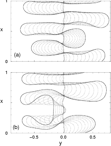
Figure 14: Time evolution of the interface a) $c=0$ b) $c=.8$

4.4.2 Finger dynamics

The quantitative test in the nonlinear regime are not so simple due to the lack of exact analytical solutions. For the case of asymptotic Saffman–Taylor fingers, for instance, only partial numerical information is available, in particular for varying viscosity contrast. A detailed comparison with existing evidence was carried out in Ref. [44]

At a qualitative level, however, it is illustrative to plot an example of multifinger dynamics, in particular to emphasize the importance to have the viscosity contrast as an explicit parameter in the model. Indeed, the scenario of finger competition in the high viscosity contrast limit, where larger fingers screen out the smaller ones, is actually valid only for $c$ very close to $1$. In contrast, the persistence of the small fingers, which is characteristic of low viscosity contrasts, seems to be the generic case [101].

Here we use a somewhat experimentally realistic initial condition consisting of a superposition of sinusoidal modes with random, uniformly distributed amplitudes between -0.005 and +0.005 for each wavelength $\lambda=1,\frac{1}{2},\frac{1}{3}...\frac{1}{7}$ —i.e., in the linear regime and random phases. For $B=10^{-3}$ the most amplified of these wavelengths will be $\lambda=\frac{1}{3}$, so that we expect 3 unequal fingers to appear and there is a chance for mode interaction and competition to set in. Wavelengths below $\lambda=0.161...$ are stable and will decay. We include some of them anyway. Then all modes are added up to find the interface position. The stream function predicted by the linear theory is also obtained by adding up the stream function of each mode, but all with their peaks centered at the same final interface position, to avoid the formation of more than one peak of the stream function across the interface.

Since harmonics of the channel width are present, we have to refine the $\epsilon$ used in the linear regime. We use $\epsilon=0.00625$, with $\Delta x=\epsilon$ to save computation time. The value of $\tilde{\epsilon}$ is quite crude ($\tilde{\epsilon}=0.5$) for the equal viscosities case $c=0$, Fig. 14a, and especially for the high viscosity contrast ($c=0.8$) run Fig. 14b ($\tilde{\epsilon}=0.2$).

The results are shown in Figs. 14a,b for $0.15<t<1.25$ at constant time intervals 0.1 (dots). The last interface is emphasized in bigger points (+) and the solid line corresponds to the initial condition for $t=0$. As we can see, the initial condition happens to have six maxima. Rather quickly, only three of them are left out as predicted by linear stability, even before entering the non-linear regime, in which these maxima elongate into well developed fingers. For vanishing viscosity contrast ($c=0$, Fig. 14a), there is no apparent competition, in agreement with experimental [100] and numerical [90, 95, 101] evidence. Longer and shorter fingers all advance. Shorter fingers might not advance so quickly, but they expand to the sides, so they clearly keep growing. In contrast, starting with the same initial condition that for $c=0$, the $c=0.8$ run (Fig. 14b) shows competition between fingers of the less viscous fluid advancing into the more viscous one, as it is known to happen in the Saffman–Taylor problem. The shorter finger now also expands laterally, but it soon begins to move backwards as a whole. Longer times may lead to the pinch-off of droplets in both cases [101].

In summary the basic criteria to control the closeness to the sharp interface limit are $\epsilon\kappa<<1$, $\frac{\tilde{\epsilon}\omega}{(1\pm c)k^{2}}<<1$. More precisely, we find numerically that the thin-interface model is accurate in the linear regime with an error below below 10% if one satisfies the conditions $\epsilon k\leq 0.06$, $\frac{\tilde{\epsilon\omega}}{(1\pm c)k^{2}}\leq 0.016$. The method could be made more efficient by using an adaptive mesh or (possibly) by cancelling out the corrections to the sharp-interface equations remaining (i.e., other than the Allen–Cahn law) in the thin-interface model. For high viscosity contrasts, $c\sim 1$, a distinct model could possibly be more efficient. From the recent progress in boundary-integral methods [98], however, the use of PFM may not be significantly advantageous in this problem except maybe for the natural incorporation of interface pinch-off. Nevertheless, the application of the PFM approach in three-dimensional viscous flows in porous media, is yet an unexplored and promising future direction.

5 Conclusions

Phase-field modeling of interface dynamics in nonequilibrium systems has proved to be a very useful tool. In this chapter we have reviewed different aspects of this active field of research. Phase-field models introduce an auxiliary field to allow for a diffuse interface. This additional field is coupled to the physical fields in such a way that the macroscopic, sharp-interface boundary conditions are effectively reproduced. In this way, a free-boundary problem is transformed into a set of partial differential equations, usually much simpler to handle. In this chapter a phase-field model for solidification has been explicitly derived from a free energy. As a second example, a phase-field model for the Saffman–Taylor problem has been presented. In this case the derivation is not based on a free-energy functional. The thin-interface approximation, which includes corrections on the interface thickness, have been discussed for these two examples. We have also presented some illustrative applications such as the study of fluctuations in directional solidification of alloys and dendritic sidebranching in free solidification, growth of mesophases in liquid crystals and the dynamics of viscous fingering.

At the present level of development of phase-field model techniques, these have been shown to be quantitatively accurate with reasonable computational cost, and usually advantageous with respect to other techniques in different aspects. Phase-field models are simple to be implemented in a computer and contain a complete description of the full nonlinear and nonlocal properties of the macroscopic free-boundary problems. In addition, in the phase-field framework it is relatively simple to introduce additional perturbations, such as fluctuations and static disorder, or modifications of the boundary conditions. Future lines of research will certainly include quantitative studies of interfaces in three dimensions, the consideration of complex fluids and biological systems, and possibly applications at the nanoscale. Undoubtly the phase-field approach holds the promise of fruitful applications to new problems in years to come.

References

- [1] B.I. Halperin, P.C. Hohenberg and S.–K. Ma, Phys. Rev. B 10, 139 (1974); P.C. Hohenberg and B.I. Halperin, Rev. Mod. Phys. 49, 435 (1977).
- [2] G.J. Fix, in Free Boundary Problems: Theory and Applications, Ed. A. Fasano and M. Primicerio, p. 580, Pitman (Boston, 1983).
- [3] J.S. Langer, Models of pattern formation in first–order phase transitions, in Directions in Condensed Matter Physics p. 165, Ed. G. Grinstein and G. Mazenko, World Scientific, Singapore, (1986).
- [4] J.B. Collins and H. Levine, Phys. Rev. B 31, 6119 (1985).
- [5] G. Caginalp, in Applications of Field Theory to Statistical Mechanics, Ed. L. Garrido, Lecture Notes in Physics, Vol. 216, p. 216, Spinger–Verlag (Berlin, 1985); G. Caginalp and P. Fife, Phys. Rev. B 33, 7792, (1986); G. Caginalp, Arch. Rat. Mech. Anal. 92, 205 (1986); in Material Instabilities in Continuum Problems and Related Mathematical Problems, p.35, Ed. J.M. Ball, Oxford University Press, (Oxford, 1988); G. Caginalp and P.C. Fife, SIAM J. Appl. Math., 48, 506, (1988); G. Caginalp and X. Chen, in On the Evolution of Phase Boundaries, Vol. 43 of The IMA Volumes in Mathematics and Its Applications, p. 1, Ed. M.E. Gurtin and G.B. McFadden, Springer–Verlag, (New York, 1992).
- [6] G. Caginalp, Ann. of Phys., 172, 136 (1986).
- [7] G. Caginalp, Phys. Rev. A, 39, 5887 (1989).
- [8] G. Caginalp and E.A. Socolovsky, J. Comput. Phys. 95, 85 (1991).
- [9] M.E. Gurtin, in Metastability and Incompletely Posed Problems, Vol. 3 of The IMA Volumes in Mathematics and Its Applications, p. 135, Ed. S. Antman and J.L. Ericksen and D. Kinderlehrer and I. Muller, Springer–Verlag (New York, 1987).
- [10] P.C. Fife and G.S. Gill, Phys. D 35, 267 (1989); Phys. Rev. A 43, 843 (1991).
- [11] G. Caginalp and P. Fife, Phys. Rev. B 34, 4940 (1986); G. Caginalp and J.–T. Lin, IMA J. Appl. Math. 39, 51 (1987).
- [12] G. Caginalp, IMA J. Appl. Math. 44, 77 (1990).
- [13] G. Caginalp, Rocky Mtn. J. Math. 21, 603 (1991).
- [14] O. Penrose and P.C Fife, Physica D 43, 44 (1990); 69, 107 (1993).
- [15] J.B. Smith, J. Comput. Phys. 39, 112 (1981); A.R. Umantsev and V.V. Vinograd and V.T. Borisov, Sov. Phys. Crystallogr. 30, 262 (1986); 31, 596 (1986); J.–T. Lin, The Numerical Analysis of a Phase Field Model in Moving Boundary Problems, PhD Thesis, Carnegie Mellon University (1984); S.A. Schofield and D.W. Oxtoby, J. Chem. Phys. 94, 2176 (1991); H. Löwen and J. Bechhoefer and L. Tuckerman, Phys. Rev. A 45, 2399 (1992).
- [16] R. Kobayashi, Physica D 63, 410 (1993).
- [17] R. Kobayashi, Exper. Math. 3, 59 (1994).
- [18] A.A. Wheeler and W.J. Boettinger and G.B. McFadden, Phys. Rev. A 45, 7424 (1992).
- [19] A.A. Wheeler, W.J. Boettinger and G.B. McFadden, Phys. Rev. E 47, 1893 (1993).
- [20] S–L. Wang, R.F. Sekerka, A.A. Wheeler, B.T. Murray, S.R. Coriell, R.J. Braun and G.B. McFadden, Physica D 69, 189 (1993).
- [21] G.B. McFadden, A.A. Wheeler, R.J. Braun, S.R. Coriell and R.F. Sekerka Phys. Rev. E 48, 2016 (1993).
- [22] R.J. Braun, G.B. McFadden and S.R. Coriell, Phys. Rev. E 49, 4336 (1994).
- [23] R. Kupferman, O. Shochet, E. Ben–Jacob and Z. Schuss, Phys. Rev. B 46, 16045 (1992).
- [24] J.A. Warren and W.J. Boettinger, Acta Metall. 43, 689 (1995).
- [25] A.A. Wheeler and B.T. Murray and R.J. Schaefer, Physica D 66, 243 (1993).
- [26] S–L. Wang and R.F. Sekerka, Phys. Rev. E 53, 3760 (1996).
- [27] B.T. Murray, A.A. Wheeler and M.E. Glicksman, J. Cryst. Growth 154, 386 (1995).
- [28] F. Marinozzi, M. Conti and U. Marini Bettolo Marconi, Phys. Rev. E 53, 5039 (1996).
- [29] R. González–Cinca, L. Ramírez–Piscina, J. Casademunt, A. Hernández–Machado, L. Kramer, T. Tóth Katona, T. Börzsönyi and Á. Buka, Physica D 99, 359 (1996).
- [30] T. Tóth Katona, T. Börzsönyi, Z. Váradi, J. Szabon, Á. Buka, R. González–Cinca, L. Ramírez–Piscina, J. Casademunt and A. Hernández–Machado, Phys. Rev. E 54, 1574 (1996).
- [31] Gamil Aly Shalaby, The Growth of a Liquid Crystal, PhD Thesis, Institute of Physics, University of Bayreuth (1996).
- [32] R. González-Cinca, A Phase-field Model Study of Pattern Formation in Crystal Growth, PhD Thesis, Department of Applied Physics, Technical University of Catalonia (2000).
- [33] R. González-Cinca, L. Ramírez-Piscina, J. Casademunt, A. Hernández-Machado, T. Tóth Katona, T. Börzsönyi and Á. Buka, J. Cryst. Growth 193, 712 (1998).
- [34] T. Börzsönyi and Á. Buka and L. Kramer, Phys. Rev. E 58, 6236 (1998).
- [35] R. Kupferman, O. Shochet and E. Ben–Jacob, Phys. Rev. E 50, 1005 (1994).
- [36] J.L. Mozos and H. Guo, Europhys. Lett. 32, 61 (1995).
- [37] P.W. Bates and P.C. Fife and R.A. Gardner and C.K.R.T. Jones, Physica D 104, 1 (1997).
- [38] R. González-Cinca, L. Ramírez-Piscina, J. Casademunt, and A. Hernández- Machado, Phys. Rev. E 63 051602 (2001).
- [39] A. Karma and W–J. Rappel, Phys. Rev. E 60, 3614 (1999).
- [40] S.G. Pavlik and R.F. Sekerka, Physica A 268, 283 (1999); Physica A 277 415 (2000).
- [41] R. F. Almgren, SIAM J. Appl. Math. 59, 2086 (1999).
- [42] M. Ben Amar, Phys. Fluids A, 4, 2641 (1992).
- [43] R. Folch, J. Casademunt, A. Hernández-Machado and L. Ramírez-Piscina, Phys. Rev. E 60, 1724 (1999).
- [44] R. Folch, J. Casademunt, A. Hernández-Machado and L. Ramírez-Piscina, Phys. Rev. E 60, 1734 (1999).
- [45] T. Biben and C. Misbah, Eur. Phys. J. B 29, 311 (2002); Phys. Rev. E 67, 031908 (2003).
- [46] A. Karma and W–J. Rappel, Phys. Rev. E 53, R3017 (1996); Phys. Rev. Lett. 77, 4050 (1996).
- [47] A. Karma and W–J. Rappel, Phys. Rev. E 57, 4323 (1998).
- [48] A. Karma, Phys. Rev. Lett. 87, 115701 (2001).
- [49] R. Folch, A. Karma and M. Plapp (in preparation).
- [50] R. Folch and M. Plapp, cond-mat/0303449 (2003).
- [51] K. R. Elder, M. Grant, N. Provatas and J.M. Kosterlitz, Phys. Rev. E 64, 021604 (2001).
- [52] R.J. Braun and B.T. Murray, J. Cryst. Growth 174, 41, (1997); N. Provatas and N. Goldenfeld and J. Dantzig, Phys. Rev. Lett. 80, 3308, (1998); J. Comp. Phys. 148, 265 (1999).
- [53] M. Plapp and A. Karma, Phys. Rev. Lett. 84, 1740 (2000); J. Comp. Phys. 165, 592 (2000).
- [54] A. Karma, Y. H. Lee, and M. Plapp, Phys. Rev. E 61, 3996 (2000); J. Bragard, A. Karma, Y. H. Lee, and M. Plapp, Interface Science 10, 121 (2002).
- [55] A. Bösch, H. Müller–Krumbhaar and O. Shochet, Z. Phys. B 97, 367, (1995).
- [56] R. Tönhardt and G. Amberg, J. Cryst. Growth 194, 406 (1998); H. J. Diepers, C. Beckermann and I. Steinbach, Acta Mater., 47, 3663 (1999); C. Beckermann, H. J. Diepers, I. Steinbach, A. Karma and X. Tong, J. Comp. Phys., 154, 468 (1999); 213, 161 (2000). X. Tong, C. Beckermann and A. Karma, Phys. Rev. E 61, R49 (2000); X. Tong, C. Beckermann, A. Karma and Q. Li, Phys. Rev. E 63, 061601 (2001); D.M. Anderson, G.B. McFadden and A.A. Wheeler Physica D 135, 175 (2000); 151 (2-4): 305 (2001).
- [57] J.-H. Jeong, N. Goldenfeld and J. Dantzig, Phys. Rev. E 64, 041602 (2001).
- [58] R. Tönhardt and G. Amberg, Phys. Rev. E 62, 828 (2000).
- [59] D. Jacqmin, J. Comput. Phys. 155, 96 (1999).
- [60] K.R. Elder, F. Drolet, J.M. Kosterlitz and M. Grant, Phys. Rev. Lett. 72, 677 (1994); A. Karma, Phys. Rev. E 49, 2245 (1994).
- [61] A.A. Wheeler, G.B. McFadden and W.J. Boettinger, Proc. R. Soc. London, Ser. A 452, 495, (1996).
- [62] T. S. Lo, A. Karma, and M. Plapp, Phys. Rev. E 63, 031504 (2001).
- [63] I. Steinbach et al., Physica D 94, 135 (1996).
- [64] H. Garcke, B. Nestler, and B. Stoth, SIAM J. Appl. Math. 60, 295 (1999).
- [65] R. Folch and M. Plapp, cond-mat/0206237 (2002).
- [66] W. J. Boettinger, J. A. Warren, C. Beckermann and A. Karma, Annu. Rev. Mater. Res. 32, 163 (2002).
- [67] M. Conti, Phys. Rev. E 55, 701 (1997); Phys. Rev. E 55, 765 (1997).
- [68] A. Roy and J.M. Rickman and J.D. Gunton and K.R. Elder, Phys. Rev. E 57, 2610 (1998).
- [69] R. Kobayashi, J.A. Warren and W.C. Carter, Physica D, 140, 141 (2000); A.E. Lobkovsky and J.A. Warren, Physica D, 164, 202 (2002).
- [70] R. Kam and H. Levine, Phys. Rev. E 52, 4553 (1995); Phys. Rev. E 54, 2797 (1996); A. Karma and M. Plapp, Phys. Rev. Lett. 81, 4444 (1998).
- [71] J. Müller and M. Grant, Phys. Rev. Lett. 82, 1736 (1999); K. Kassner, C. Misbah, J. Müller, J. Kappey and P. Kohlert, Phys. Rev. E 63, 036117 (2001).
- [72] D. Rodney, A. Finel, MRS Symposium Proc. 652, Y4.9.1 (2001); D. Rodney, Y. Le Bouar, A. Finel, Acta Mater. 51, 17 (2003); Y. U. Wang, Y. M. Jin, A. M. Cuitino and A. G. Khachaturyan, Acta Mater. 49, 1847 (2001); Appl. Phys. Lett. 78, 2324 (2001); S.Y. Hu, L.Q. Chen, Acta Mater. 49, 463 (2001).
- [73] A. Karma, D. Kessler and H. Levine, Phys. Rev. Lett. 87, 045501 (2001).
- [74] L.-Q. Chen, Annu. Rev. Mater. Res. 32, 113 (2002).
- [75] Hyeong-Gi Lee, J. S. Lowengrub and J. Goodman, Phys. Fluids 14, 492 (2002); 14, 514 (2002)
- [76] See, e. g. U. Ebert and W. van Saarloos, Phys. Rep. 337, 139 (2000).
- [77] J. Müller and W. van Saarloos, Phys. Rev. E 65, 061111 (2002).
- [78] A. Hernández-Machado, A.M. Lacasta, E. Mayoral and E. Corvera Poiré, A phase-field model of Hele-Shaw flows in the high viscosity contrast regime, Preprint (2003).
- [79] M. Castro, cond-mat/0212524 (2003).
- [80] M. Dubé, M. Rost, K.R. Elder, M. Alava, S. Majaniemi and Ala-Nissila, Phys. Rev. Lett. 83, 1628 (1999); Eur. Phys. J. B, 15 701 (2000).
- [81] A. Hernández-Machado, J. Soriano, A.M. Lacasta, M.A. Rodríguez, L. Ramírez-Piscina and J. Ortín, Europhys. Lett. 55, 194 (2001).
- [82] J.S. Langer, Rev. Mod. Phys. 52, 1 (1980).
- [83] R. Benítez, and L. Ramírez-Piscina (in preparation).
- [84] D.A. Kessler, J. Koplik and H. Levine, Adv. Phys., 35, 255 (1988); P. Pelcé, Dynamics of Curved Fronts. Persp. in Physics, Academic Press (1988).
- [85] P.G. Saffman and G.I. Taylor, Proc. R. Soc. London A, 245, 312 (1958);
- [86] D. Bensimon, L. Kadanoff, S. Liang, B.I. Shraiman and C. Tang, Rev. Mod. Phys., 58, 977 (1986).
- [87] K.V. McCloud and J.V. Maher, Phys. Rep. 260, 139 (1995)
- [88] Y. Couder, Viscous fingering as an archetype for growth patterns in Perspectives in Fluid Dynamics, Cambridge University Press (2000);
- [89] S. Tanveer, Surprises in viscous fingering, J. Fluid Mech., 409, 273 (2000).
- [90] G. Tryggvason and H. Aref, J. Fluid Mech., 136, 1-30 (1983); J. Fluid Mech., 154, 287-301 (1985).
- [91] M. Siegel and S. Tanveer, Phys. Rev. Lett. 76, 419 (1996); F.X. Magdaleno and J. Casademunt, Phys. Rev. E 57, R3707 (1998).
- [92] J. Casademunt and F.X. Magdaleno, Phys. Rep. 337, 1 (2000).
- [93] E. Pauné, F.X. Magdaleno and J. Casademunt, Phys. Rev. E 65, 056213 (2002); E. Pauné, M. Siegel and J. Casademunt, Phys. Rev. E 66, 046205 (2002).
- [94] J. Casademunt, D. Jasnow and A. Hernández-Machado, Int. J. Mod. Phys. B 6, 1647 (1992).
- [95] J. Casademunt and D. Jasnow, Phys. Rev. Lett., 67, 3677 (1991); Physica D, 79, 387 (1994).
- [96] D. Jasnow and J. Viñals, Phys. Rev. A, 40, 3864 (1989); 41, 6910 (1990).
- [97] T.Y. Hou, J.S. Lowengrub and M.J. Shelley, J. Comp. Phys., 114, 312 (1994); M.J. Shelley, J. Fluid Mech. 244, 493 (1992); L. Kondic, M.J. Shelley and P. Palffy-Muhoray, Phys. Rev. Lett., 80, 1433 (1998).
- [98] T.Y. Hou, J.S. Lowengrub and M.J. Shelley, J. Comp. Phys. 169, 302 (2001).
- [99] E. Alvarez-Lacalle, J. Casademunt and J. Ortín, Phys. Rev. E 64, 016302 (2001).
- [100] J. V. Maher, Phys. Rev. Lett., 54, 1498 (1985).
- [101] E. Pauné, Interface dynamics in two-dimensional viscous flows, PhD thesis, University of Barcelona.
- [102] J.A. Warren, and J.S. Langer, Phys. Rev. E 42, 3518 (1990).
- [103] J.A. Warren, and J.S. Langer, Phys. Rev. E 47, 2701 (1993).
- [104] B. Caroli, C. Caroli and L. Ramírez-Piscina, J. Cryst. Growth 132, 377 (1993).
- [105] E. Brener and D. Temkin, Phys. Rev. E 51, 351 (1995).
- [106] A. Pocheau and M. Georgelin, Eur. Phys. J. B 21, 229 (2001).
- [107] W. Losert, B.Q. Shi and H.Z. Cummins, Proc. Natl. Acad. Sci. USA 95, 439 (1998).
- [108] B. Caroli, C. Caroli and R. Roulet, J. Phys. France 48, 1423 (1987).
- [109] W. Losert, D.A. Stillman, H.Z. Cummins, P. Kopczynski, W.J. Rappel and A. Karma, Phys. Rev. E 58, 7492 (1998).
- [110] A. Dougherty, P.D. Kaplan and J.P. Gollub, Phys. Rev. Lett. 58, 1652 (1987).
- [111] U. Bisang and J.H. Bilgram, Phys. Rev. E 54, 5309 (1996).
- [112] G. Wulff, Z. Kristallogr. Mineral. 34, 449 (1901).
- [113] F. Rondelez, W. Urbach and H. Hervet, Phys. Rev. Lett. 41, 1058 (1978).
- [114] G.J. Krüger, Phys. Rep. 82, 229 (1982).
- [115] U. Zammit, M. Marinelli, R. Pizzoferrato, F. Scudieri and S. Martellucci, Phys. Rev. A 41, 1153 (1990).
- [116] F. Melo and P. Oswald, Phys. Rev. Lett. 64, 1381 (1990).