Electronic structure of nuclear-spin-polarization-induced quantum dots

Abstract

We study a system in which electrons in a two-dimensional electron gas are confined by a nonhomogeneous nuclear spin polarization. The system consists of a heterostructure that has non-zero nuclei spins. We show that in this system electrons can be confined into a dot region through a local nuclear spin polarization. The nuclear-spin-polarization-induced quantum dot has interesting properties indicating that electron energy levels are time-dependent because of the nuclear spin relaxation and diffusion processes. Electron confining potential is a solution of diffusion equation with relaxation. Experimental investigations of the time-dependence of electron energy levels will result in more information about nuclear spin interactions in solids.

I INTRODUCTION

The theoretical and experimental researches of quantum dots have attracted much attention in recent years [1]. Quantum dots are usually fabricated experimentally by applying lithographic and etching techniques to impose a lateral structure onto an otherwise two-dimensional electron system. Lateral structures introduce electrostatic potentials in the plane of the two-dimensional electron gas, which confines the electrons to a dot region. The energy levels of electrons in such quantum dots are fully quantized like in an atom. In such electrically confined quantum dots the confining potential can be well represented by a parabolic potential.

Another method of low-dimensional structure fabrication consists of the application of spatially inhomogeneous magnetic fields. There has been proposed several alternative magnetic structures subsequently realized experimentally. Among them: magnetic dots using a scanning tunneling microscope lithographic technique [2], magnetic superlattices by the patterning of ferromagnetic materials integrated by semiconductors [3], type-II superconducducting materials deposited on conventional heterostructures [4], and nonplanar two-dimensional electron gas (2DEG) systems grown by a molecular beam epitaxy [5]. Such systems were studied theoretically in a series of papers by different authors [6, 7, 8, 9, 10, 11, 12, 13, 14].

In the present paper we study a quantum dot system which is different from the quantum dot systems discussed above: (1) the electrons are confined through local nuclear spin polarization, (2) the confinement potential is inherently nonparabolic and time-dependent, it is a solution of the diffusion equation when considering relaxation, and (3) the dot contains electrons with only one spin direction. Such system was proposed for the first time in Ref. [15]. However, the properties of Nuclear-Spin-Polarization-Induced Quantum Dots (NSPIQD) have not been considered thus far and this is the motivation behind the present investigation. In our calculations we use some ideas from [16], where a nuclear-spin-polarization-induced quantum wire was proposed and investigated.

Electron and nuclear spins interact via the contact hyperfine interaction. Once the nuclear spins are polarized, the charge carrier spins feel the effective hyperfine field, ${\bf B}_{hf}$, which lifts the spin degeneracy. The maximum nuclear field in GaAs can be as high as $B_{hf}=$5.3T in the limit that all nuclear spins are fully polarized [18]. This high level of nuclear spin polarization has been achieved experimentally. For example, the optical pumping of nuclear spins in 2DEG has demonstrated nuclear spin polarization on the order of $90\%$, [19]. A similarly high polarization has been created by quantum hall edge states ($85\%$) [20]. The spin splitting due to such a hyperfine magnetic field is comparable to the Fermi energy of 2DEG. It is important to note that the hyperfine field does not manifest itself magnetically due to the smallness of the nuclear magnetic moments. The electrons in the region where nuclear spins are polarized will preferably occupy the energetically more favorable states with the spins opposite to ${\bf B}_{hf}$. Furthermore, the nuclear polarization acts on the electrons as the effective confining potential. This effective confining potential can be used to create different nanostructures with polarized electrons in them. In this paper we consider a nuclear-spin-polarization-induced quantum dot (NSPIQD).

The proposed system is depicted in Fig. 1. The nuclear spins are polarized homogeneously along the z-axis perpendicular to the 2DEG in heterostructure by any other suitable experimental method. For example, the optical nuclear spin polarization [22, 23, 24] or the transport polarization [25, 21] can be used. The region where the nuclear spins are polarized is indicated by the cylinder in Fig. 1. The NSPIQD is created in the region of intersection of the 2DEG with the region of local nuclear spin polarization. The gate electrode below the 2DEG is used to control the number of electrons in the NSPIQD. Moreover, the system is subjected to an external magnetic field along the z-axis. The magnetic field plays an important role in the nuclear spin polarization process and, under specific conditions, increases the nuclear spin relaxation time. Assuming a small magnetic field, we can neglect it in our calculations, focusing on the effects caused by the confining hyperfine field. Our paper is organized as follows. In Sec. II we discuss the properties of nonhomogeneous nuclear spin polarization and calculate the evolution of initially-created hyperfine-field profile which is taken, for simplicity, in the Gaussian form. Time dependence of the electron states in NSPIQD is studied in Sec. III. The conclusions of this investigation are presented in Sec. IV.

II HYPERFINE-FIELD PROFILE

Let us assume that the method of optical nuclear spin polarization is used [22, 23, 24] to create a NSPIQD. To pattern a nanostructure it is proposed to illuminate the sample locally by, for example, putting a mask on it. The usual optical technique allows one to create the light beams of the width of the order of the wavelength ($\sim 500nm$). By using near fields optics the beam width can be sufficiently reduced ($\sim 100nm$). Hence a $1\mu m$-size NSPIQD can be easily created by the modern experimental technique.

There are two main mechanisms leading to the time dependence of the hyperfine field: the nuclear spin relaxation and the nuclear spin diffusion. We assume that the initial nuclear spin polarization is homogeneous in the $z$-direction. Then the hyperfine field evolution is described by the two-dimensional diffusion equation:

$$\frac{\partial B_{hf}}{\partial t}=D\Delta B_{hf}-\frac{1}{T_{1}}B_{hf}\text{,}$$ (1)

accounting for the relaxation processes. Here $D$ is the spin-diffusion coefficient, $\Delta$ is two-dimensional Laplace operator, and $T_{1}$ is the nuclear spin relaxation time [31, 32]. The formal solution of Eq.(1) can be written as

$$B_{hf}=e^{-\frac{t}{T_{1}}}\int G\left({\mathbf{r}}-{\mathbf{r}^{\prime}},t\right)B_{hf}\left({\mathbf{r}^{\prime}},t=0\right)d\mathbf{r^{\prime}}.$$ (2)

Here $G\left(\mathbf{r},t\right)=\frac{e^{-\frac{\left(\mathbf{r}-\mathbf{r^{\prime}}\right)^{2}}{4Dt}}}{4\pi Dt}$ is the Green function of the diffusion equation and $B_{hf}\left({\mathbf{r}^{\prime}},t=0\right)$ is the initial hyperfine field profile.

In this paper we consider NSPIQD having the cylindrical symmetry; that is, the hyperfine field $B_{hf}$ is a function of $r$. In the simplest case, we can assume the initial condition to be of the Gaussian form: $B_{hf}\left(r,0\right)=B_{0}\exp\left(-\frac{r^{2}}{2d^{2}}\right)$. The two parameters, $d$ and $B_{0}$, define the half-width and the amplitude of the initial distribution of the hyperfine field, respectively. Then the solution of Eq. (1) is:

$$B_{hf}\left(r,t\right)=B_{0}e^{-\frac{t}{T_{1}}}\left(1+\frac{t}{t_{0}}\right)^{-1}e^{-\frac{r^{2}}{2d^{2}\left(1+\frac{t}{t_{0}}\right)}}\text{ \ \ ,}$$ (3)

where $t_{0}=\frac{d^{2}}{2D}$. The value of $t_{0}$ is the time it takes for the $B_{hf}(0,t)$ to reduce by factor of two from $t=0$ due to the nuclear spin diffusion. The nuclear-spin relaxation time, $T_{1}$, in semiconductors at sufficiently low temperatures is rather long. It varies from several hours to a few minutes [23]. The available experimental values for the diffusion coefficient are $D\sim 10^{-13}$ cm²s^-1 for ⁷⁵As in bulk GaAs [33] and $D=10^{-14}$ cm²s^-1 in Al_0.35Ga_0.65As [34]. For $d=1$ and 5 $\mu$m taking $D=10^{-13}$ cm²s^-1 we have $t_{0}=5\times 10^{4}$, $1.25\times 10^{6}$ s.

III ENERGY SPECTRUM

The microscopic description is based on the following Hamiltonian:

$$H=-\frac{\hbar^{2}}{2m^{\ast}}\Delta+\frac{1}{2}g^{\ast}\mu_{B}{\bf\sigma B}_{hf}\left(r,t\right)+U\left(z\right)$$ (4)

where $m^{\ast}$ is the electron effective mass, $g^{\ast}$ is the effective electron $g$-factor ($g^{\ast}_{GaAs}=-0.44$), $\mu_{B}$ is the Bohr magneton, ${\bf\sigma}$ is the vector of Pauli matrices, ${\bf B}_{hf}$ is given by Eq. (3) and $U(z)$ is the 2DEG confining potential. We suppose, as is usually done for the 2DEG, that only the lowest sub-band, corresponding to the confinement in $z$-direction, is occupied and we can ignore the higher sub-bands. Thus, we omit $z$-dependence of the wave function in the following. The time scale introduced by a nuclear spin system is several orders of magnitude larger than the time scale of typical electron equilibration processes. In such a case the conduction electrons see a quasi-constant nuclear field. This simplifies calculation by avoiding the complications which would appear when solving the Schrödinger equation with the time dependence due to polarized nuclei. We take into account the electrons of only one spin direction (for which the effective potential is attractive).

The one-electron eigenvalue problem with the attractive Gaussian potential (Eq. (3)) does not admit analytical solutions. Different approximate methods [26, 27, 28, 29, 30] were implemented to solve this problem. In the present paper, an analytical solution of the Schrödinger equation is found within the parabolic approximation of the hyperfine field [26]:

$$\widetilde{B}_{hf}=a-br^{2}$$ (5)

connected with Eq. (3) by the relations:

$$\widetilde{B}_{hf}\left(0,t\right)=B_{hf}\left(0,t\right)$$ (6)

and

$$\int_{0}^{r_{0}}r\widetilde{B}_{hf}\left(0,t\right)dr=\int_{0}^{\infty}rB_{hf}\left(0,t\right)dr.$$ (7)

Here $r_{0}^{2}=a/b$. Eq. (6) connects the depth of potentials, Eq. (7) provides equal nuclear-spin polarization for the two fields. From Eqs. (6,7) we obtain $a=B_{0}\frac{e^{-\frac{t}{T_{1}}}}{1+\frac{t}{t_{0}}}$ and $b=B_{0}\frac{e^{-\frac{t}{T_{1}}}}{2d^{2}\left(1+\frac{t}{t_{0}}\right)}$. The energy spectrum for the parabolic potential (5) in units of $E_{0}=\frac{\hbar^{2}}{2m^{\ast}d^{2}}$ is given by

$$\varepsilon_{n,m}=-\frac{g^{\ast}\mu_{B}B_{0}}{2E_{0}}\frac{e^{-\frac{t}{T_{1}}}}{1+\frac{t}{t_{0}}}+\sqrt{\frac{g^{\ast}\mu_{B}B_{0}}{E_{0}}}\frac{e^{-\frac{t}{2T_{1}}}}{1+\frac{t}{t_{0}}}\left(2n+|m|+1\right)$$ (8)

where $n=0,1,...$ and $m=0,\pm 1,...$ .

The exact solution of the Schrödinger equation with the Gaussian profile of the hyperfine field (Eq. (3)) was found numerically. Due to the cylindrical symmetry of the problem, the wave function can be written as $\psi(\rho,\phi)=\frac{1}{\sqrt{2\pi}}e^{im\phi}R(\rho)$. The equation for the radial part $R(r)$ of wave function has a form

$$\left[\frac{1}{x}\frac{d}{dx}x\frac{d}{dx}-\frac{m^{2}}{x^{2}}+\gamma\frac{B_{hf}(x,t)}{B_{hf}(0,0)}+\varepsilon_{n,m}\right]R_{n,m}=0,$$ (9)

where $x=r/d$ is the dimensionless coordinate and $\gamma=\frac{g^{\ast}\mu_{B}B_{hf}(0,0)}{2E_{0}}$. For $d=1$ and $5$ $\mu$m, taking $m^{*}=0.067m_{e}$, we have $E_{0}=0.57\times 10^{-3}$, $0.023\times 10^{-3}$ meV; for $B_{hf}(0,0)=2.65$ (50% nuclear spin polarization) and $5.3$ T (100% nuclear spin polarization) corresponding energies are $\frac{1}{2}g^{\ast}\mu_{B}B_{hf}(0,0)=3.4\times 10^{-2}$ and $6.8\times 10^{-2}$ meV. We have used the Shooting Method to solve Eq. (9), subjecting the solution to the following boundary conditions: $R_{n,m}\left(\rho\rightarrow 0\right)=\rho^{|m|}$ and $R_{n,m}\left(\rho\rightarrow\infty\right)=0$. The results of the numerical calculations are presented below.

The time-dependence of the electron energy levels in the NSPIQD is determined by the time-dependence of the confining hyperfine field. There are two characteristic times in the problem: the diffusion characteristic time $t_{0}$ and the relaxation characteristic time $T_{1}$. We can distinguish the diffusive regime, when $t\sim t_{0}\ll T_{1}$, the intermediate regime, $t\ \sim t_{0}\sim T_{1}$ and the relaxation regime, $t\sim T_{1}\ll t_{0}$ . Here $t$ is the observation time.

Figure 2 shows the time dependence of the electron energy levels for the Gaussian and parabolic potentials in the diffusion regime. We emphasize that the parabolic potential can be regarded as a good approximation of the Gaussian potential only for the ground state. The excited-state energy levels for the parabolic potential reveal large deviations from those for the Gaussian potential, which manifest in the degeneracy of states and in the shift of levels. This result is qualitatively similar to those obtained for 3D Gaussian and parabolic potential [26]. However, time-dependence of energy levels for both potentials show quite similar behavior. The number of energy levels in NSPIQD remains constant, whereas their depth decreases. From Eq. (8) it follows that in the diffusion regime the time-dependence of the energy levels in the parabolic potential is $\varepsilon_{n,m}(t)=\frac{\varepsilon_{n,m}(0)}{1+\frac{t}{t_{0}}}$. It can be shown that the energy levels in the Gaussian potential have the same time-dependence. Substituting Eq. (3) into Eq. (9) and introducing the variable $\xi$ as $x=\xi\sqrt{1+t/t_{0}}$ we obtain:

$$\left[\frac{1}{\xi}\frac{d}{d\xi}\xi\frac{d}{d\xi}-\frac{m^{2}}{\xi^{2}}+\gamma e^{-\frac{\xi^{2}}{2}}+\left(1+\frac{t}{t_{0}}\right)\varepsilon_{n,m}\right]R_{n,m}=0.$$ (10)

The time-dependent factor, $\left(1+\frac{t}{t_{0}}\right)$, appears in Eq. (10) only as a product with $\varepsilon_{n,m}$ thus proving the statement.

Figures 3 and 4 show the results obtained for the intermediate and relaxation regimes. On the contrary, the number of the energy levels in NSPIQD decreases in time in these regimes. This decrease occurs on the scale of $T_{1}$. We can not explicitly obtain time-dependence of energy levels for the Gaussian potential in these regimes. The parabolic approximation of the hyperfine field serves as a good approximation again only for the ground energy level. The evolution of excited-state energy levels in the Gaussian and in the parabolic potentials are different: the lifetimes of energy levels obtained in the case of the parabolic potential are shorter than in the case of the Gaussian potential.

It is important to know the lifetime of the NSPIQD. We can consider electron states in the NSPIQD up to the moment when the confining potential depth is more than the temperature. Consequently, the lifetime $t_{l}$ of the NSPIQD can be defined by the following condition: $\frac{\left|g^{*}\mu_{B}B_{hf}\left(0,t_{l}\right)\right|}{2}=k_{B}T$, where $k_{B}$ is the Boltzman constant and $T$ is the temperature. Using Eq.(3), we calculate time $t_{l}$ for two limiting cases: $T_{1}\ll t_{0}$ and $T_{1}\gg t_{0}$. In the first case (the relaxation regime), $t_{l}\sim T_{1}\ln\frac{\left|g^{*}\mu_{B}B_{0}\right|}{2k_{B}T}$. In the second case (the diffusion regime), $t_{l}\sim t_{0}\left|\frac{g^{*}\mu_{B}B_{0}}{2k_{B}T}-1\right|$. Time-dependence of the half-width of NSPIQD is $d(t)=d\sqrt{1+t/t_{0}}$. Let us estimate it at $t=t_{l}$. For $T^{\ast}=30mK$ and $B_{0}=2.65$T we have $d(t)=d$ in the relaxation regime and $d(t)=3.6d$ in the diffusion regime.

IV CONCLUSIONS

We have studied the electron energy levels of a NSPIQD created in the region of the intersection of a local nuclear spin polarization with a 2DEG. The properties of the NSPIQD are time-dependent because of the nuclear spin diffusion and relaxation. There are two characteristic time and three corresponding regimes: the diffusion regime, the intermediate regime and the relaxation regime. In the diffusion regime, the number of electron energy levels remains constant with time. In the relaxation and intermediate regime, the number of electron energy levels decreases with time. Time-dependence of the electron energy levels in the diffusion regime has a simple form. Since the characteristic relaxation time is proportional to the square of the NSPIQD radius at $t=0$, it is possible to create NSPIQDs operating in different regimes using the same experimental setup.

The numerical estimations allow us to conclude that the system under study can be realized experimentally. For a hyperfine field of just a few teslas, the experiment could be made at a temperature of the order of $10$mK. The modern experimental technique allows one to create a region with local nuclear spin polarization of characteristic sizes $\gtrsim 100$nm, making the NSPIQD having a small size. The spectroscopy of the NSPIQD could be used to obtain some information about nuclear spin interactions in solids, for example, the nuclear spin relaxation time and the nuclear spin diffusion coefficient.

It should be pointed out that a simplified model was used in this paper to describe the single electron states in the NSPIQD. We considered the influence of a nuclear spin-related hyperfine field on the electron states, whereas the electrons could also alter the nuclear spin dynamics. The well-known examples of such phenomena are the indirect long-range nuclear-spin interaction, electron-assisted mechanisms of nuclear spin relaxation and nuclear spin precession in an effective field created by the electrons [32]. Investigation of these effects is beyond the scope of this paper. Results of such investigations will be published elsewhere.

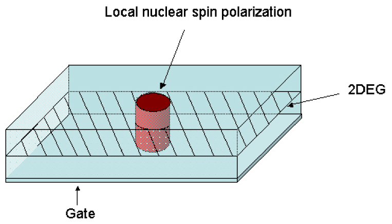
FIG. 1.: The geometry of the proposed experiment: the NSPIQD is created in the region of intersection of the 2DEG with the local nuclear spin polarization.

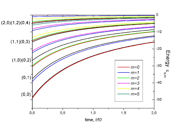
FIG. 2.: Energy spectra of electrons in NSPIQD with initial half-width $d=1\mu$m and $B_{hf}(r=0,t=0)=2.65$T as a function of time in the diffusion regime, $T_{1}/t_{0}=100$. The black lines are the energy levels for parabolic potential labeled by quantum numbers $(n,m)$ at the left. The other lines correspond to the energy levels for the Gaussian potential, the lines having a same color have the same quantum number $m$; the quantum number $n$ is equal to $0$ for the lowest line of each color and increases by $1$ for lines of the same color from bottom to top.

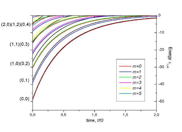
FIG. 3.: Energy spectra of electrons in NSPIQD as a function of time in the intermediate regime, $T_{1}/t_{0}=1$. The parameters of calculations and labeling of levels are as on Fig. 2.

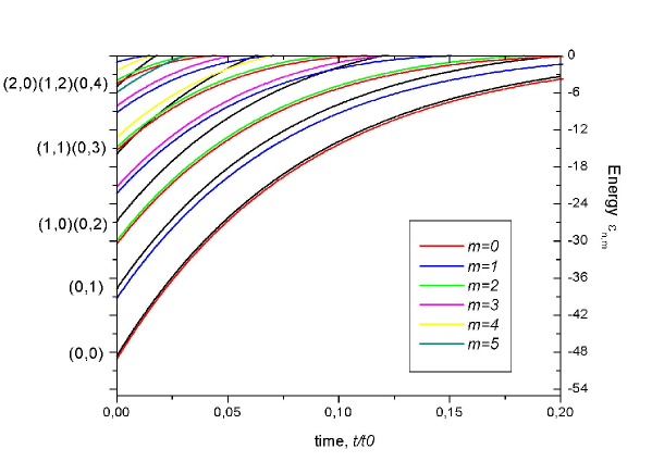
FIG. 4.: Energy spectra of electrons in NSPIQD as a function of time in the relaxation regime, $T_{1}/t_{0}=0.1$. The parameters of calculation and labeling of levels are as on Fig. 2.

REFERENCES

- [1] Quantum Dots, edited by L. Jacak, P. Hawrylak, and A. Wojs (Springer-Verlag, Berlin, 1998).
- [2] M. A. McCord and D. D. Awschalom, Appl. Phys. Lett. 57, 2153 (1990).
- [3] M. L. Leadbeater, S. J. Allen, Jr., F. DeRosa, J. P. Harbison, T. Sands, R. Ramesh, L. T. Florez, and V. G. Keramidas, J. Appl. Phys. 69, 4689 (1991); ]; K. M. Krishnan, Appl. Phys. Lett. 61, 2365 (1992).
- [4] S. J. Bending, K. von Klitzing, and K. Ploog, Phys. Rev. Lett. 65, 1060 (1990).
- [5] M. L. Leadbeater, C. L. Foden, T. M. Burke, J. H. Burroughes, M. P. Grimshaw, D. A. Ritchie, L. L. Wang, and M. Pepper, J. Phys. Condens. Matter 7, L307 (1995).
- [6] F. M. Peeters and A. Matulis, Phys. Rev. B 48, 15166 (1993).
- [7] I. S. Ibrahim, V. A. Schweigert, and F. M. Peeters, Phys. Rev. B 56, 7508 (1997).
- [8] J. Reijniers, F. M. Peeters, and A. Matulis, Phys. Rev. B 59, 2817 (1999).
- [9] For a review see F. M. Peeters and J. De Boeck in Handbook of nanostructured materials and nanotechnology, edited by H. S. Nalwa, Vol. 3 (Academic Press, New York, 1999), p. 345.
- [10] L. Solimany and B. Kramer, Solid State Commun. 96, 471 (1995).
- [11] H.-S. Sim, K.-H. Ahn, K. J. Chang, G. Ihm, N. Kim and S. J. Lee, Phys. Rev. Lett. 80, 1501 (1998).
- [12] N. Kim, G. Ihm, H.-S. Sim and K. J. Chang, Phys. Rev. B 60, 8767 (1999).
- [13] N. Kim, G. Ihm, H.-S. Sim and T. W. Kang, Phys. Rev. B 63, 235317 (2001).
- [14] H.-S. Sim, G. Ihm, N. Kim, and K. J. Chang, Phys. Rev. Lett. 87, 146601 (2001).
- [15] V. Fleurov, V. A. Ivanov, F. M. Peeters, and I. D. Vagner, Physica E 14, 361 (2002).
- [16] Yu. V. Pershin, S. N. Shevchenko, I. D. Vagner, and P. Wyder, Phys. Rev. B 66, 035303 (2002).
- [17] A. Overhauser, Phys. Rev., 92, 411 (1953).
- [18] D. Paget, G. Lampel, B. Sapoval, and V. I. Safarov, Phys. Rev. B 15, 5780 (1977).
- [19] G. Salis, D. D. Awschalom, Y. Ohno and H. Ohno, Phys. Rev. B 64, 195304 (2001)
- [20] D. C. Dixon, K. R. Wald, P. L. McEuen, and M. R. Melloch, Phys. Rev. B 56, 4743 (1997).
- [21] K. R. Wald, L. P. Kouwenhoven, P. L. McEuen, N. C. van der Vaart, and C. T. Foxon, Phys. Rev. Lett. 73, 1011 (1994).
- [22] G. Lampel, Phys. Rev. Lett. 20, 491 (1968).
- [23] Optical Orientation edited by F. Meier and B. P. Zakharchenya (Elsevier, Amsterdam, 1984).
- [24] S. E. Barrett, R. Tycko, L. N. Pfeiffer, and K. W. West, Phys. Rev. Lett. 72, 1368 (1994). For a review see R. Tycko et al., Science 268, 1460 (1995).
- [25] B. E. Kane, L. N. Pfeiffer, and K. W. West, Phys. Rev. B 46, 7264 (1992).
- [26] J. Adamowski, M. Sobkowicz, B. Szafran, and S. Bednarek, Phys. Rev. B 62, 4234 (2000).
- [27] N. Bessis, G. Bessis, and B. Joulakian, J. Phys. A 15, 3679 (1982).
- [28] C.S. Lai, J. Phys. A 16, L181 (1983).
- [29] R.E. Crandall, J. Phys. A 16, L395 (1983).
- [30] M. Cohen, J. Phys. A 17, L101 (1984).
- [31] D. Wolf, Spin-Temperature and Nuclear-Spin Relaxation in Matter (Clarendon press, Oxford, 1979).
- [32] C. P. Slichter, Principles of Magnetic Resonance (Springer-Verlag, Berlin, 1991), 2nd ed.
- [33] D. Paget, Phys. Rev. B 25, 4444 (1982).
- [34] A. Malinovsky, M.A. Brand, and R. T. Harley, Physica E 10 13 (2001).